Preprint
Article

Forecasts of Extreme Meteorological Events Based on Remote Sensed Data Using Machine Learning and Their Effects on Agricultural Productivity

Altmetrics

Downloads

85

Views

39

Comments

0

Submitted:

11 June 2024

Posted:

12 June 2024

You are already at the latest version

Alerts
Abstract
Climate change poses new challenges for agricultural production as an increase in temperature also brings an increase in frequency and intensity of droughts. We study the occurrences of droughts in recent years as well as their effect on agricultural yields in combination with other factors such as winter frost. Furthermore we run experiments that aim to predict future drought events in order to provide insights whether current agricultural products will remain viable long-term and to indicate short-term drought risks. Our study area consists of the South-Moravian region in the Czech Republic and Saxony in Germany with the timeframe ranging from 1990 2022. For the effect on agricultural yields we use statistical methods such as regression and correlation. We train a Long-Short Term Memory (LSTM) neural net on data for the Standardised Precipitation-Evapotranspiration Index (SPEI) in order to predict future events. Our results indicate that the increased severity of droughts in recent years didn’t yet cause yield losses in our researched area. Our predictions with the LSTM look promising, but will need more data for future use-cases in order to increase accuracy and robustness.
Keywords: 
Subject: Environmental and Earth Sciences  -   Remote Sensing

1. Introduction

The impacts of climate change pose major challenges for farmers in growing and cultivating rainfed crops. These include, for example, rising temperatures, more frequent and more severe droughts as well as warmer winters. This means that some agricultural products may no longer be suitable to grow in certain areas, while others may become viable alternatives. For long-term planning, it is then essential to accurately predict future trends in climate change and drought events.
This work has several contributions. First, we study the impact of various climate-dependant factors on agricultural productivity. We identify drought, spring frost and growing degree days (GDD) as the most relevant factors affecting crop yields. Regression and correlation methods are employed to quantify their effect. The second goal is to predict future drought events by training a Long-Short Term Memory (LSTM) [1] neural network on the Standardised Precipitation-Evapotranspiration Index (SPEI) [2] data. Finally, and of a more secondary character, we aim to gain an understanding of local differences in climate on a small scale. To achieve this goal, we compare the models that we use to measure the effects of climatic factors on crop yields with respect to the size of the input regions.

1.1. Weather Forecasting with Machine Learning

Rhee and Im [3] employed various tree algorithms, such as Decision Trees, Random Forest, and Extremely Randomized Trees, to predict SPI and SPEI using remote sensed data. They applied these algorithms to an area in South Korea which consists mostly of forests and to a lesser degree agriculture, as well as urban areas. Their experiments showed that the Extremely Randomized Trees model performs best with a yielded accuracy of 56% for SPI and 64% for SPEI. The authors acknowledged the possibility of further improvement and suggested utilizing these findings as a benchmark for future research. Sobia Wassan and Binte-Imran [4] utilized a Convolutional Neural Network (CNN) for forecasting frost events. They predicted surface temperatures based on soil temperatures with a 98.6% accuracy using virtual data from the United States. The source of virtual data is unspecified, while the remaining data was obtained from weather stations in the United States, with test data accounting for 20% and training data accounting for 80%. Weyn et al. [5] used a “Deep Learning Weather Prediction” (DLWP) model to predict 6 different atmospheric variables 2 6 weeks ahead. They compared their results with those of the European Centre for Medium Range Weather Forecasts (ECMWF) [6]. For short-term forecasts of 2 3 weeks, the aforementioned numerical models still held a clear superiority. However, for extended durations, the DLWP was nearly on par.
Recently, the prediction of SPEI using LSTM has also been the subject of research. Dikshit et al. [7] described an LSTM model with drought data from Australia for the period 1901 2018 , achieving R 2 correlation coefficient of 0.998 for the training data and 0.996 for the validation data, and a Mean Average Error (MAE) of 0.012 and 0.01 respectively.

1.2. Influence of Drought and Frost on Yields

Jamieson et al. [8] investigated the impact of drought on barley, wheat, and corn by implementing experimental methods of selectively irrigating plants. They identified varying effects of drought dependent on the plant’s growth stage during the event. Barley experiences reduced grain number and size, when exposed to drought in its early growth stage, whereas later exposure results in lower grain number and sieve loss. Kolář et al. [9] examined the influence of climatic conditions on low yields of spring barley and winter wheat in the Southern Moravian Region between 1961 and 2007. They concluded that various factors contribute to low yields, including high temperatures and droughts in spring as well as unfavorable conditions during winter. Mansoor Maitah and Maitah [10] analysed how rainfall and temperatures affect maize production in the Czech Republic between 2002 and 2019. They aimed to identify reasons behind the decline in maize production since 2010. They identified the months of July and August as the critical period when poor conditions cause the most damage. Labudová et al. [11] compared the relationships and impact of SPI and SPEI on crop production ( 1996 2013 ) in certain parts of Slovakia. The study found that, despite some regions displaying no significant correlation between crop yields and droughts, SPEI indices were, for the most parts, more informative than SPI. In particular, SPEI with scale 3 performed best.
Zheng et al. [12] conducted an analysis of frost trends and their effects on wheat yields in Australia. Their findings indicate that rising temperatures associated with climate change have an adverse impact on frost, leading to an increased likelihood of critical post-head-emergence Frost (PHEF) due to the earlier arrival of the post-head phase. Additionally, the last frost day occurs later on average. The development of frost-resistant wheat varieties is recommended. Frederiks et al. [13] stated that this has been a long-standing area of current research, but the attempts have been largely unsuccessful thus far.
Kukal and Irmak [14] examined the interaction of various temperature-dependent parameters on crop yields between 1900 and 2014, including Growing Degree Days (GDD), duration of the growing season, and frost. They showed that, on average, per century, the first fall frost has been occurring later by 5.4 days, and the last spring frost has been occurring earlier by 6.9 days, which means an average lengthening of the growing season by 12.3. Annual GDD has increased by a total of 50°. The prolonged frost-free period has a positive effect on yield, while the increased GDD has a slightly negative effect. The R 2 coefficients derived from the regression analysis of the harvest and GDD are ranging from 0.07 to 0.34, making the assertions partly ambiguous. Wypych et al. [15] analysed the impact of climate change on GDD in Poland between 1950 and 2010, and found a noticeable increase. While the rise in GDD might lead to positive effects on crop yields, there is also a potential risk of frost-related losses if the last frost occurs after plant growth has already commenced in spring. Trnka et al. [16] studied agro-climatic conditions in Europe in the context of climate change in the period 1970 2000 with an outlook to 2050. They expected the risk of climate-induced crop failure to increase, making it advisable to diversify agricultural production in order not to be dependent on single vulnerable products. The most relevant publication for our research is the work by Potopová et al. [17]. They studied the impact of drought on crop yields in the South Moravian Region between 1961 and 2012, using SPEI indices. Results indicated that there was a correlation between crop yields and droughts during certain months, ranging from 0.31 (grapes) to 0.6 (cereals).

2. Study Area and Datasets

2.1. Study Area

The study focuses on two regions: the South-Moravian region in the Czech Republic and Saxony in Germany. The South-Moravian region is located in the south-eastern part of the Czech Republic, between 48 37 N and 49 36 N latitudes and between 15 32 E and 17 38 E longitudes. It borders with five Regions of the Czech Republic as well as with Austria and Slovakia. The Region covers an area of 7196.5 k m 2 with a minimum elevation of 150 m and maximum elevation of 842 m . 60% of the region is agricultural land, 83% of which is arable. Agriculture in this region focuses on cereals, rapeseed, as well as grain and silage maize. Additionally, the South-Moravian Region is the center of viticulture in the Czech Republic – 90% of the vineyards of the country are located in this Region [18].
Saxony is the easternmost federal state of Germany. It lies between 50 10 N and 51 40 N latitudes and between 11 52 E and 15 2 E longitudes and borders with the Czech Republic and with Poland. Saxony covers an area of 18450 k m 2 with a minimum elevation of 40 m and maximum elevation of 1235 m . The majority of Saxony is flat land, while the southern border is mostly mountainous. 54% of the area is used for agriculture focusing on cereals, root crops - potatoes and sugar beet, rape seed, and forage plants - grain and silage maize [19]. The climate in both regions is temperate, which is typical for central-European countries. Saxony is located Northwest of South-Moravia, with a significant geographical distance between the two regions.

2.2. Datasets

The used sets for weather data were provided by meteoblue [20]. Their API allows to download historical datasets with varying sources. For this work a dataset called Nems4 is used which is modeled by meteoblue and ranges back to the year 2008. Older data is filled using ERA5, the reanalysis dataset of the ECMWF [6]. For our purposes, we downloaded monthly precipitation and potential evapotranspiration, as well as daily minimum and maximum temperatures 2m above ground. With this data, we compute the SPEI, frostdays and GDDs. This is further described in Section 3.3 In the South Moravian Region, values are missing between April and June for the year 2004. Therefore, no SPEI could be computed for those months. The Saxon data is complete. This results in 448, respectively 168 distinct sets of timeseries for Saxony and South-Moravia. For testing purposes of the LSTMs, we also downloaded precipitation and evapotranspiration data beginning east of Saxony and reaching several hundred km eastwards. This data is split into 2 separate sets and will be used to calculate results, shown in Section 4.
The data for crop yields for the South Moravian Region stems from it’s statistical yearbook [18]. Data from this region was used between 2002 and 2019. Earlier yield data was recorded in a different way and is therefore not published. Saxon data is published by the “Statistisches Landesamt Sachsen” [21] and available from 1990-2021. Both datasets contain yearly crop yields in tonnes per hectare [t/ha] for the entire recorded areas. After excluding incomplete timeseries, we are left with Saxon data for wheat, winter wheat, rye, winter barley, spring barley, oat, triticale, grain maize, silage maize, potatoes, sugar beet, rape and grain. The South-Moravian data includes wheat, barley, potatoes, sugar beet, rape and vine.

3. Materials and Methods

3.1. Drought Index SPEI

Drought describes a long, dry period. It is a major factor with regards to harms on vegetation and crop yields. To quantify droughts, several indices were developed [22]. For this work we compute the Standardised Precipitation-Evapotranspiration Index (SPEI), as it is recommended by several sources we presented in Section 1.1 and as the necessary data is available. The SPEI is an extension of the previously and currently used Standardised Precipitation Index (SPI) [23], which scales precipitation over a long period of time, to calculate the duration and intensity of droughts that occurred within an observed time frame. The SPEI was presented in 2010 by Vicente-Serrano et al [2]. The idea behind it is to combine the advantages of the SPI and PDSI (Palmer Drought Severity Index [24]), while negating their disadvantages. It is a multi-scalar index that uses precipitation and evapotranspiration as input in order to calculate the beginning, duration and intensity of drought periods.
The SPEI calculates the difference (D) between precipitation (Prec) and potential evapotranspiration (PET) D i = P r e c i P E T i for all months i in the dataset, before standardising and scaling D. Due to the full calculation being too extensive for this paper, we refer to [2] for the detailed description. The resulting index values range from 3.0 , which describes an extreme drought, to 3.0 which describes an extremely wet period. For each time series with values for precipitation and evaportranspiration a calibration period is selected. Data from the calibration period will be used to set the scaling parameters for the whole time series. The mean of the SPEI during the calibration period is 0 and the variance 1.
Table 1. Classification of SPEI-values
SPEI Classification
> 2.00 extremely wet
( 1.50 , 2.00 ] severely wet
( 1.00 , 1.50 ] moderately wet
( 1.00 , 1.00 ] nearly normal
( 1.50 , 1.00 ] moderately dry
( 2.00 , 1.50 ] severely dry
2 extremely dry
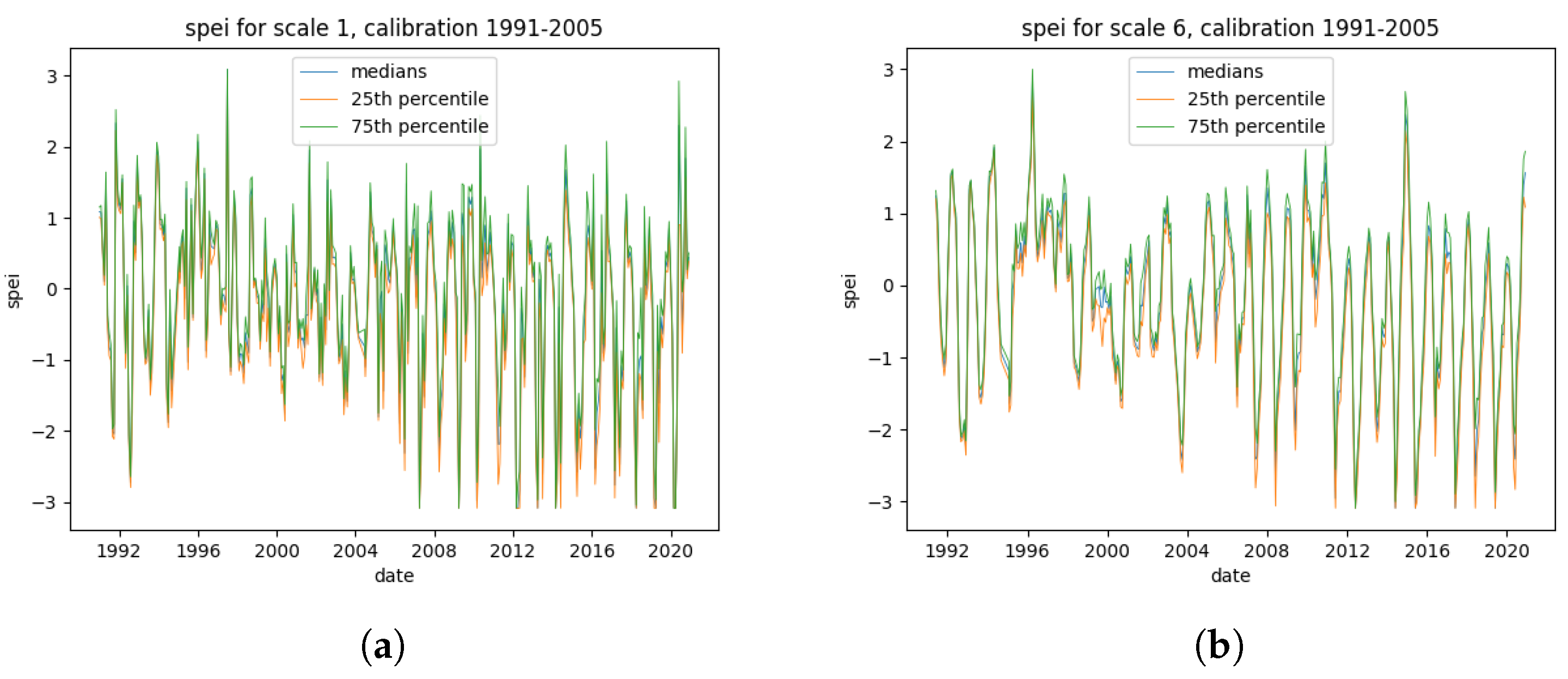
The SPEI is computed on the data provided by meteoblue with the Python package "climate_indices" [25]. A variety of calibration periods were tested. In this work we used calibration periods ranging from 1990 2005 unless specified otherwise. Table 2 gives an overview for the SPEI values for Saxony for the different scales. As can be seen, the mean values are negative, which means the time not included in the calibration period was generally more dry. Furthermore, the occurrence of long droughts has increased as the SPEI 6 value is the lowest. A visual representation is given in Figure 1 in which the South-Moravian SPEI time series are shown. These plots also indicate a strong increase in frequency and severity of droughts in recent years. Additionally, they serve to illustrate that time series of an SPEI with a higher scale are much smoother compared to the SPEI 1. This also makes the prediction much easier which will be shown and discussed in Section 4 and Section 5.

3.2. LSTM

An artificial neural network (ANN) is a type of machine learning model inspired by the function and structure of the human brain. ANNs consist of interconnected nodes – artificial neurons – organized in layers, which process information, learn from it and transmit it. ANNs can be trained to perform various tasks such as classification and pattern recognition. Recurrent Neural Networks (RNNs) are a specific type of ANNs that can process sequential data by using feedback connections, allowing information to persist from one step to the next. Long Short-Term Memory (LSTM) [1] is a variant of RNN that addresses the vanishing gradient problem, which can occur when training traditional RNNs. LSTMs employ memory cells and gating mechanisms that can store information over longer periods of time and selectively retain or forget information based on the input data. These mechanisms make LSTMs effective at capturing long-term dependencies in sequential data and have been successfully applied in various fields such as language processing and time series analysis [26,27].
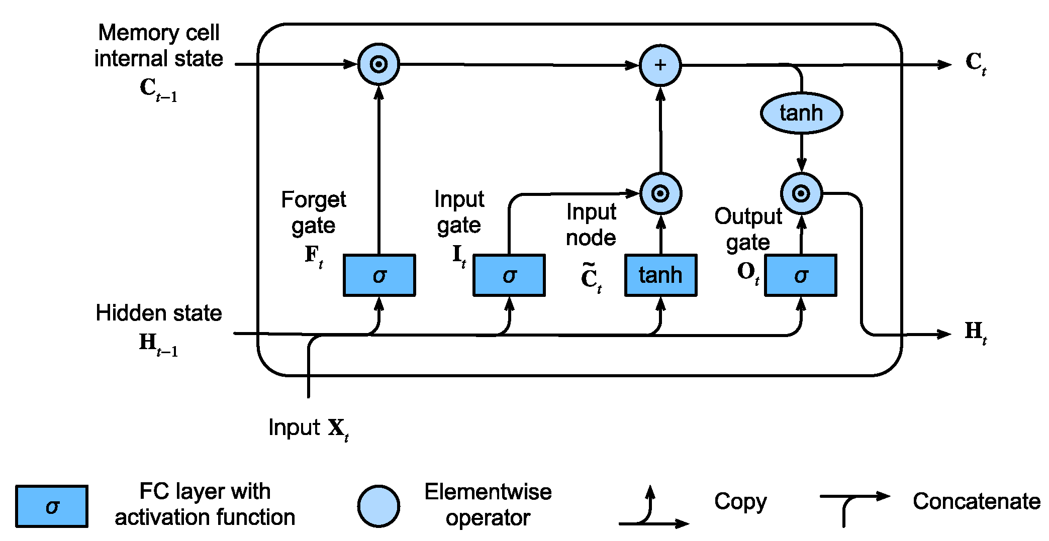
Figure 2 depicts the architecture of an LSTM unit. At time step t, the unit uses the input sequence X t , the hidden state H t 1 and the memory cell internal state - which serves as the long-term memory C t 1 , both from the previous time step, to update the hidden state H t and memory cell internal state C t . The LSTM unit has three gates to control the flow of information by employing activation functions. The sigmoid activation function σ ( x ) = 1 1 + e x transforms values to the range [ 0 , 1 ] ; this helps to update data or forget it, a value of 0 means that the component is irrelevant and should be forgotten and a value of 1 indicates that the component is relevant and shall be retained. The hyperbolic tangent function t a n h ( x ) = 1 2 e 2 x 1 transforms values to the range [ 1 , 1 ] as means of regulating the network.
The forget gate  F t controls which information stored in the memory cell to forget.
F t = σ ( W x f X t + W h f H t 1 + b f )
The input node (or cell candidate state) C t ˜ , provides a proposal for new values that could be added to the cell state.
C t ˜ = tanh ( W x c X t + W h c H t 1 + b c )
The input gate  I t governs which new information provided by C t ˜ will be encoded into the cell state.
I t = σ ( W x i X t + W h i H t 1 + b i )
Next, the cell state at time t, C t is computed by employing I t to determine how much information to use via C t ˜ and by employing F t to determine how much information to retain from the old cell internal state C t 1 , where ⊙ is the Hadamard product operadwdtor, i.e., elementwise multiplication of of vectors.
C t = F t C t 1 + I t C t ˜
The output gate controls which information from the current cell state should used be in the output.
O t = σ ( W x o X t + W h o H t 1 + b o )
Finally, the resulting values C t and O t are utilized to compute the hidden state at time t, H t .
H t = O t t a n h ( C t )
Here W x f , W x c , W x i , and W x o are weight parameters of the current input sequence, W h f , W h c , W h i , and W h o are weights of the previous hidden state and b f , b c , b i , and b o are bias parameters.
The training of the LSTM is done with the Keras framework[28], which is based on Tensorflow [29]. The input data comprises of the SPEI time series. We experiment with different splits for the training and validation data:
  • Split the data by region. Training set has SPEI-values for all dates.
  • Split the data by time with validation data consisting of the most recent years.
  • Split the data by time, using the first available years as validation data.
The reason for different splits for the training and testing data is the proximity of neighboring timeseries. As the data is very similar in many cases, a random split would lead to overfitting. By setting the split manually according to the listed rules, the goal is to decrease the amount of nearly identical timeseries in different parts of the dataset. In the first case all sets contain data spanning the whole temporal range.
The 2nd and 3rd cases contain temporal splits. Theoretically, the 2nd case is more intuitive, as for any given time series as input, the value to predict comes after the input. This is also true for the 3rd case, but in contrast, the timeframe of the test set precedes the timeframe of the training set. This is an experimental setup to test whether the results differ from using the standard order.
For the final test dataset, we obtained SPEI time series for a region located East of Saxony. When training and validating a LSTM in a single region, such as Saxony, a split of approximately 80 : 20 is used. If the validation region is different, such as South Moravia, the full data of the first region is used during the training.
The training process consists of applying LSTM to sequences of consecutive SPEI-values represented as x 0 x n to predict the subsequent SPEI-value represented as y. A training data example is presented in Table 3 where four SPEI-values are used to predict the fifth. Depending on the scale x 0 x 3 consist of SPEI-values for n months, where n = 4 + s c a l e 1 . The table illustrates that each input sequence is the previous input sequence shifted to the left, with the previous output value y being used as the last input x n . To determine the feasible range of input sequence lengths we conducted an experiment comparing LSTMs with sequence lengths varying between 1 and 120 values.
Due to the lack of sufficient training data we employ data augmentation by replicating each training sequence 10 times and adding a Gaussian noise with a mean value of 0 and variance of 0.05 to each element of our input sequences. Additionally, to enhance the robustness of the LSTMs, the added noise is recalculated at each iteration of the training process. Thus, during training, the example presented in Table 3 may transform into the one shown in Table 4.

3.3. Measuring the effect of climatic factors on crop yields

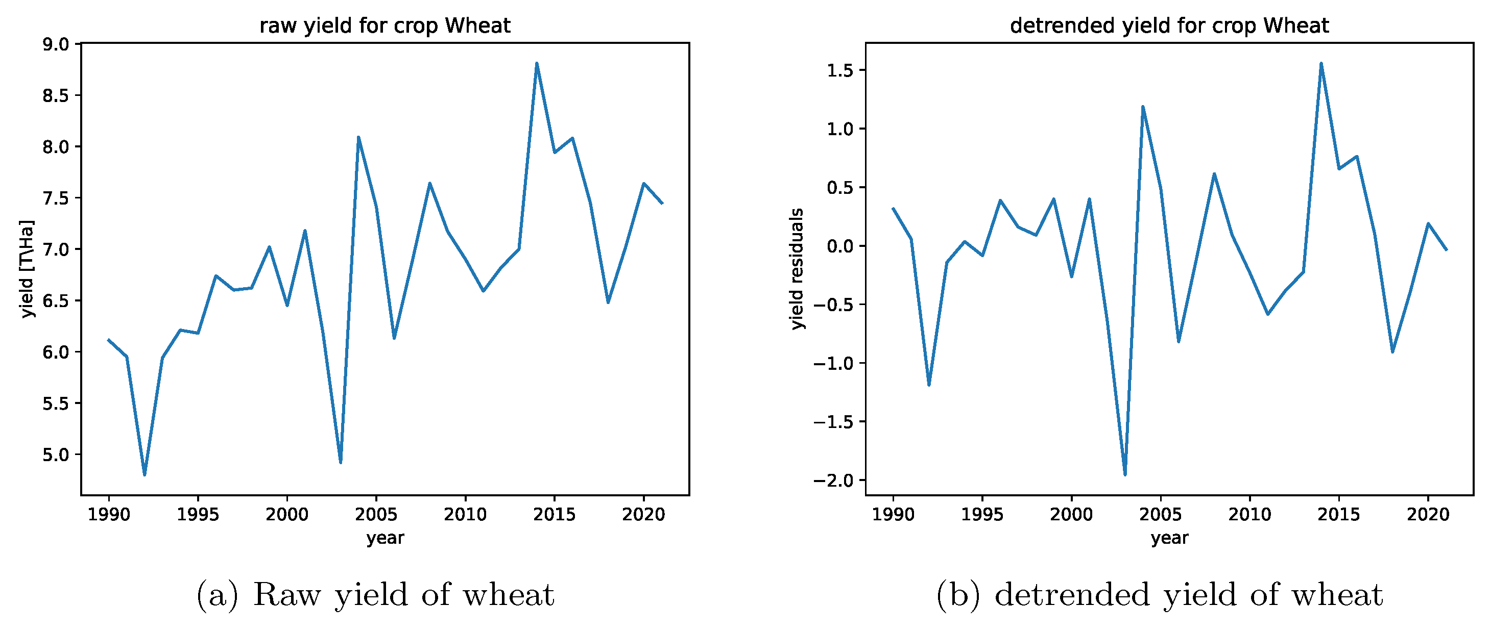
To investigate the impact of extreme meteorological events, such as drought and frost, on crop yields, we used correlation and regression methods. As described in Section 2.2, the crop yield data is available in yearly time series, while the SPEI data is monthly. To ensure that the time series are of equal frequency, we divided the SPEI time series by month, resulting in 12 different annual time series for each SPEI scale. As the tests covered scales 1, 2, 3 and 6, we thus derived 48 time series for each coordinate. The median values were then calculated for each time series set accross all available coordinates. For instance, the SPEI 3 value for April in a given year represents the median of all SPEI values from the entire region. Correlations between the SPEI time series and the available crop yield time series were measured. Several example results are presented in Section 4.2. Correlations were measured on the raw crop data and after applying a two-step detrending method. In the first step, a regression was calculated on the data to find the general trend in yield values. The trend was then subtracted from the yield data. This eliminates the effect of climate change on crop yields, as well as other factors that cause long-term changes in crop growth, such as technological advancements. Following this, standardization is carried out via a z-score transformation (Equation 7)).
Z = X μ σ ,
where X is the crop yield value, E ( X ) = μ is its expected value, and V a r ( X ) = σ 2 is its variance. The transformation has the properties of E ( Z ) = 0 and V a r ( Z ) = 1 . Figure 3 shows a comparison of the raw and detrended yields of wheat in Saxony.
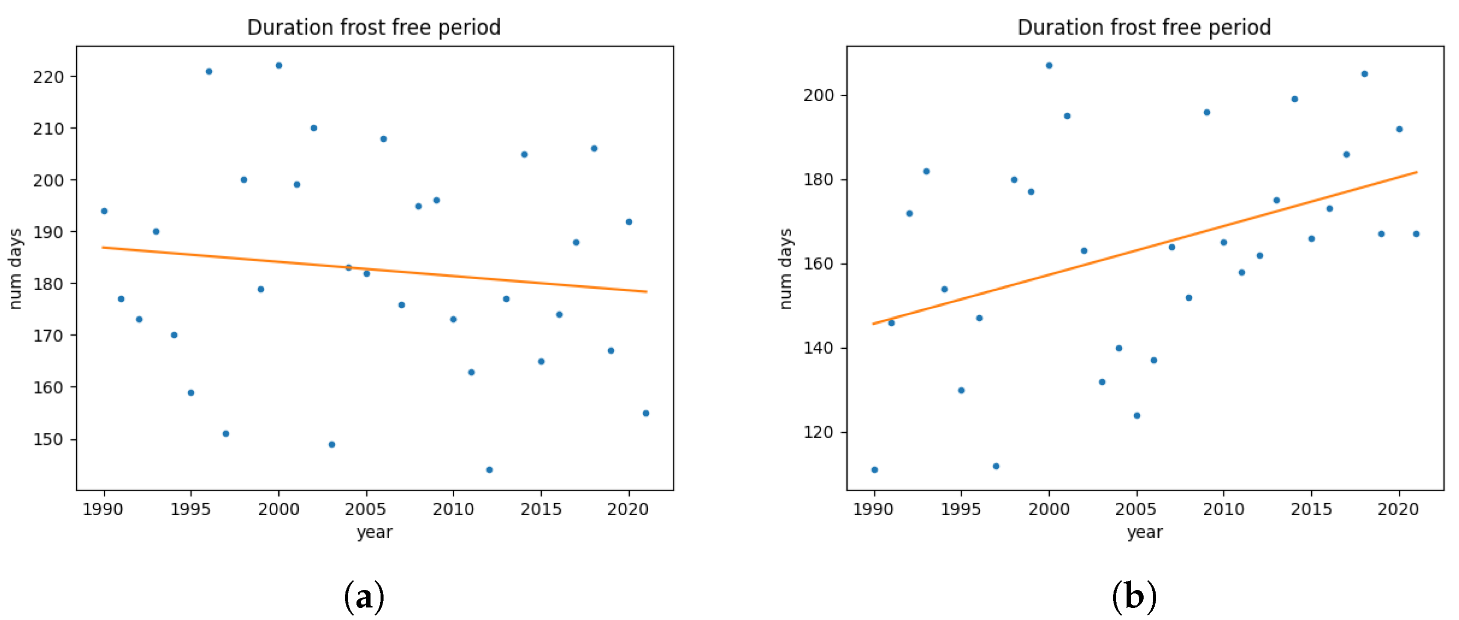
Other climatic factors that can affect plant growth are frost occurrences and Growing Degree Days (GDD) [30]. To examine the influence of frost, we extracted several parameters from the minimum temperatures. This includes the duration of frost-free periods, the occurrence day of the last spring frost and the occurrence day of the first winter frost for each year. No trend was found for the duration of the frost-free period in Saxony, as shown in Figure 4. The figure shows two scatter plots for the annual number of frost-free days with a corresponding regression line for two locations in Saxony. Depending on which location - and therefore distinct time series - is selected, the trend of the frost-free duration points towards a different direction.
The GDD [30] is a heuristic used to estimate the stages of plant growth, phenological phases, by measuring heat units. It is based on the dependence growth stage on the accumulated heat during the growing season. GDD can be calculated on a daily basis using the following formula:
G D D = T m a x + T m i n 2 T b a s e ,
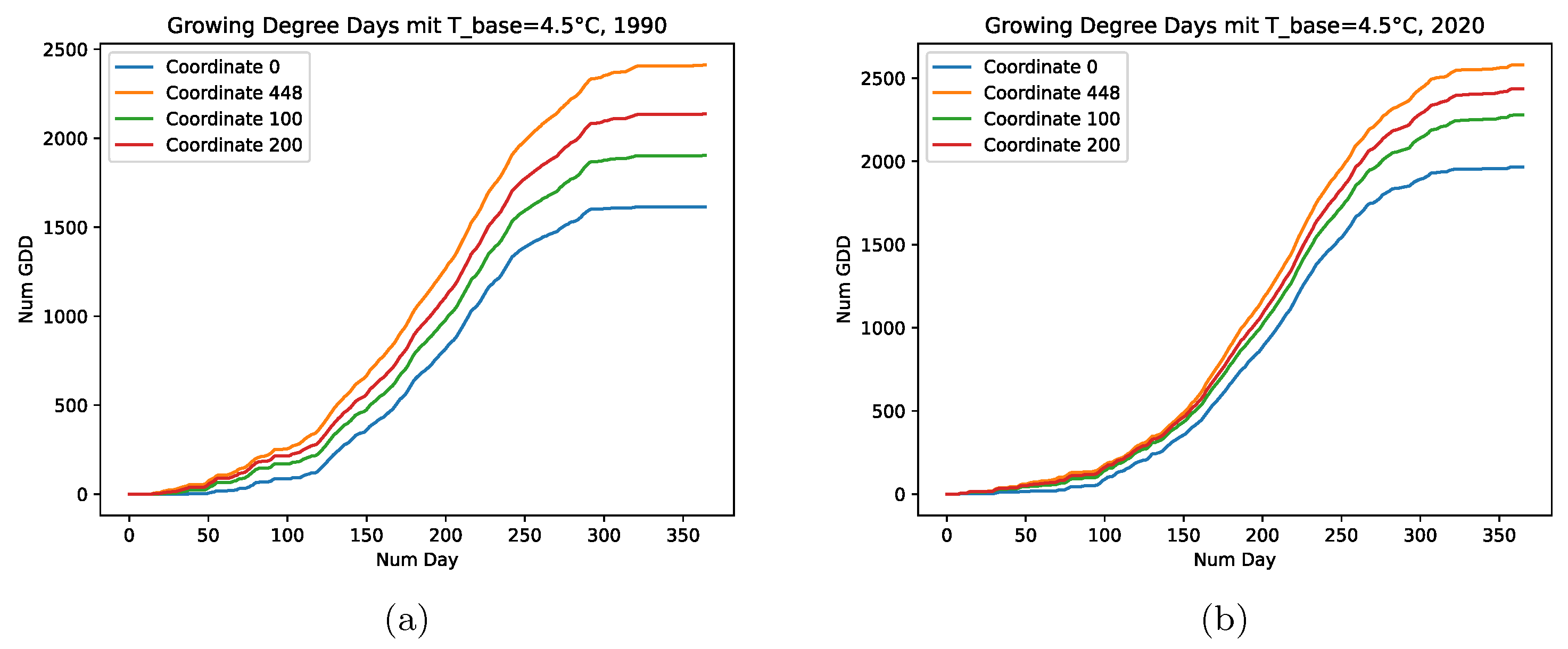
where T m a x and T m i n are the daily maximum and minimum temperatures, respectively, and T b a s e is the base temperature. The base temperature is dependent on the plant and describes the temperature required for plant growth. GDD values are calculated so that they can never fall below 0 (e.g., in the case of T m a x < T b a s e ) and can take values greater than 1 for a given day. This work uses the accumulated GDD (AGGD), which is a time series for a single year with daily values representing the sum of GDD up to that day. Figure 5 shows example plots for AGGD in Saxony given a base temperature of 4 . 5 C for the years 1990 (Figure 5a) and 2020 (Figure 5b). It can be observed that some locations are generally warmer than others, which was also the case for the years in between.
A correlation analysis was conducted between yearly crop yields and any of the time series for frost-free periods, day of last spring frost, or day of first winter frost. The results showed only minor correlations at best. Additionally, there was no significant correlation found between GDDs at certain times and crop yields.
To further investigate the effects of climatic factors on crop yields, we developed a new method that combines the inputs that are insufficient on their own. We measure the synergistic effects of different factors by implementing a second-order polynomial regression to predict crop yields. The metric we use to evaluate the regression is the R 2 score between the measured crop yields and the predictions. Due to the limited size of the data, the analysis was conducted on the full dataset without removing any entries for testing purposes. The feature size was restricted to three. After testing a variety of configurations, the resulting regression model includes values for the monthly SPEI, the number of days since the last spring frost, and the accumulated GDD at the time of the last spring frost. Other configurations may achieve similar or partially better results. The aim of this approach is not to attain the highest possible score, as this method is prone to overfitting and generating false positives. Therefore, the described features are used as the final configuration for this study. The results of this experiment are presented in Section 4.2
4. Results

4.1. LSTM

Due to results during the experimental stage, Adam was chosen as optimizer, ReLu as activation function and MSE as loss function. We added a dropout layer with a value of 0.2 . The layer sizes are 16 for the hidden layers and 4 for the fully connected layer. The LSTMs are trained for 1000 epochs with early stopping.
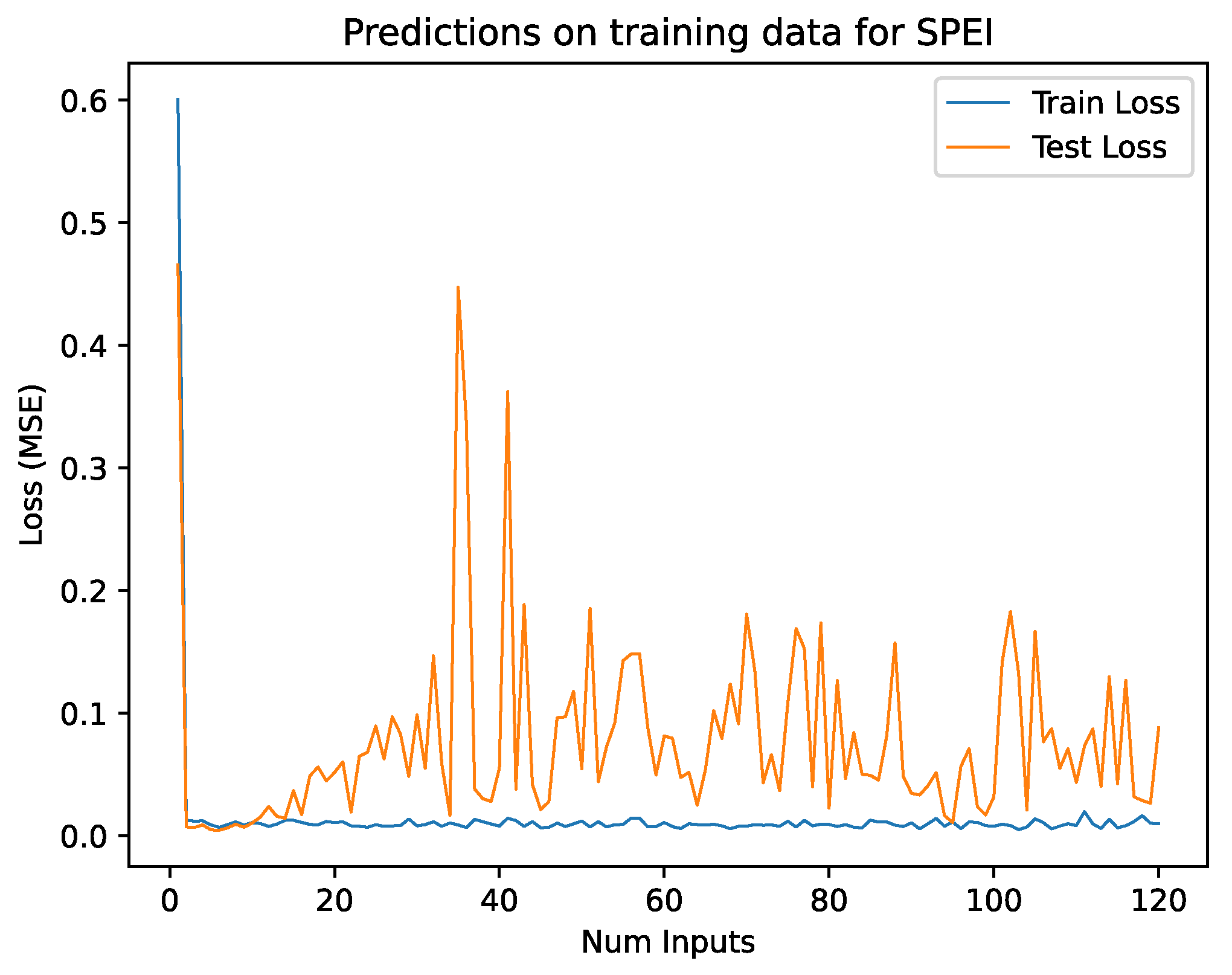
The length of input sequences is determined via an experiment in which sequence lengths between 1 and 120 values are tested. Figure 6 shows train- and test losses for a continuum of varying input lengths. For this trial the SPEI 3 dataset from South-Moravia serves as training data and the dataset from Saxony as test data.
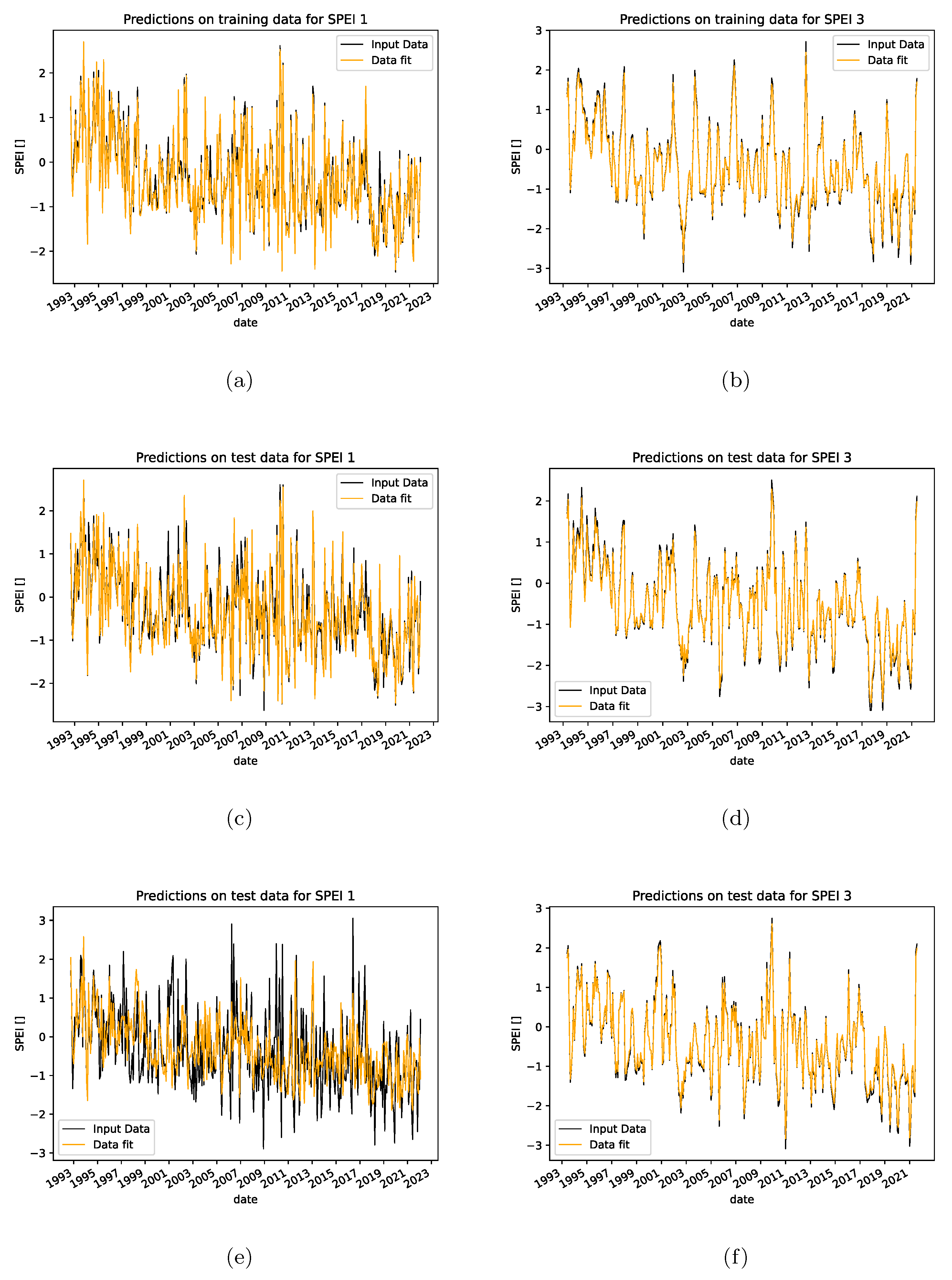
Figure 7 shows a comparison of a LSTM trained with SPEI 1, shown in the left column and a LSTM trained with SPEI 3 shown in the right column. The LSTMs are trained with a subset of the Saxon data and validated with the remaining data from Saxony. The plots show the ground truth data - the calculated SPEIs - of a single timeseries in black and the predicted SPEIs of the same timeseries in orange. The first row shows the input data and data fit for the training data. In this case both predicted series have a high accuracy as expected. The 2nd row shows the input data and data fit for the validation data. Here, the quality of the fit remains the same for the SPEI 3-LSTM, while the fit of the SPEI 1-LSTM shows a higher deviation from the ground truth. This trend continues for the test data which is shown in row 3. The scale 3 fit is still very accurate while the scale 1 fit produces substantial errors.
We present a general overview for the resulting metrics of the LSTMs in Table 5 and Table 6. The training data is a subset of the Saxon dataset. The columns “Loss Test 1” and “Loss Test 2” show test losses for regions east of Saxony, which were described in Section 2. These test sets contain the full data for the respective region. The plots in Figure 7 are described in the first 2 rows in Table 5. The LSTM using SPEI 1-data has a low training loss and an only slightly higher test loss for the remaining Saxon data. It lacks robustness to spatial differences, as the test losses for the regions that are further away are much higher. The SPEI 3-LSTM shows no lack of accuracy on the test data. Rows 3 and 4 describe LSTMs with a temporal split of training and test data. The test data consists of the last 5 years recorded for the whole region of Saxony. The overall results are much worse for the scale-1 LSTM, with a similar quality for scale-3. When the order of the training and test sets is reversed, as in rows 5 and 6, the LSTM with SPEI 3 also has problems with accurate predictions. Especially the predictions for the Saxon test data yield a high loss. The predictions for the 2 test regions are very accurate, but slightly worse compared to the other LSTMs with SPEI 3.
Table 6 shows the variances of the ground truth data and the predictions of the LSTMs. We recorded this data, because first experiments always resulted in LSTMs with very low variances on forecasts. As can be seen, the variance for the SPEI 1-LSTMs are in the same range on the training data, but decrease drastically on the test data. With regards to scale 3, the variance is always slightly lower on the test data. This concurs with the visual representation in Figure 7, where the peaks of the ground truth data are always higher than the data fit. In case of the inverted temporal split of the training/test data, the variance is also much lower on the Saxon test data. In general, this shows that, if the data cannot be predicted by the LSTM, the LSTM will predict a value close to 0.
In order to evaluate how far into the future a resulting LSTM can give accurate predictions, we run an experiment where only a single input is fed into the trained LSTM. Within each step, the LSTM makes a prediction, which is then inserted at the end of the next input sequence. As the length of the input sequence is 48, after 48 steps the inputs solely consist of predicted values. The predictions are very accurate in the beginning, with a precision comparably to Figure 7c. After some years, there are several occurrences in which the LSTM fails to make an accurate prediction. However, those inaccurate predictions only have a negligible impact on the following forecast.

4.2. Correlation between climate indicators and crop yields

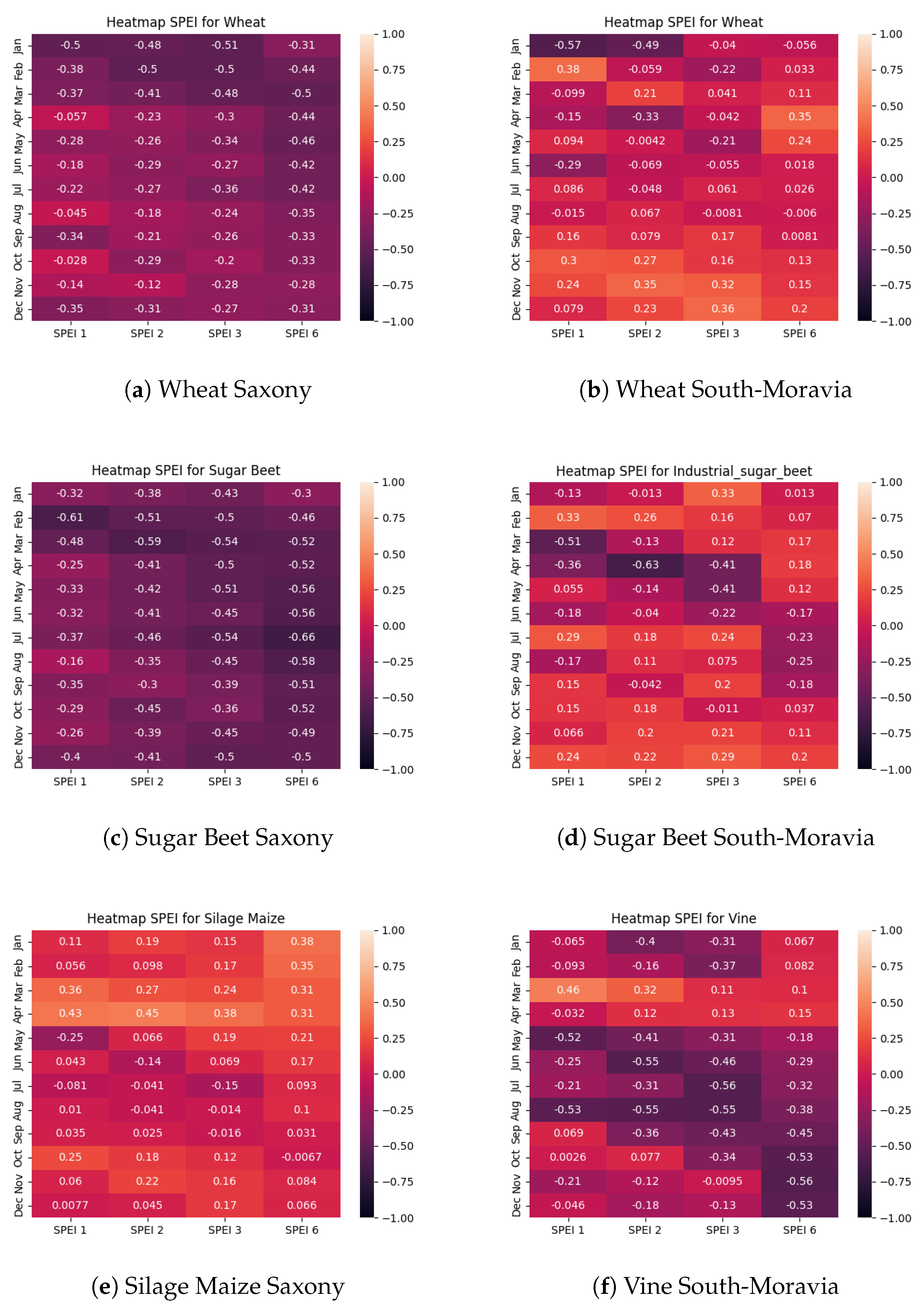
Figure 8 contains several heatmaps that show the correlation between SPEI and crop yield of wheat, sugar beet and silage maize in Saxony (Figure 8a,c,e), as well as wheat, sugar beet and vine in South Moravia (Figure 8b,d,f). While the heatmaps for silage maize and vine are not comparable, those results are included because of the significance of vine production to the South-Moravian Region and because silage maize is the only Saxon crop with some positive correlation between SPEI and yearly yields.
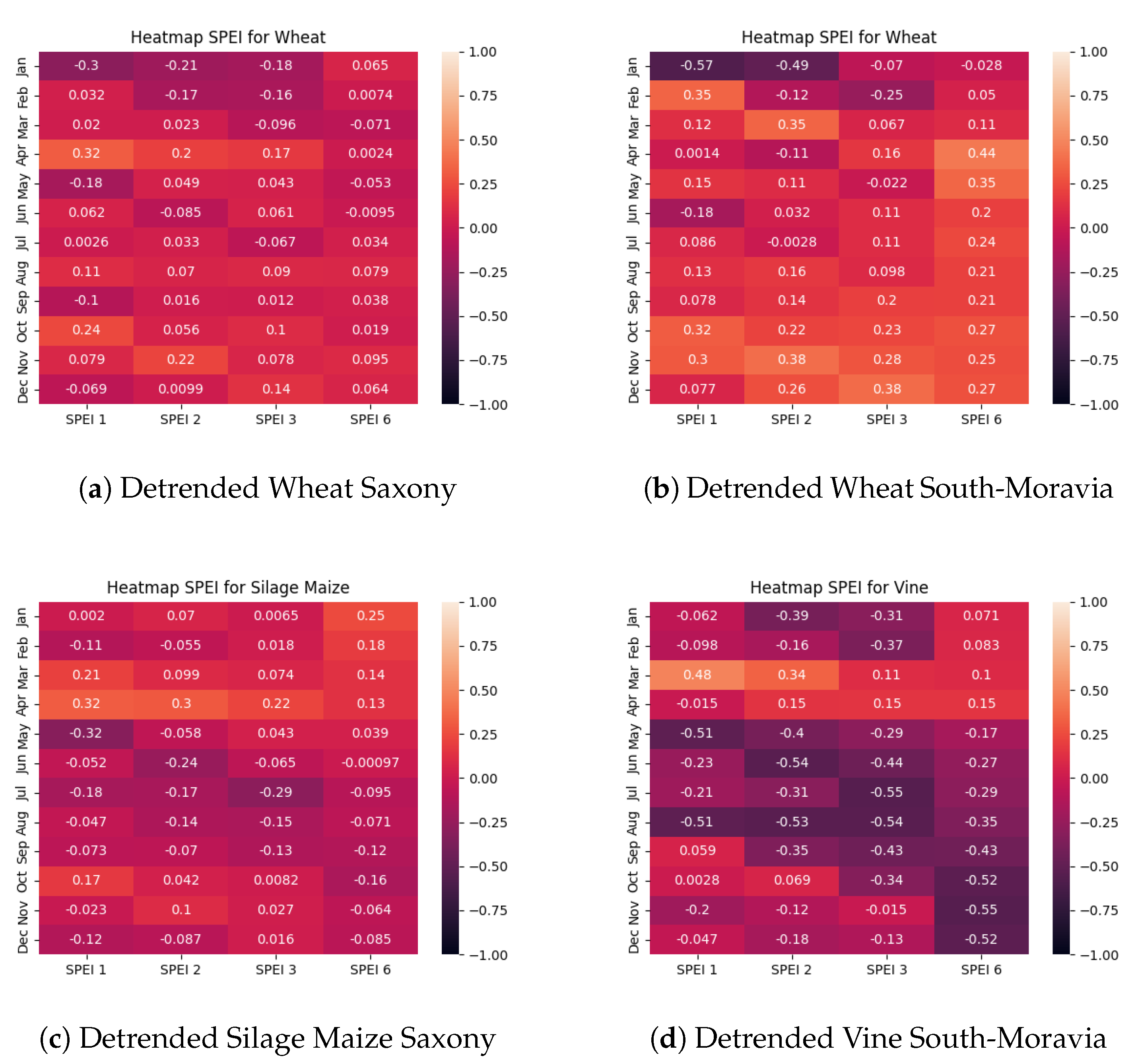
The most surprising result for Saxony is that crop yields show a negative correlation to SPEI. This indicates that crop yields were better in generally drier years. When looking at the raw data, two aspects are visible: There has been an increase in frequency and severity of droughts as well as an increase in crop yields. Regarding the reunification of Germany in 1989, it is likely that a major factor of the increase in crop yields is technological advancement. Figure 9 shows the correlations between SPEI and detrended crop yields for the same crops as in Figure 8. Sugar beet is not included, because it doesn’t add any additional insight. As can be seen in Figure 9a, almost all correlations for detrended wheat yields in Saxony are close to 0. The highest absolute values are 0.3 in January and 0.32 in April, both for SPEI 1. Those results are meaningless, as SPEI 1 is most susceptible to noise. With regards to detrended wheat yields in South-Moravia, the results are slightly different, as the SPEI 6 shows some correlation in April and May and a very weak correlation after. As the SPEI 6 includes 6 months, the value for April includes droughts until the end of September.
Table 7 displays the available crops for Saxony along with R 2 -values achieved when applying a polynomial regression of second order between yearly crop yields and a combination of SPEI 3/6-values, which are split by month, occurrence dates of the last yearly spring frost, and GDD at the date of the last spring frost. To calculate the date of the last spring frost we decided to make the threshold temperature a variable, as R 2 -values show significant improvements in quality with adapted thresholds. For Saxony, in order to not have any missing data, the lowest possible frost temperature is 7 C , but as is shown in the result table, the lowest used temperature is 5 C . We assume this approach is viable, because generally, if R 2 -values are the highest at e.g. 4 C , the scores are higher for 3 C than for 2 C . This effect diminishes though for temperatures further away.
As a polynomial regression with 3 features includes many degrees of freedom, a certain level of R 2 -values will always be achieved. During the whole experiment, R 2 -values rarely fell below 0.2 . Therefore we conclude, that this method shows no significant results for triticale and rye. We discuss possible reasons for this finding in Section 5. For most investigated crops, the relevant months are between February and April. When comparing these results with those visualized in Figure 8, there is a significant overlap with the most relevant months for correlations. This statement cannot be made for sugar beet, because the correlations between SPEI and crop yields are similar throughout all months. The results are most surprising for silage maize, as the correlations are lowest from August-October, which is when the R 2 -values from the regression are highest.
We have not include results for regressions made with detrended crops, because the value ranges of the values are similar. There were only some differences with regards to the most significant months. For the South-Moravian Region, the regressions can also be calculated, but as the crop timeseries contains less than 20 entries, we assume the feature space of this methodology is too large in order to produce operable results.

4.3. Scalability of Regression Models

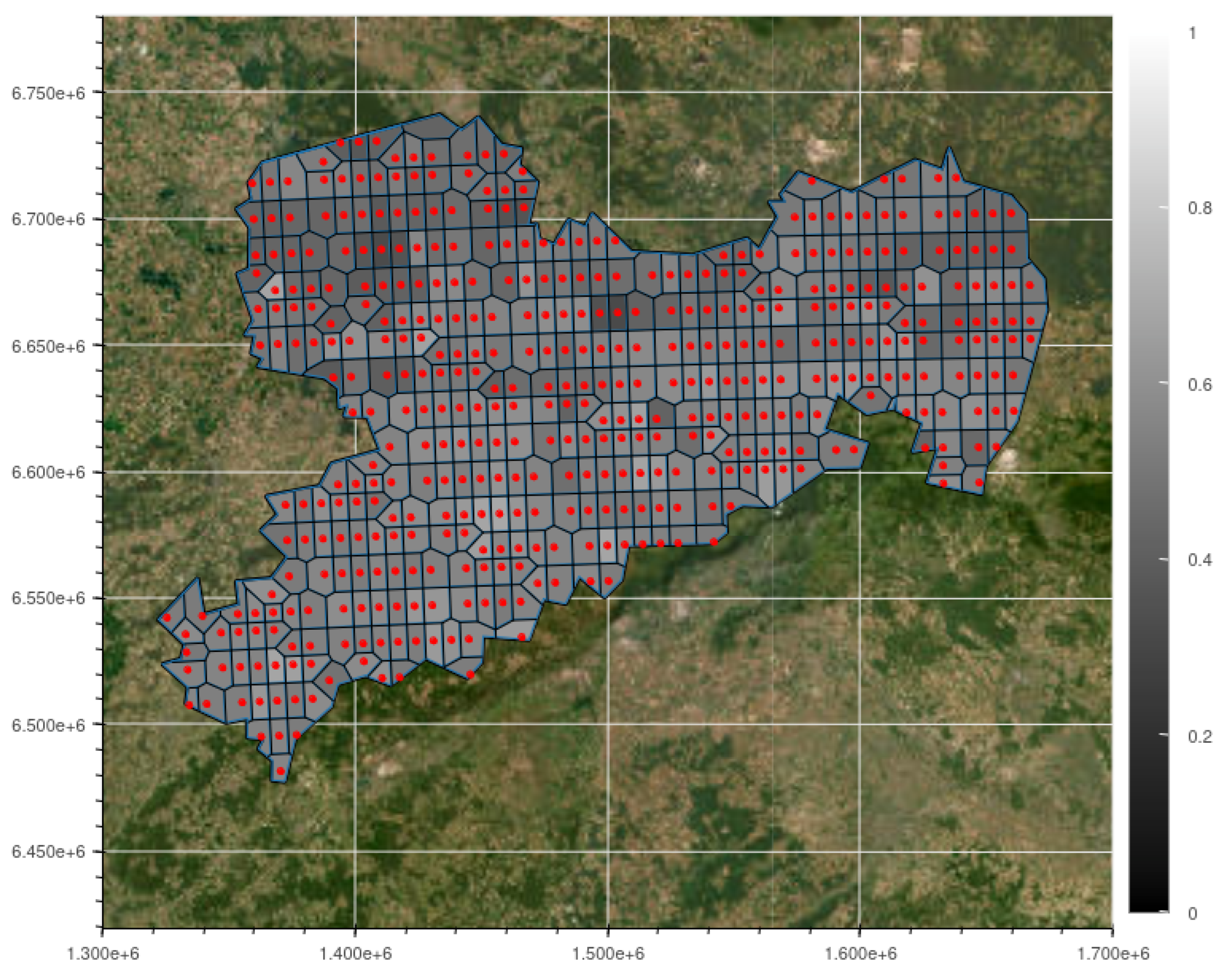
As stated in Section 1, a minor goal of this work is to get an understanding in local differences on a small scale. Some insights are given in Figure 1, Figure 4 and Figure 5. In these figures some of the variation within the Saxon data is shown. The SPEI-values are very similar with only small differences between the 25th and 75th percentiles. The plotted AGGDs show local differences with regards to temperature. The biggest difference appears within the frost data, where the duration of the yearly frost free period in two locations shows a completely different trend. In order to evaluate the effect of data selection on the regression models, we create a regression model for every single available set of data with the same features as described in Section 4.2, for every available crop. A resulting overview is given in Figure 10, which depicts a map of Saxony with all 448 locations included in the dataset, represented as red dots. Using these locations and the Saxon border, a Voronoi diagram is created, assigning a region to each location. The regions are colored according to the R 2 -values of the corresponding regression model. There is large variation between the quality of the different models with R 2 -values ranging from 0.3 to 0.7 There is no clear pattern as to where the best fits are located. Generally, the northern region contains weaker fits.
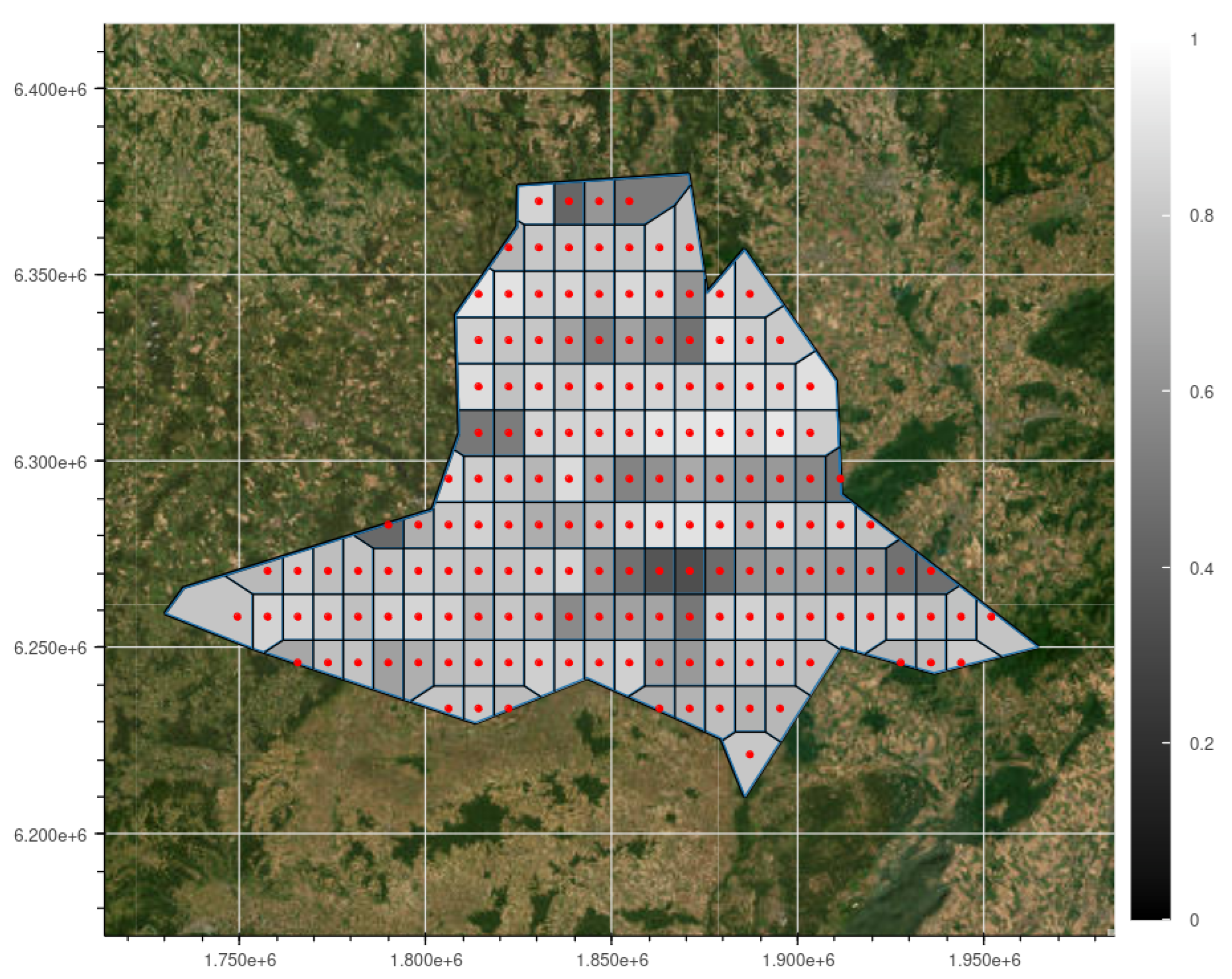
Using the same methodology, a map is also created for the South-Moravian Region, shown in Figure 11. The R 2 -values for South-Moravia range from 0.3 to 0.9 . While the lower bound for calculated R 2 -values is similar to those calculated for Saxony, the mean values are much higher, which is also immediately visible due to the coloring. A major reason for this difference is the shorter length of the timeseries containing the crop yields for South-Moravia, which leads to a higher relative dimensionality of the regression.
We compare the quality of the 448 regression models for Saxony with that of the ensemble model, which was computed by using the medians of all 448 timeseries. The results for the ensemble model were given in Table 7. A short comparison between the ensemble model and the single models is displayed in Table 8: The column R 2 -Saxony shows the values of the ensemble model, the values in R 2 -Minimum column are the minimal values for either of the single models, and analogically, the R 2 -Maximum and R 2 -Median columns shows the maximal/median values for either of the single models. As can be observed, the best single model is always at least slightly better than the ensemble model. However, in contrast, the worst model always does much worse. The median of the single models tends to do worse if the ensemble model yields good results. If the ensemble model delivers low R 2 -values, the median of the single models will most likely be slightly higher. However, if this occurs, the results are generally low and therefore do not provide insights. This experiment was done for all Saxon crops, with no significant differences between the described behavior of the models.
Another aspect is the transferability of best or worst location models - that is, whether locations with data that lead to the best/worst regression models for one crop would lead to equivalent models for other crops. To conduct a more thorough investigation, all models for the various crops were compared with regards to the locations of the best fits. The results show no underlying pattern as to where the best/worst models are located.

5. Discussion

We created LSTMs with SPEIs as input data for scales 1 and 3. We conclude that, with the amount of data we have, a LSTM with scale 1 cannot provide results that are accurate enough to give precise predictions for the near future. The trained nets lack accuracy and robustness when predicting unknown data. The LSTMs trained with scale 3 on the other hand are extremely precise, which suggests that this may be due to overfitting. Considering that the scale of the SPEI only has a very small effect on the sample size, one possible explanation for overfitting could be a reduced variation across all datasets, which would be caused by the sliding window part of the upscaling. Another possibility is that the LSTMs recognised underlying relations between SPEI-values for corresponding timeframes and therefore simply give good results. We leave the investigation of whether the results stem from overfitting to future work. Otherwise this method looks very promising and can be used to gain insights into short-term drought events which can then be used by agricultural producers in the planning stage for the relevant time period.
The results for the studied crop yields remain inconclusive, as the correlation between yields and drought indicates that yields improve with drier conditions. What can be deduced from this is the assumption, that the droughts in recent years had a smaller effect on most crops than technological advancements that were made in our areas of interest. Therefore, we also assume that in the following years droughts are not likely to cause major yield losses. The only exception observed on the Saxon data is the silage maize production, where a small negative effect of droughts during spring months is indicated. The findings by Mansoor Maitah and Maitah [10], who stated July and August as the most critical months for maize in the Czech Republic, can therefore not be replicated with the Saxon data. One major risk for future crop yields might be the reduction in groundwater reserves. This was not measured in our data, but is a topic for future research.
Simple correlation methods are easy to compute and easy to understand, but are susceptible to false results, such as high correlations caused by chance or low correlations caused by incomplete information. Therefore, to increase the accuracy of calculations that measure the effect of climatic factors on crop yield, we propose to add occurrences of spring frosts, as well as GDD-timeseries, as we have done in Table 7. This approach combines weak predictors for crop yields into a single, stronger predictor. We strongly recommend to include temperatures lower than 0°C for future research into effects of frost on agricultural yields, as the results presented in Table 7 indicate much larger effects for strong frost events on most crops.
Another topic for future research would be to predict crop yields based on climatic factors for single fields or smaller areas. This was not included in our research as these data were not not available to us. While predictions using smaller regions for timeseries gave weaker results, this might change if the yield resolution becomes higher.

Author Contributions

Conceptualization, A.K. and J.S.; methodology, J.S.; software, J.S.; validation, A.K., J.S.; formal analysis, J.S.; investigation, A.K. and J.S.; resources, A.K.; data curation, J.S.; writing—original draft preparation, A.K. and J.S.; writing—review and editing, A.K. and J.S.; visualization, J.S.; supervision, A.K.; project administration, C.Z.; funding acquisition, C.Z. All authors have read and agreed to the published version of the manuscript.

Funding

This work was supported by the STARGATE project, funded by the European Union’s Horizon 2020 research and innovation programme under grant agreement no. 818187.

Data Availability Statement

The datasets presented in this article are not readily available because they were downloaded from a commercial platform. Requests to access the datasets should be directed to meteoblue. In case meteoblue grants access, the authors declare that they will provide access to the data downloaded and curated datasets.

Acknowledgments

meteoblue data is provided within the European Union’s Horizon 2020 Research and Innovation Programme under grant agreement No. 818187 (https://www.stargate-h2020.eu)

Conflicts of Interest

The authors declare no conflict of interest.

Abbreviations

The following abbreviations are used in this manuscript:
SPEI Standardised Precipitation-Evapotranspiration Index
SPI Standardised Precipitation Index
LSTM Long Short-Term Memory
GDD Growing Degree Days
AGGD Accumulated Growing Degree Days

References

  1. Hochreiter, S.; Schmidhuber, J. Long short-term memory. Neural computation 1997, 9, 1735–1780. [Google Scholar] [CrossRef] [PubMed]
  2. Vicente-Serrano, S.M.; Beguería, S.; Lopez-Moreno, J.I. A Multiscalar Drought Index Sensitive to Global Warming: The Standardized Precipitation Evapotranspiration Index. Journal of Climate 2010. [Google Scholar] [CrossRef]
  3. Rhee, J.; Im, J. Meteorological drought forecasting for ungauged areas based on machine learning: Using long-range climate forecast and remote sensing data. Agricultural and Forest Meteorology 2017. [Google Scholar] [CrossRef]
  4. Sobia Wassan, Chen Xi, N.J.; Binte-Imran, L. Effect of frost on plants, leaves, and forecast of frost events using convolutional neural networks. International Journal of Distributed Sensor Networks, 2021.
  5. Weyn, J.A.; Durran, D.R.; Caruana, R.; Cresswell-Clay, N. Sub-Seasonal Forecasting With a Large Ensemble of Deep-Learning Weather Prediction Models. Journal of Advances in Modeling Earth Systems 2021. [Google Scholar] [CrossRef]
  6. ECMWF. https://www.ecmwf.int/. Accessed: 2024.
  7. Dikshit, A.; Pradhan, B.; Huete, A. An improved SPEI drought forecasting approach using the long short-term memory neural network. Journal of Environmental Management 2021, 283, 111979. [Google Scholar] [CrossRef] [PubMed]
  8. Jamieson, P.D.; Martin, R.J.; Francis, G.S. Drought influences on grain yield of barley, wheat, and maize. New Zealand Journal of Crop and Horticultural Science 1995. [Google Scholar] [CrossRef]
  9. Kolář, P.; Trnka, M.; Brázdil, R.; Hlavinka, P. Influence of climatic factors on the low yields of spring barley and winter wheat in Southern Moravia (Czech Republic) during the 1961–2007 period. Springer-Verlag Wien, 2013. [Google Scholar]
  10. Mansoor Maitah, K.M.; Maitah, K. Influence of precipitation and temperature on maize production in the Czech Republic from 2002 to 2019. Scientific Reports 2021. [Google Scholar]
  11. Labudová, L.; Labuda, M.; Takáč, J. Comparison of SPI and SPEI applicability for drought impact assessment on crop production in the Danubian Lowland and the East Slovakian Lowland. Springer-Verlag Wien, 2016. [Google Scholar]
  12. Zheng, B.; Chapman, S.C.; Christopher, J.T.; Frederiks, T.M.; Chenu, K. Frost trends and their estimated impact on yield in the Australian wheatbelt. Journal of Experimental Botany 2015. [Google Scholar] [CrossRef] [PubMed]
  13. Frederiks, T.; Christopher, J.; Harvey, G.; Sutherland, M.; Borrell, A. Current and emerging screening methods to identify post-head-emergence frost adaptation in wheat and barley. Journal Of Experimental Botany 2012. [Google Scholar] [CrossRef] [PubMed]
  14. Kukal, M.S.; Irmak, S. Agro-Climate in 20th Century: Growing Degree Days, First and Last Frost, Growing Season Length, and Impacts on Crop Yields. Scientific Reports 2018. [Google Scholar] [CrossRef] [PubMed]
  15. Wypych, A.; Sulikowska, A.; Ustrnul, Z.; Czekierda, D. Variability of growing degree days in Poland in response to ongoing climate changes in Europe. International Journal of Biometeorology 2017. [Google Scholar] [CrossRef] [PubMed]
  16. Trnka, M.; Olesen, J.; Kersebaum, K.; Skjelvåg, A.; Eitzinger, J.; SEGUIN, B.; Peltonen-Sainio, P.; Rötter, R.P.; Iglesias, A.; Orlandini, S.; Dubrovský, M.; HLAVINKA, P.; Balek, J.; ECKERSTEN, H.; Cloppet, E.; Calanca, P.; Gobin, A.; Vučetić, V.; Nejedlik, P.; ŽALUD, Z. Agroclimatic conditions in Europe under climate change. Global Change Biology 2011, 17, 2298–2318. [Google Scholar] [CrossRef]
  17. Potopová, V.; Štěpánek, P.; Možný, M.; Turkott, L.; Soukup, J. Performance of the standardised precipitation evapotranspiration index at various lags for agricultural drought risk assessment in the Czech Republic. Agricultural and Forest Meteorology 2014. [Google Scholar]
  18. Statistical Yearbook of the Jihomoravský Region 2020. https://www.czso.cz/csu/czso/statistical-yearbook -of-the-jihomoravsky-region-2020. Accessed: 2024.
  19. Saxon State Ministry of Energy, Climate Protection,Agriculture and the Environment (SMEKUL). Agriculture and food industry 2023, 2023.
  20. meteoblue. meteoblue.com. Accessed: 2024.
  21. Statistisches Landesamt Sachsen. https://www.landwirtschaft.sachsen.de/ertraege-von-getreide-und-raps -37266.html. Statistisches Landesamt Sachsen, Accessed: 2024.
  22. drought-Indexes. https://www.drought.gov/data-maps-tools/source-code-climate-and-drought-indices- python-spi-spei-pet. Accessed: 2024.
  23. McKee, T.B.; Doesken, N.J.; Kleist, J. The Relationship of Drought Frequency and Duration to Time Scales. Eighth Conference on Applied Climatology 1993. [Google Scholar]
  24. Wells, N.; Goddard, S.; Hayes, M. A Self-Calibrating Palmer Drought Severity Index. Papers in Natural Resources 2004. [Google Scholar] [CrossRef]
  25. Python package for climate indices. https://climate-indices.readthedocs.io/en/latest/. Accessed: 2024.
  26. James, G.; Witten, D.; Hastie, T.; Tibshirani, R. An Introduction to Statistical Learning; Springer Texts in Statistics, 2014.
  27. Graves, A. Supervised Sequence Labelling with Recurrent Neural Networks; Studies in Computational Intelligence, Springer, 2012.
  28. Keras (Python package). https://keras.io/. Accessed: 2024.
  29. Tensorflow. https://github.com/tensorflow/tensorflow. Accessed: 2024.
  30. McMaster, G.S.; Wilhelm, W. Growing degree-days: one equation, two interpretations. Agricultural and Forest Meteorology 1997, 87, 291–300. [Google Scholar] [CrossRef]
Figure 1. SPEI time series for scales of 1 month (a) and 6 months(b) for the South-Moravian region between 1990 and 2021. The plots include the medians as well as the 25 and 75 percentiles of all available time series of this region.
Preprints 108996 g001
Figure 2. Architecture of an LSTM unit (FC = fully connected) [1]
Preprints 108996 g002
Figure 3. Comparison of raw and detrended yields for wheat in Saxony from 1990 2021
Preprints 108996 g003
Figure 4. Trends of duration for frost-free periods. Figures (a) and (b) show the yearly number of consecutive days without frost as dots with a regression line. The difference between both figures is the location from where the data was collected.
Preprints 108996 g004
Figure 5. Accumulated Growing Degree Days for Saxony in 1990 (a) and 2020 (b). The different plots visualize the data for different locations.
Preprints 108996 g005
Figure 6. Plot containing the training and test losses for a continuum of input lengths. The train losses are very small for input sequences that include 2 or more values. The test losses are also small for input sequences of 2 or longer, but are significantly larger than training losses if the sequences are roughly longer than 10 values. Most test losses vary between 0.01 and 0.2 .
Preprints 108996 g006
Figure 7. Comparison of prediction results from LSTMs which were trained with scale 1 (left columns) and scale 3 (right column). The first row shows results from the training data, the second row from the validation data and the third row from the test data.
Preprints 108996 g007
Figure 8. Heatmaps for the correlation of SPEI timeseries seperated by months with timeseries of yearly crop yields. The heatmaps in the first row show the values for wheat production Saxony, respectively South-Moravia. The second row consists of heatmaps for sugar beet. The third row shows a heatmap for silage maize production in Saxony and vine in South-Moravia.
Preprints 108996 g008
Figure 9. Heatmaps for the correlation of SPEI timeseries seperated by months with timeseries of detrended yearly crop yields.
Preprints 108996 g009
Figure 10. Map of Saxony with R 2 -values of the regression method described in Section 3.3 with wheat as crop. The map is split into regions as a Voronoi diagram, with each dot marking a location with an available set of timeseries for SPEI, frost and GDD. For this figure the SPEI 6-values from March serve as input into the regression, along with the frostdays calculated by using a threshold of 5 C , and the GDD with a base temperature of 3 C . The resulting R 2 -values are within 0.3 and 0.7 .
Preprints 108996 g010
Figure 11. Map of South-Moravia with R 2 -values of the regression method described in Section 3.3 with wheat as crop. The methodology is identical to Figure 10. The resulting R 2 -values are within 0.3 and 0.9 .
Preprints 108996 g011
Table 2. Metrics of input SPEI
Scale Mean Variance Autocorrelation
SPEI 1 -0.3 1.15 2.97
SPEI 2 -0.39 1.18 2.05
SPEI 3 -0.44 1.17 1.9
SPEI 6 -0.55 1.26 1.92
Table 3. Training data example
x 0 x 1 x 2 x 3 y
1.09126734 0.13360752 1.41027385 1.20590687 1.43453393
0.13360752 1.41027385 1.20590687 1.43453393 1.25543713
1.41027385 1.20590687 1.43453393 1.25543713 0.18184788
Table 4. Training data example with added noise
x 0 x 1 x 2 x 3 y
1.1717148 0.16360395 1.38089293 1.2080818 1.43453393
0.22412484 1.41258663 1.17648276 1.43466805 1.25543713
1.32318195 1.10849753 1.44886319 1.26732118 0.18184788
Table 5. Overview over losses for different LSTMs, which are trained with varying settings specified in the first column. The LSTMs are either trained with SPEI of scale 1 or 3. The data is either split spatially, meaning the training data consists of a subset of all full timeseries, or temporally, meaning the training data consists of all timeseries with data from a few years missing. For the temporal split the data used for validation is either removed from the end of the timeseries (rows 3 and 4), or from the start of the timeseries, which is indicated as temporal inverted.
LSTM Loss Training Saxony Loss Test Saxony Loss Test 1 Loss Test 2
Scale 1; spatial 0.04 0.10 0.74 1.12
Scale 3; spatial 0.006 0.006 0.006 0.006
Scale 1; temporal 0.13 1.56 1.20 1.54
Scale 3; temporal 0.006 0.01 0.01 0.01
Scale 1; temporal inverted 0.09 1.28 1.21 1.53
Scale 3; temporal inverted 0.004 0.93 0.08 0.13
Table 6. Overview over variance of the data. The first value of each pair gives the variance of the ground truth SPEI-data and the second value the variance of the respective data fit. The LSTMs used to record this data are the same as in Table 5.
LSTM Training Saxony Test Saxony Test 1 Test 2
Scale 1; spatial 0.78/0.97 0.97/1.00 1.07/0.70 1.09/0.53
Scale 3; spatial 1.14/1.00 1.00/1.05 1.10/0.98 1.10/0.98
Scale 1; temporal 1.03/0.83 0.83/0.29 1.26/0.50 1.27/0.39
Scale 3; temporal 1.07/0.94 0.94/0.71 1.10/1.00 1.10/0.98
Scale 1; temporal inverted 1.17/0.94 0.94/0.54 1.26/0.61 1.27/0.52
Scale 3; temporal inverted 0.95/0.85 0.85/0.31 1.10/0.85 1.10/0.82
Table 7. R 2 -values of crop yields calculated with a polynomial regression of 2nd order with a combination of SPEI, frost days and GDD. T b a s e consists of base-temperatures, which are needed for plant growth, for the respective crops. The value in the frost column is the temperature used to determine whether a given day counts as a frost day. The values for SPEI 3, respectively SPEI 6 are the highest R 2 -values of the corresponding regressions. The column with relevant months gives the months in which the highest R 2 -values of the regressions are achieved.
Crop T b a s e Frost SPEI 3 SPEI 6 Relevant Months
Wheat 4 . 5 C 5 C 0.74 0.71 February-April
Winter Wheat 4 . 5 C 5 C 0.74 0.71 February-April
Rye 4 . 5 C 1 C 0.41 0.39 February-April
Winter Barley 4 . 5 C 5 C 0.62 0.73 January-April
Spring Barley 4 . 5 C 5 C 0.67 0.65 February-May
Oat 4 . 5 C 5 C 0.56 0.50 February-April
Triticale 4 . 5 C 5 C 0.43 0.42 February-March
Grain Maize 10 C 0 C 0.63 0.64 May-August
Potatoes 8 C 0 C 0,54 0.56 January-June
Sugar Beet 4 . 5 C 0 C 0.66 0.74 January-June
Rape 4 . 5 C 2 C 0.61 0.57 August/whole year
Silage Maize 10 C 0 C 0.73 0.69 August-October
Grain 4 . 5 C 5 C 0.73 0.74 February-April
Table 8. Table with a subset of R 2 -values from regressions as described in Section 3.3. For this case the SPEI 3 was used, along with a frost threshold of 5 C and a base temperature of 4 . 5 C . The first column with values shows R 2 -values for the regression with the inputs being the medians of the Saxon data. The other columns show minimum, maximum and median for the regression values, with every single timeseries set as input.
Month R 2 -Saxony R 2 -Minimum R 2 -Maximum R 2 -Median
February 0.74 0.4 0.75 0.54
March 0.65 0.31 0.68 0.54
April 0.54 0.28 0.63 0.46
May 0.44 0.15 0.68 0.37
Disclaimer/Publisher’s Note: The statements, opinions and data contained in all publications are solely those of the individual author(s) and contributor(s) and not of MDPI and/or the editor(s). MDPI and/or the editor(s) disclaim responsibility for any injury to people or property resulting from any ideas, methods, instructions or products referred to in the content.
Copyright: This open access article is published under a Creative Commons CC BY 4.0 license, which permit the free download, distribution, and reuse, provided that the author and preprint are cited in any reuse.
Prerpints.org logo

Preprints.org is a free preprint server supported by MDPI in Basel, Switzerland.

Subscribe

© 2024 MDPI (Basel, Switzerland) unless otherwise stated