Preprint
Article

Sensitivity Analysis and Filtering of Machinable Parts Using Density-Based Topology Optimization

Altmetrics

Downloads

109

Views

40

Comments

0

A peer-reviewed article of this preprint also exists.

Submitted:

12 June 2024

Posted:

13 June 2024

You are already at the latest version

Alerts
Abstract
Topology optimization has become a very popular design tool when an optimum design with a concrete objective and subjected to several restrictions is searched. However, the resultant shape of the optimization process isn’t usually easy to manufacture with a typical manufacturing method as machining, being necessary an interpretation and validation of the result; besides, some parameters can be chosen, and the final shape is directly dependent on them. In this paper, a sensitivity analysis of the main parameters involved in 3D topology optimization, the penalization and the filter radius, is carried out for the concrete case of the density-based method, analyzing how manufacturable the results are for 3 axis machining. Also, a new filter and method is proposed for obtaining highly manufacturable and low interpretable parts. The main aim of the study is to help designers to choose the more appropriate parameters and showing what they must have into account for obtaining the desired optimized shapes. Note that the density-based topology optimization method has been chosen due to its popularity in commercial packages, so the conclusions may have direct applications in designers’ work. Finally, the results of the study are verified through different cases for checking the validity of the conclusions.
Keywords: 
Subject: Engineering  -   Mechanical Engineering

1. Introduction

Topology optimization (TO) is a design tool for obtaining optimal shapes with known conditions, based on the optimization problem definition; In other words, it aims to achieve the best possible result for a given function while applying specific constraints. Topology optimization has been increasingly used during the last years, as well as the research on the topic and the development of commercial software for obtaining topology parts, as mentioned by Shiye and Jiejiang [1]. Nevertheless, the foundations of TO theory were established over a century ago [2], with major applications to the actual theory with the guidelines developed by Dorn [3]. Years later, the computerization of topology optimization arrived [4] and later further applications in the digital era [5].
In this epigraph, a brief explanation of the density-based TO is presented in order to show the used methods, solving techniques and filters; as well as the application of the studied parameters. The values of these and MatLab® codes are provided for replicating the results of the study, which can be applied to the main topology optimization codes discussed in the literature [6,7]. This chapter is divided in two sections: one related to the used topology optimization method, and other related to the filters oriented towards subtractive manufacturing.

1.1. Density-Based Topology Optimization
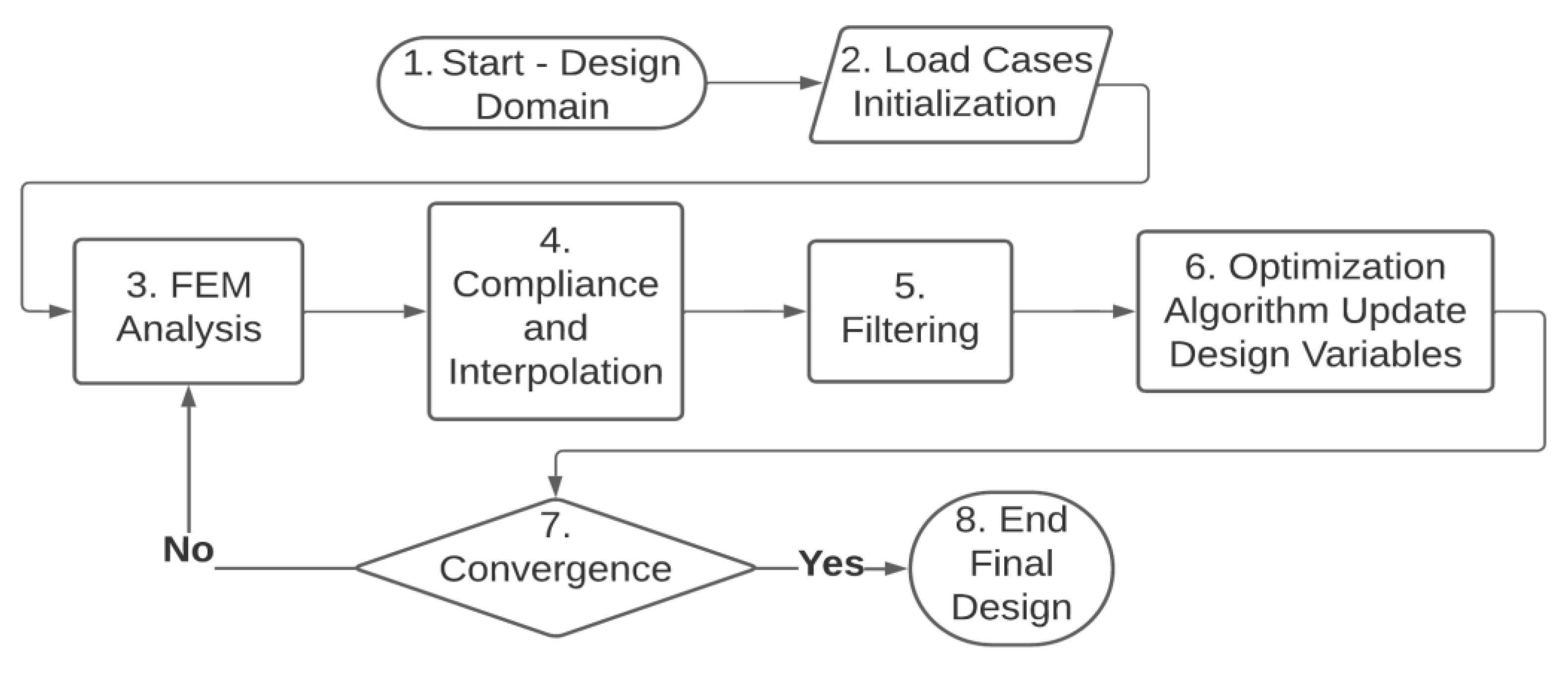
The density-based approach starts from a design domain that is discretized using nodes and elements. This design domain is the maximum space (line, surface or volume) where the final design could exist, and a density value is assigned to each element of the discretized design domain, hence it is parametrized by this density. The density value is not binary, so it can vary from 0 (void) to 1 (solid), and this value is applied by using an interpolation function [8,9]. The use of only black and white elements easily leads to an ill-posed result [10]. Many solutions have been proposed [11,12,13], but none are totally satisfactory. An interesting proposal was to include not only binary values for the density of each element [9,14], those values being chosen automatically following a power rule (Zhou & Rozvany, 1991): the interpolation scheme, that will be explained later in this manuscript.
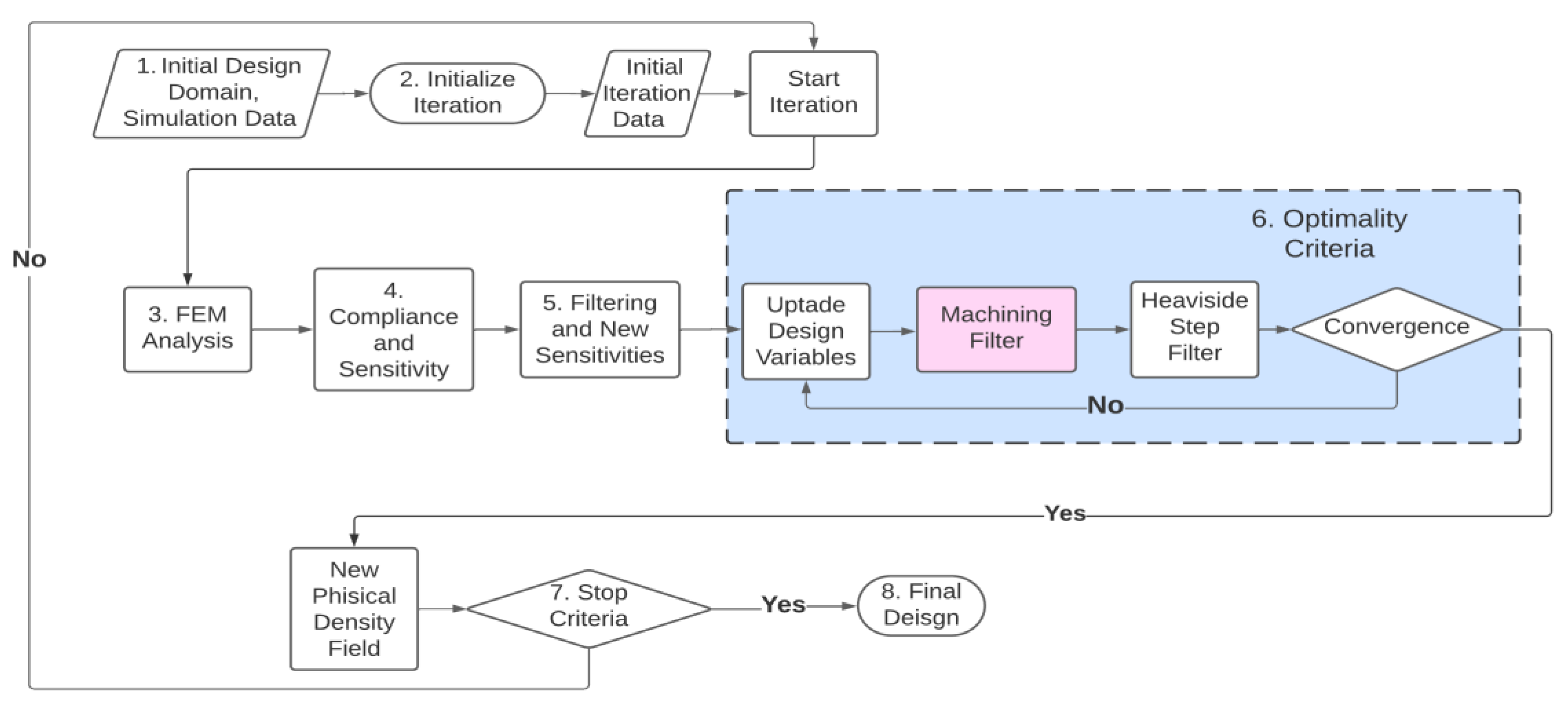
The used density-based approach is extensively described in several studies [6,16], and follows the simplified flowchart showed in Error! Reference source not found., where every step is numbered for future references.
Figure 1. Simplified flowchart of the density-based topology optimization process.
Preprints 109083 g001
In this study, special attention is given to levels 4 and 5 of the flowchart in Error! Reference source not found., as these processes involve the parameters under study. Specifically, for the interpolation in level 4, Solid Isotropic Material with Penalization method (SIMP) is utilized; additionally, a density filter is employed as the filtering technique in level 5.

1.2. Interpolation Scheme, the SIMP

The SIMP is based on the relation of the stress state of every element with its relative density. The formulation is included in Equation (1):
E i = E x i = E m i n + x i p ( E 0 E m i n )
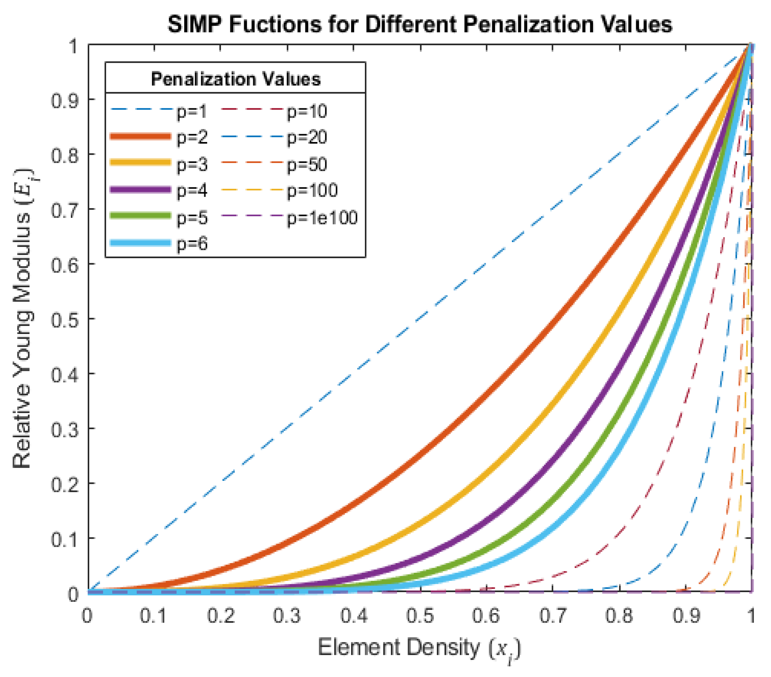
Being E i the relative Young Modulus of each element (calculated using FEM and representing the stress state of the element; note that it is also dependant on its degrees of freedom), E m i n as the almost zero elastic modulus of void material for avoiding mathematical incompatibility issues, E 0 as the elastic modulus of the original material, x i as the relative density of the element i , and p as the penalization factor. This penalization factor is one of the parameters to use in the sensitivity analysis of this manuscript. According to the Equation (1), it is evident that a higher p will result in a more binary outcome (Jiang, 2017), corresponding to the graph of a power rule function presented in Error! Reference source not found..
Figure 2. Graphical representation of the SIMP interpolation power rule for penalization values between 1 and 100.
Preprints 109083 g002
SIMP represents a robust, highly configurable, and computationally efficient scheme. It does not require homogenization and is adaptive to various design conditions and constraints. Due to these advantages, SIMP is chosen as the initial interpolation scheme for the research conducted in this work. However, using SIMP comes with challenges such as dealing with intermediate densities, mesh dependency, and potential non-convergence [17].

1.3. Filtering, the Density Filter

The density-based method employs finite element analysis (step 3 in Error! Reference source not found.) and the SIMP method to assign each element a relative density value ranging from 0 to 1. The classical approach is finding a black-and-white layout (zeros and ones) that minimizes the compliance of the structure, subjected to a maximum volume fraction in relation to the original volume of the design domain [6].
The use of purely black and white elements often leads to an ill-posed result [10]. Many solutions have been proposed [11,12,13], but none have proven entirely satisfactory. An interesting proposal was to include non-binary density values for each element [9,14], automatically determined through a power rule [15], the SIMP.
Nonetheless, even with SIMP, mesh dependency, checkerboard, ill-posed or local minima results can still arise [18]. To address these issues the density filter [19] is employed in this study. A basic formulation of this filter is presented in Equation (2):
x ~ i = j ϵ N i H i j v j x j j ϵ N i H i j v j
where x ~ i is the filtered density of an element, N i representsthe neighborhood of a specific element, v j is the volume of the element i, and H i j is a weight factor. The neighbourhood of an element is defined as all the elements whose centre is within a certain distance R from the centre of the element in analysis. This can be defined as Equation (3):
N i = j : d i s t ( i , j ) R
And the weight factor H i j can be defined as Equation (4):
H i j = R d i s t ( i , j )
Being j always inside the neighbourhood N i and representing the geometric center of each element. The constant R is defined as the filter radius, and is the second parameter used in the sensitivity analysis throughout this paper. Now, x ~ i from Equation (2), known as the filtered density of the element, is substituted in the SIMP (Equation (1)) as Equation (5):
E i = E x ~ i = E m i n + x ~ i p ( E 0 E m i n )

1.4. Study Description and Novelty

As density-based TO is the most popular method in the commercial packages, such as Altair Hyperworks suite [20], Ansys suite [21], Dassault Systèmes suite [22] or PTC suite [23]; this manuscript aims to analyze the two main parameters involved in the optimization process: penalty and filter radius. The objective of this study is to determine the best parameters for obtaining manufacturable results with minimal interpretation for 3 axis machining. This research aims to assist designers in making informed decisions and save time in preprocessing and simulation phases.
A wide range of values is considered fo the mentioned parameters, and calculation times, discreteness and machinability of the results are presented. It is important to note that other studies [1,24,25] make remarkable contributions in this area, but none of them are specifically oriented to a concrete manufacturing method and are often limited to a short set of values for the studied parameters, they don’t take into account the mesh depencency, or study only the 2D case. Other works [26,27] concentrate on achieving these manufacturable parts by adding filters and additional constraints to the TO process, but a more direct aplication is searched in the present paper.
The given text describes the development of a novel analysis tool that can assess the machinability of a part for a 3-axis machine. This tool is later applied as a filter to automatically modify the non extra-constrained part, making it more machinable and less interpretable. A MatLab® will be provided for the use of the scientific and designers community, and for the replication of the research results.
The structure of the paper is organized as follows:
  • The initial section discusses the chosen parameters values criterion is, along with the load case and material parameters of the main study case for the sensitivity analysis.
  • Following that, the parameters used for analyzing the results are exposed and explained, with particular emphasis in the measure of the discreteness and the evaluation of the machinability,
  • Subsequently, results of the 92 simulations are exposed and analyzed, being able to obtain the conclusions related to the aim of the study.
  • The machining filter is presented and verified through different verification tests.
  • Finally, the conclusions drawn from the study and potential avenues for future research are presented.

2. The Case Study

2.1. Parameters’ Values Selection Criterion

The text highlights that the filter radius ( R ) and penalization ( p ) are the two main parameters being analyzed. These parameters should not be chosen arbitrarily but require careful consideration to achieve a satisfactory outcome.
For penalization p , previous studies [1,24] indicate that a minimum value of 3 should be used for isotropic materials with a Poisson Ratio ν ~ 1/3, within the defined topology optimization method. The relative density of each element, as shown in Error! Reference source not found., follows a power rule, and it is observed that higher penalization values lead to sharper trends towards either 0 or 1 density. However, as the penalization increases, the differences in the results become smaller [25]. To analyze the parameter’s impact, values ranging from three (3) to six (6), inclusive, with increments of one (1) are chosen based on previous studies [1,24] indicate. By using these values, it becomes possible to observe the transitional changes in the resultant shapes when larger penalization values are employed.
For filter radius R , the values have been taken from different scopes, and they are summarized in Table 1. These sources include:
  • Values used in other mentioned studies (OS).
  • Values derived from the Euclidean distance between the element under analysis and the neighboring layer of elements (ED).
  • Large estimated values intended to observe the behavior of the method with extreme values (LV).
The values of the filter radii in Table 1 have been rounded to reduce computation time. This approach was chosen because the filter radius is a highly recurrent value throughout the process. Rounding the number to a value that does not overlap with the next filter radius value does not impact the result.

2.2. Case Study Description and Material
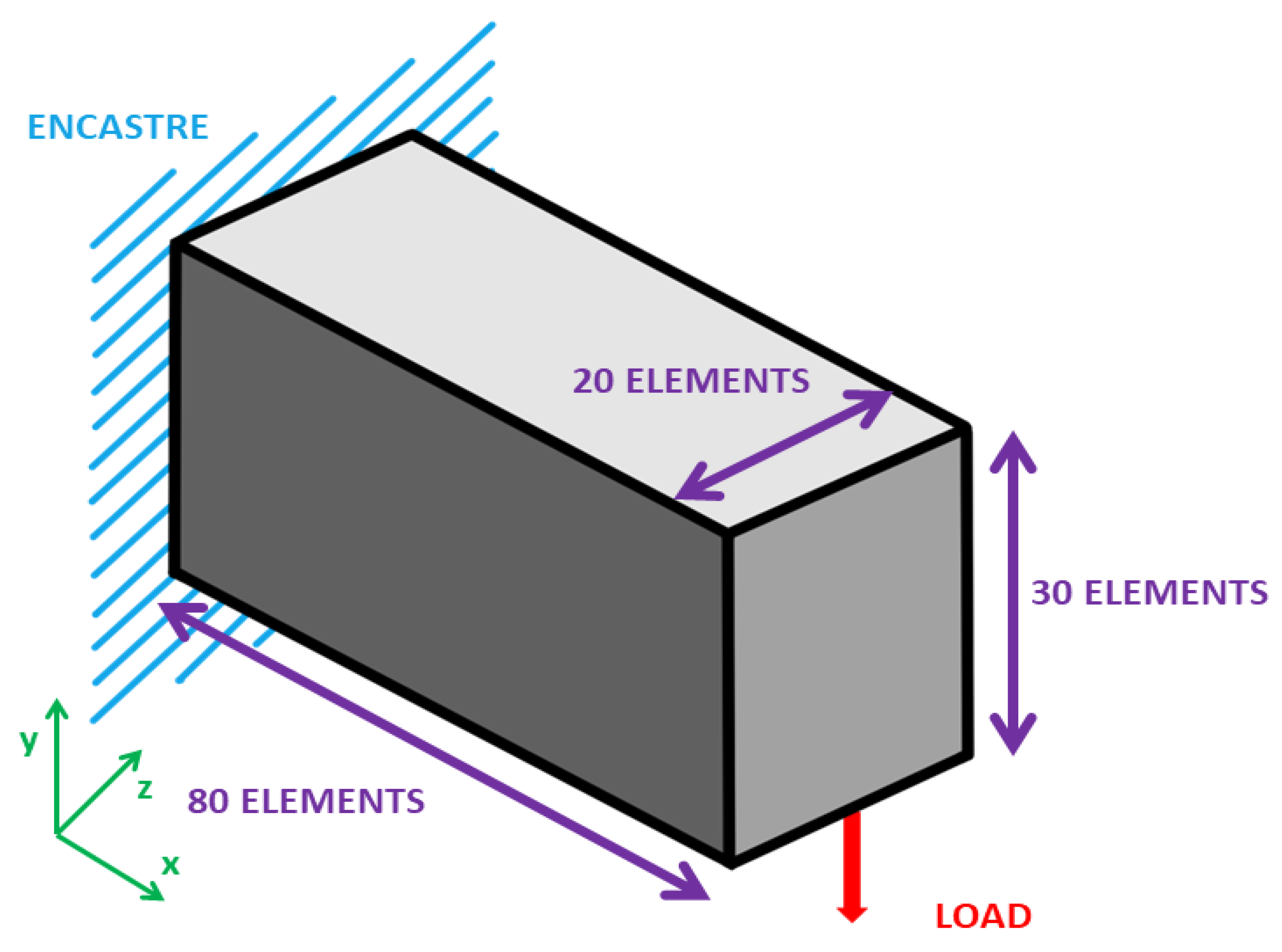
One aim of the study is to analyze parameters in a 3D structure, so the initial design space needs reliable dimensions in the x, y, and z directions. The typical load case involves minimizing compliance with a volume fraction constraint in a cantilever beam with a vertically applied distributed force. In this study, a point force (tip load) is used to emphasize the 3D nature of the case.
Considering that the element size is 1 in all directions, the initial design space consists of 80 elements in the x direction, 30 elements in the y direction, and 20 elements in the z direction. This choice helps generate fewer flat shapes in the optimization result. Error! Reference source not found. illustrates the case study with the applied load and the number of elements.
For this study, a volume fraction of 0.2 is applied, and a material with a Poisson Ratio (ν) of 0.3 is used. The value of E m i n in Equation 1 is set to 10−9 which is close enough to zero to avoid affecting calculations and prevent mathematical singularities; and E 0 is set to 1, which is a typical used value in mentioned previous studies for researching and reducing calculation time. These properties are chosen for comparing the results to other studies [1,24] and having a direct application in the know and accesible MatLab® codes [6,7].
Figure 3. Study Load Case and Design Domain.
Preprints 109083 g003
The convergence is achieved when the maximum change in the density of any element between two consecutive iterations is less than 0.01, which is the recommended value based on the experience of previous studies [6].

2.3. Parameters for the Results Analysis

The sensitivity analysis aims to evaluate the machinability by exploring different filter radii and penalties to assist designers in their projects. The parameters extracted from the simulation results are intended to objectively demonstrate this characteristic. These parameters include the number of iterations, time per iteration, measure of non-discreteness, and machinability.
The number of iterations and time per iteration are directly obtained from MatLab® and will be presented in the subsequent section. However, further explanations are needed for the measure of non-discreteness and machinability, which will be provided below.

2.3.1. Measure of Non-Discreteness

Discreteness refers to a global characteristic of the final design, indicating how binary the result is with distinct void ( x ~ i =0) and solid x ~ i =1) elements. This parameter is important because the representation of the result includes only elements with density x ~ i above a threshold (in this case, 0.5). Consequently, there are elements that do not appear in the final design but still contribute to compliance, and their significance increases as the discreteness of the result grows. Since the designer needs to interpret the shape displayed in the topology optimization (TO) result, and one objective of the study is to obtain easily interpretable components, it is essential to control and minimize the discreteness.
To analyze the characteristic of discreteness, Sigmund introduced a tool called the measure of non-discreteness ( M n d ), which is widely utilized in the investigation of this matter [28]. The measure of non-discreteness is represented by Equation 6:
M n d = e = 1 N 4 x ¯ e ( 1 x ¯ e ) N × 100 %
In the provided context, N refers to the ID of each element in the design domain. The parameter M n d represents the measure of non-discreteness. It should be noted that the lower the value of M n d , the more binary the result of the analysis is, indicating a higher level of discreteness.

2.3.2. Machinability

Here, the machinability of the optimized shape is analyzed by assessing the accessibility of a hypothetical tool to each frontier element. A frontier element refers to the last element with a density higher than the chosen threshold. This analysis involves an element-by-element evaluation.
To initiate the analysis, the set of elements exceeding the selected density threshold is divided into distinct groups:
  • The external layer (EL): Comprising all the elements located on the boundaries of the design domain. These elements are always accessible because they do not have any solid interface with the exterior.
  • The core layers (CL): Representing the internal solid region, consisting of all the elements forming the shape of the part excluding the frontier elements.
  • The frontier layer (FL): Consisting of the elements above the density threshold and located between the solid and void phases.
The frontier layer (FL) can be determined by considering that it includes all the elements exceeding the threshold, but not belonging to the E L or C L groups, as stated in Equation (7):
n = 1 n N = e = 1 e E L + c = 1 c C L + f = 1 f F L
The F L is divided into three distinct groups in the subsequent step. These groups are based on the accessibility of the elements for a tool and their machinability. The groups are as follows:
  • Elements directly accessible for a tool: These are the elements within the FL that can be readily machined using a tool.
  • Elements not directly accessible but machinable by machining a neighboring element: These elements are not directly accessible to a tool but can still be manufactured through the machining of a neighboring element.
  • Non-machinable elements: This group consists of elements within the FL that are not machinable.
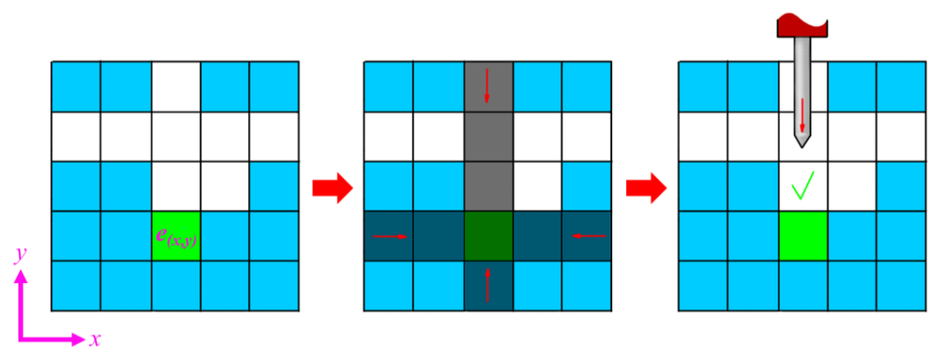
This division allows for a more detailed understanding of the machinability characteristics of the elements within the FL, providing insights into their accessibility for machining operations. For the FL elements in groups 1 and 2, the process for identifying them is as follows:
For an element to be considered directly accessible for a tool, it must satisfy a specific condition: at its free faces, there must be a row of elements with densities below the selected threshold that extends to the boundaries of the design domain. To illustrate this process, let’s consider the simplified 2D example in Error! Reference source not found., where the identification process is depicted. The blue elements represent those with densities exceeding the threshold, while the green element e(x,y) is the element currently being analyzed.
Figure 4. Element directly accessible for a tool detection process. In blue, solid phase; in green, the element under analysis in coordinates (x,y).
Preprints 109083 g004
To determine if an element satisfies th of being directly accessible for a tool in the y axis, the row and column leading to that element are analysed from the outside towards the inside in both directions (shaded elements in the central draw of Error! Reference source not found.). If at any point during the analysis an element is encountered with a density exceeding the threshold, the condition isn’t fulfilled for that specific element.
To be considered machinable through its neighbor, an element must meet a specific condition: a free row must extend to its free face. To determine this, the neighboring rows are analyzed from the outside towards the inside until reaching the free face of the element. If, during this analysis, none of the studied lines contains an element with a density above the threshold, then the condition is fulfilled, indicating that the element can be machined through its neighboring elements. Error! Reference source not found. illustrates this process in a similar manner to the explained process in Error! Reference source not found. but in the x axis direction.
Figure 5. Element accessible for a tool through a neighbor detection process. In blue, solid phase; in green, the element under analysis in coordinates (x,y).
Preprints 109083 g005
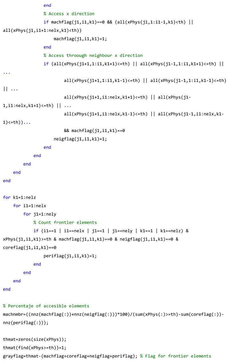
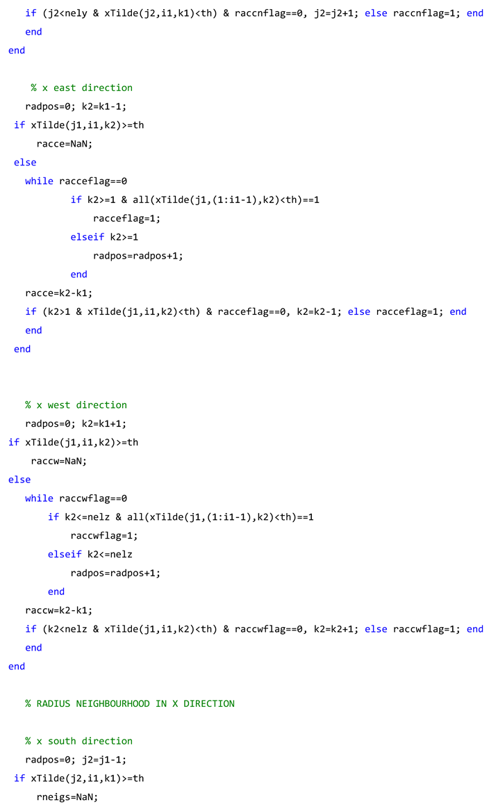
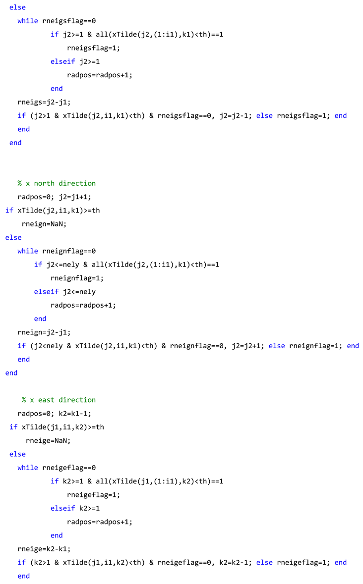
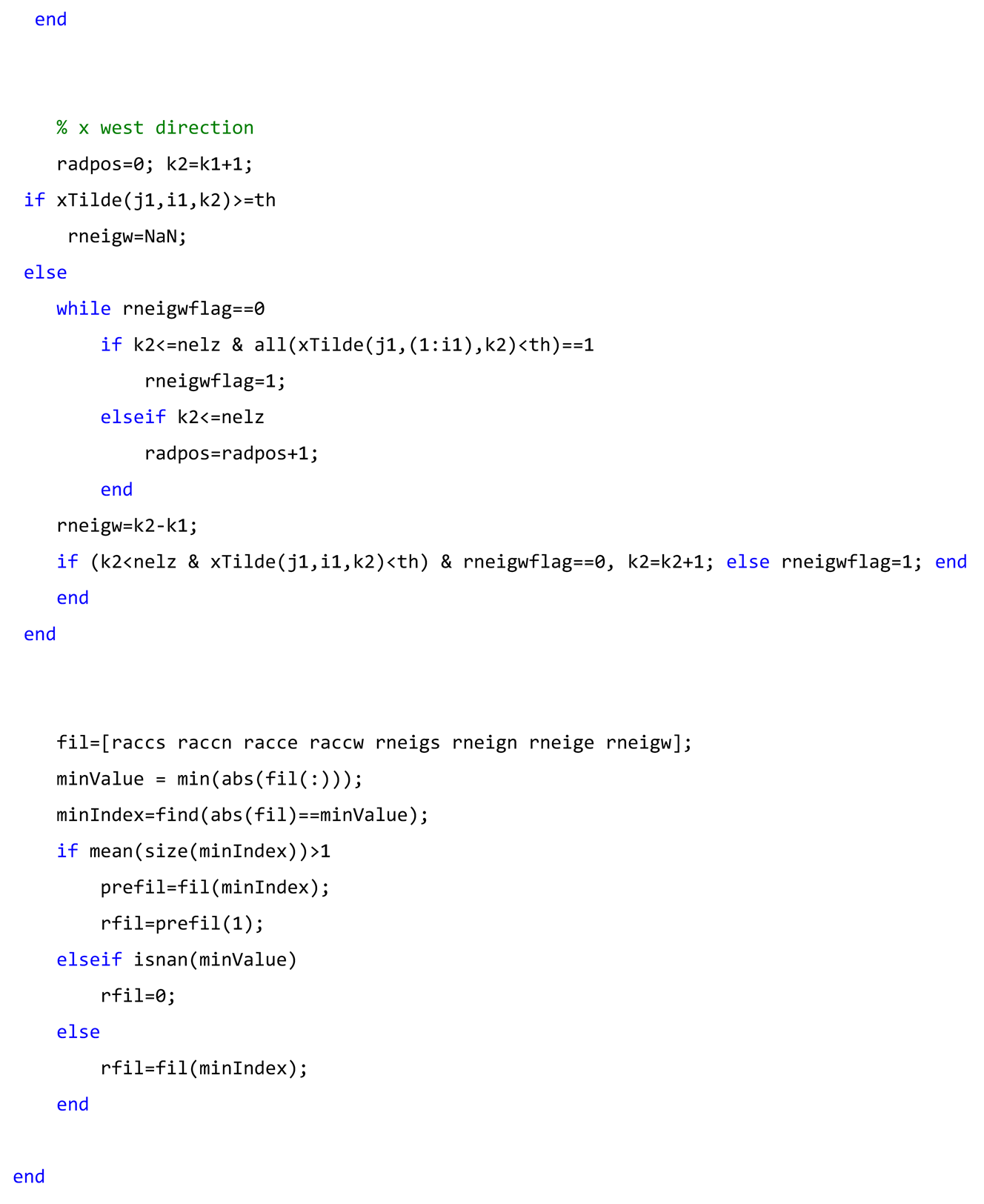
The output parameter is a percentage of the machinable elements with respect to all the frontier elements. The MATLAB ® code of this process and the rest of the machining filter (that is explained in subsequent epigraphs) are shown in Appendix A.
1. 
Sensitivity Analysis
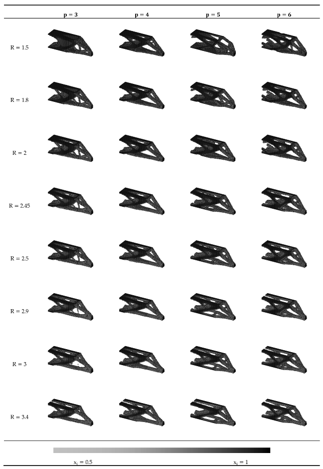
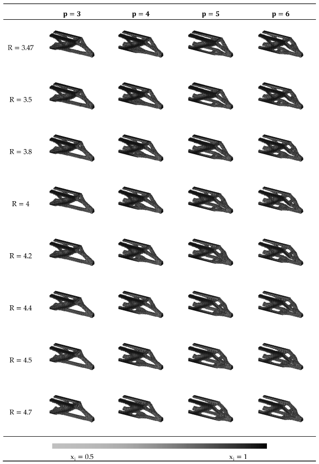
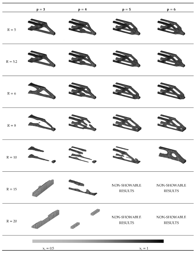
The results of the TOs are presented in Tables 1 to 4, which can be found in the Appendix B.1, Appendix B.2, Appendix B.3 and Appendix B.4. Note that the relative density x i of each element is represented with a greyscale factor in Tables 2 to 4; where a darker element represents a value closer to 1. Only elements with a relative density x i > 0.5 are shown. Finally, only full parts are considered, meaning that partial shapes with poor density concentration areas are discarded as satisfactory outcomes.
  • Numerical results for the analysis are shown in Table 1, being:
  • Sim. ID, the identifier of the specific TO case.
  • Penalization, p; and Filter Radius R.
  • Iterations, the number of iterations required to achieve the convergence condition. Note that a maximum of 5000 iterations was set, so if the TO reaches to this value, convergence is not reached.
  • It. Time, the average time the TO took in every iteration.
  • Objective, the compliance of the structure, calculated as in Equation (8):
c ( x ) = U T K U = e = 1 N E e x e u e T k 0 u e
where K , U and F are the global stiffness matrix and the global displacement and forces vectors, respectively; N is the total number of elements, u e is the e element displacement vector, k 0 is the element stiffness matrix and x e is the e element density. It is calculated in the step 3 of Error! Reference source not found., the FEM analysis. It is used as a reference value for comparing different cases.
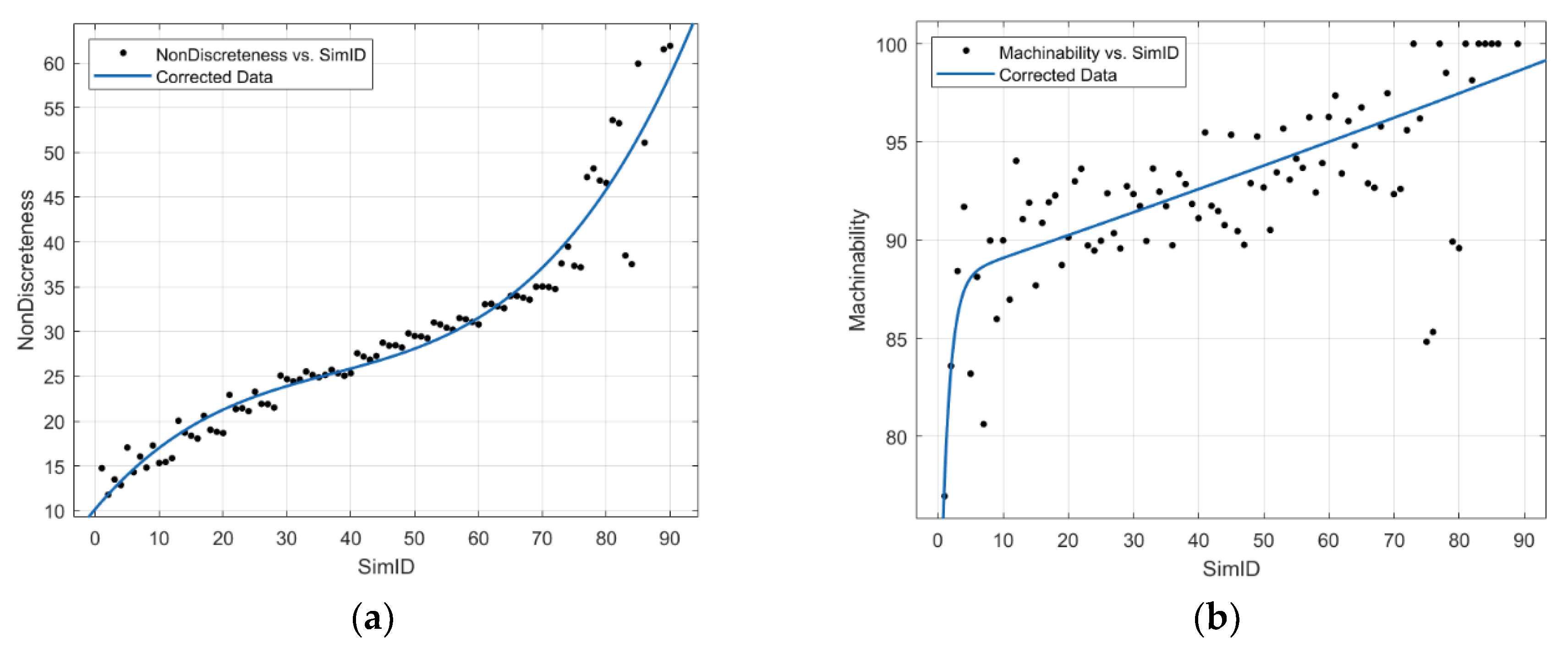
Next, in Error! Reference source not found. and Error! Reference source not found., some remarkable results are displayed along with a corrected graph of the discrete results data. The curve fitting strategy employed is a two-term exponential curve for Figure 6a, 6b and Figure 7a; and a three-term polynomial curve for Figure 7a.
As the filter radius increases, it is expected that higher filter radius values lead to simpler shapes, as the density filter in Equation (2) affects a greater number of elements. However, when the value of the radius becomes very large, the results start to exhibit discontinuities, and the computational cost increases.
Nevertheless, the corrected data depicted in Error! Reference source not found. reveals an unexpected trend. It shows that as the filter radius grows, the topology optimization (TO) process requires fewer iterations and less time per iteration for computation. This finding contradicts the initial expectation, as a larger filter radius entails analyzing more elements in each iteration.
Error! Reference source not found. provides an analysis of the manufacturability of the TOs. In Figure 7a, it is evident that higher penalization values lead to slightly lower Mnd. This is an expected outcome since higher penalization corresponds to a more aggressive interpolation of the SIMP function defined by Equation (1) and Error! Reference source not found..
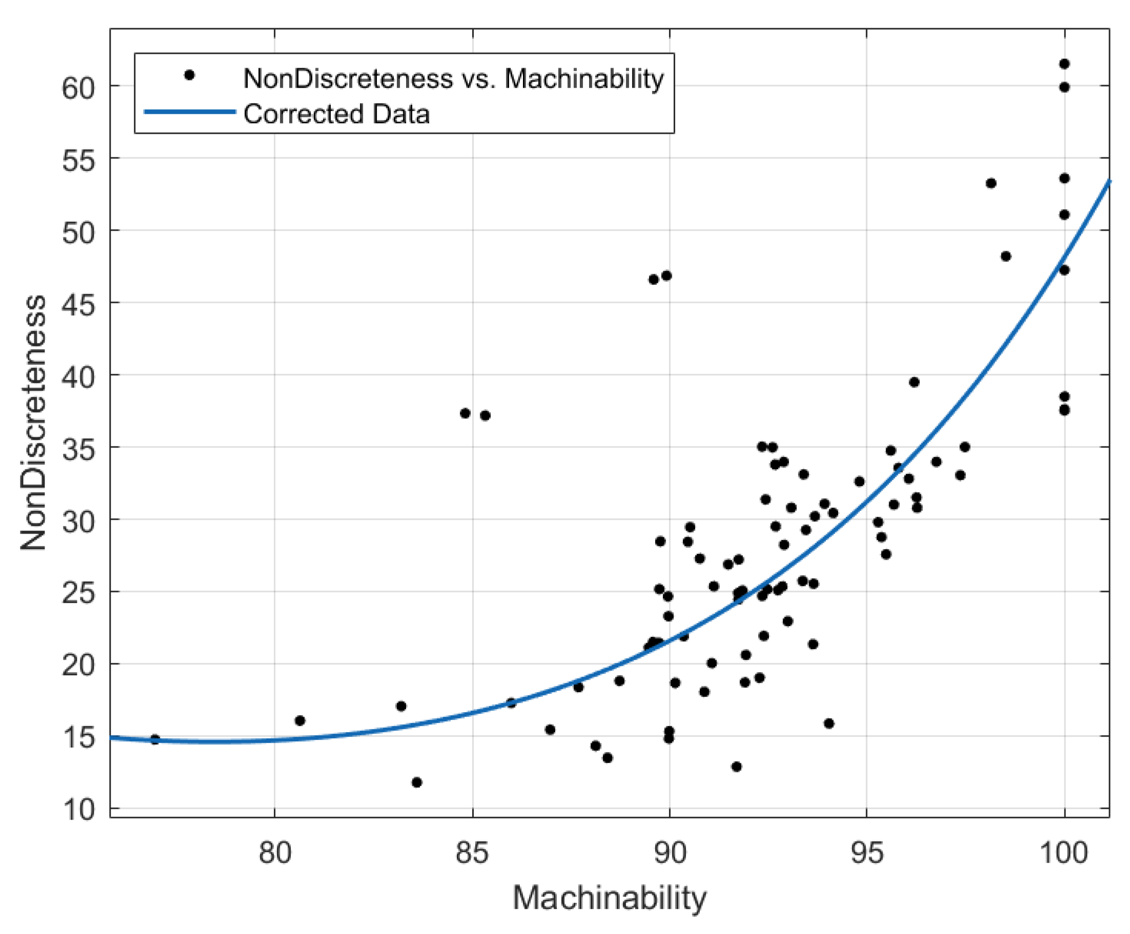
Regarding non-discreteness, the results exhibit regular and predictable behavior for filter radii ranging from 4.25% to 6.5% of the EMD (Sim. ID 19-72), and the values increase with the corresponding radii. Similarly, machinability also increases with the filter radius since, as previously mentioned, a higher radius corresponds to simpler shapes that are more easily machinable.
In Figure 7, it is observed that results become more inconsistent and exhibit greater dispersion and poor predictability when large filter radii are used. Notably, in the default density-based TO approach, it is intriguing to note that achieving the best values for discreteness and machinability simultaneously is not possible, as depicted in Figure 8. The corrected data in Figure 8 is represented using a two-term exponential curve.
Machinability filter in combination with a Heaviside step filter [16,29,30,31] may result in an improvement of the M n d -Machinability combination, as will be exposed in the next epigraph.
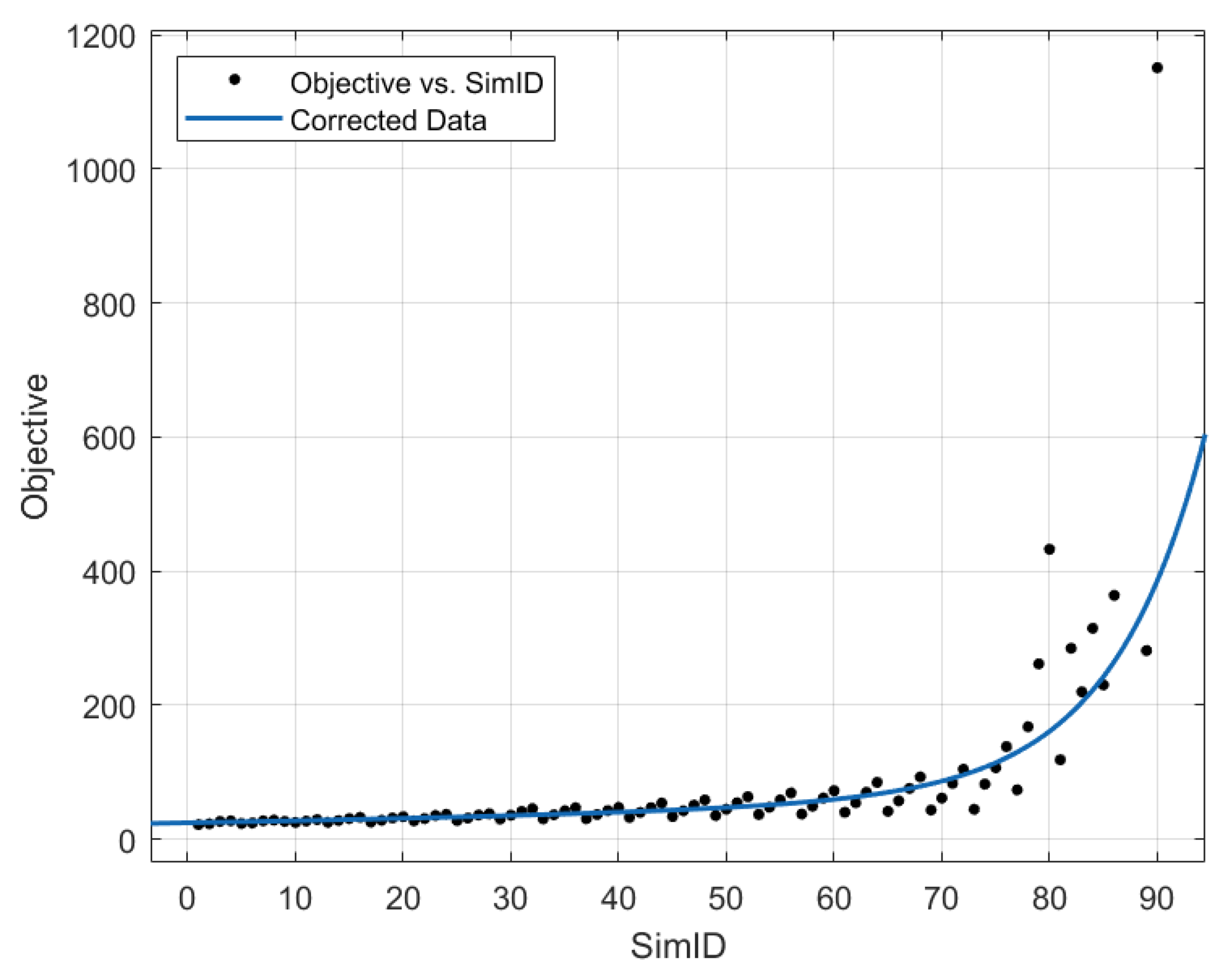
Lower filter radius and lower penalization values lead to better compliance outcomes. Additionally, results show lower dispersion with the smallest radii. These findings are expected because more complex shapes result in higher moment of inertia, leading to increased stiffness. This can clearly be seen in Figure 9, where the corrected data is represented using a two-term exponential line.
2. 
Additions to Filtering
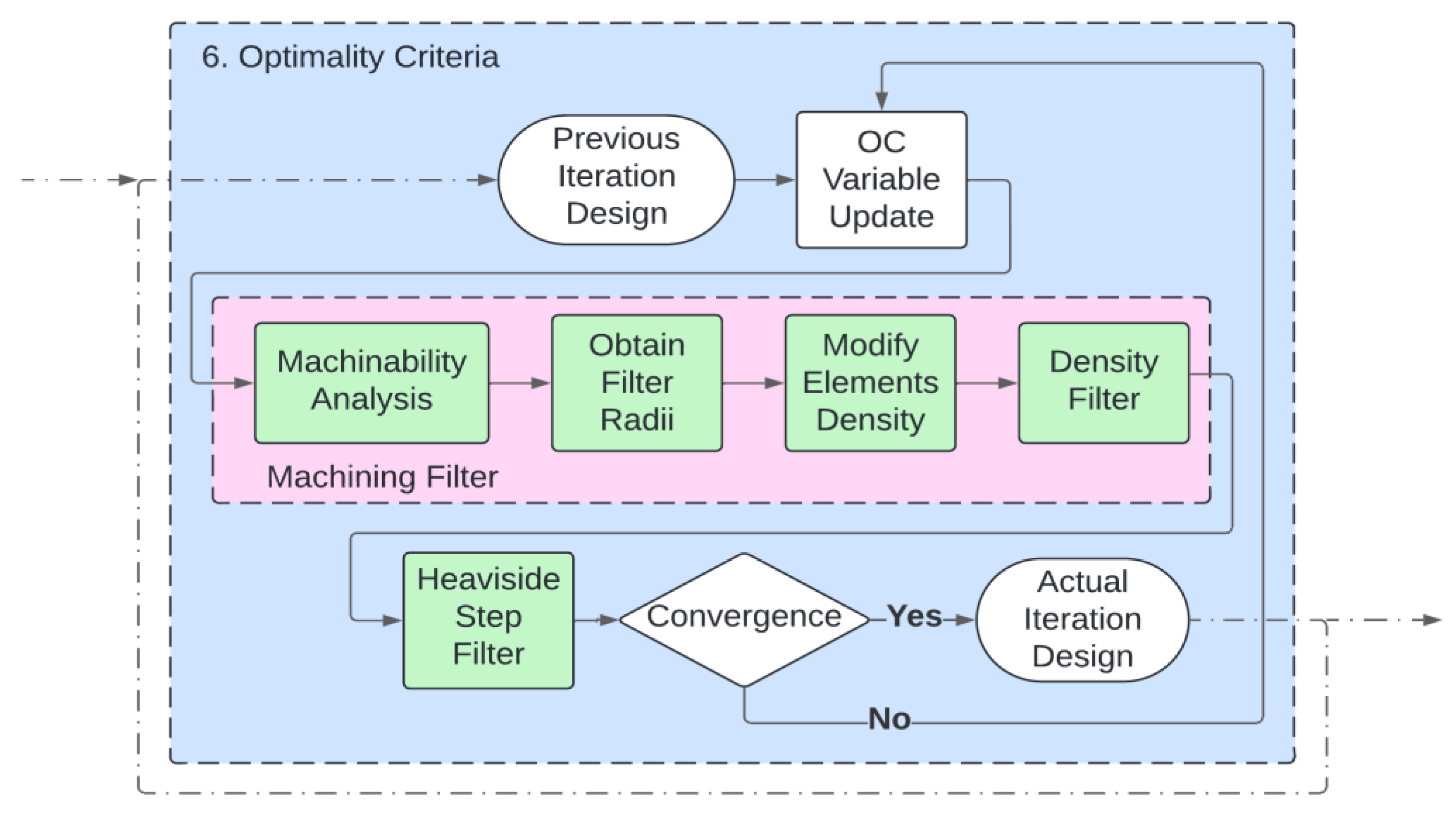
The filter is positioned inside the optimization algorithm, that in this case is the Optimality Criteria (OC) method described by Liu and Tovar in their work [6], using the parameters described in previous studies [32,33,34,35]. The flowchart depicted in Error! Reference source not found. illustrates the position of the filters (machining filter and Heaviside step filter) using the numbering notation from Error! Reference source not found..
Figure 10. Flowchart of the TO method with the machining filter highlighted in pink for clarity in later explanations.
Preprints 109083 g010
Three additions are done to the code: the machining filter, the Heaviside step filter, and the ellipsoid-shaped density filter. These implementations are next explained and positioned inside the OC routine.

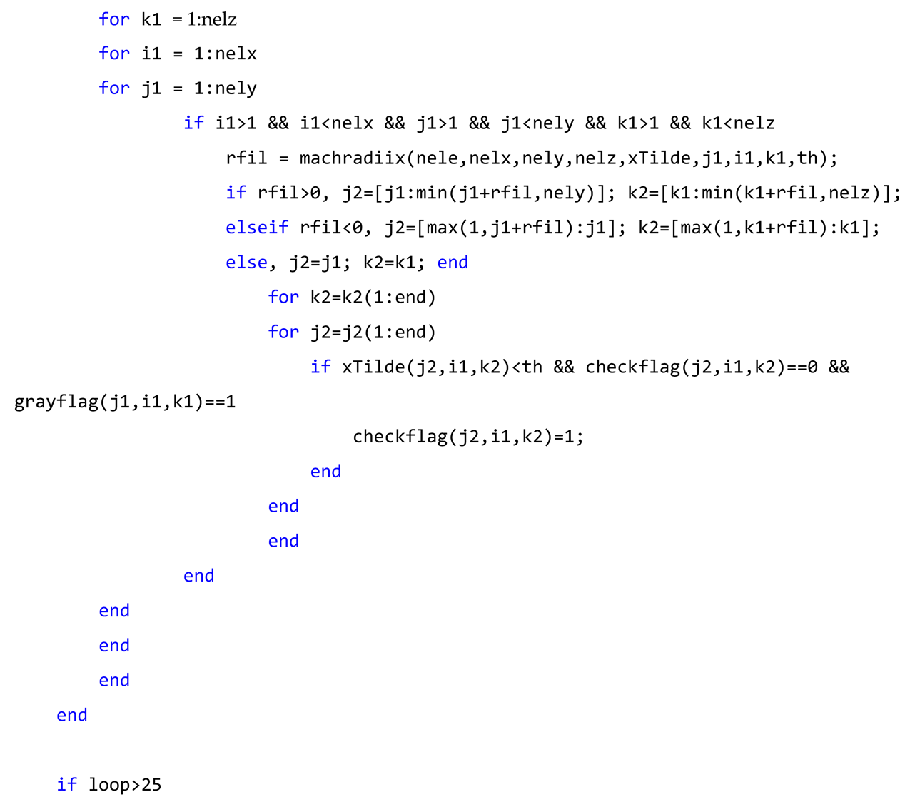
2.4. Machining Filter

The new machining filter developed for this study utilizes a method described in Section 2.3.2 to identify elements. Non-machinable elements are identified, and an individual machinability radius, Rmach, is assigned to each of them. The determination of Rmach involves analyzing the neighboring elements of the element under analysis, using the filter radii, R, described in Equation (4) and Table 1. This process is done individually for each cartesian axes, so the designer can obtain machinable parts in a concrete direction,
The analysis begins with the smallest practical radius of 1.5. If a neighboring element is deemed machinable through direct access or neighbor access, this radius is adopted, and the elements influenced by this radius are not analyzed further until the next iteration for computational efficiency. If there are no machinable elements within the neighborhood defined by the radius, the next radius in Table 1 is examined, and this process continues until at least one machinable element is found. This process MATLAB ® code is shown in Appendix B and Appendix C.
Once the non-machinable elements are detected as explained in the epigraph 0, and the filter radii are obtained, the filtering process can begin. It is graphically described in Error! Reference source not found., and it is also broken down step-by-step next.
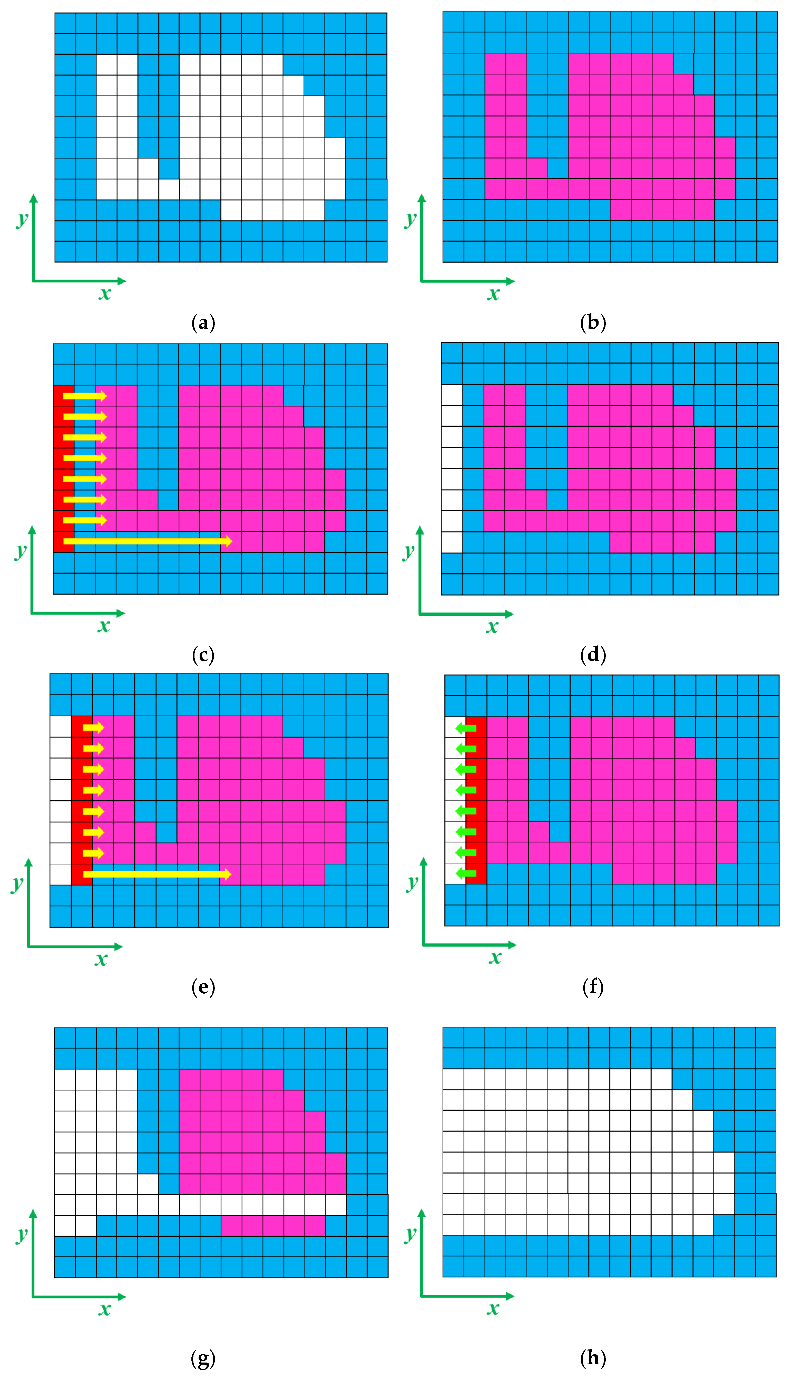
The process starts with the blueprint design, which is the resultant density field of the design variables update in the OC loop. This is represented in Figure 11a, where blue elements are the elements with a density over the chosen threshold. Then the filter radii are obtained using the MATLAB ® code of the Appendix A considering that, in this case, a machinable result in the x direction is desired. Elements highlighted in pink in Figure 11b are the ones affected by the filter radii.
Now, two conditions are evaluated: the element density (and if this density is above the density threshold) and the existence of pink elements in the machining direction at any point of the density field. If it exists an element that meets both conditions, its density is turned into zero. This is done for giving a first access to the filter for working as will be now described. This first column filtering is represented in Figure 11c, where elements in red are the elements that meet the mentioned conditions and the yellow arrows point the pink elements in the machining direction; and Figure 11d, where the design after the first column filtering is represented.
The rest of the columns are filtered in a similar way: the elements to filter are selected if they meet the conditions described above, but in this case, they take the density of the element before them in the machine direction, the (x-1,y) element. In Figure 11e, the second column element detection is represented in a similar way as in Figure 11c; and in Figure 11f, green arrows represent the elements from whom the filtered elements are taking their new density.
Figure 11g represents the density field after the second column filtering. The process continues until there’s no elements that meet the filtering conditions. In Figure 11h the final design after all the filtering process is represented. The MATLAB ® code of the filter itself is sown in Appendix C.
Finally, a kernel filter as the described in Equation 2 is applied as damping tool. Enforce some elements to have a concrete density can derive on a disintegrated density field and thus in a difficult convergence of the OC routine. This acts as the density filter [19,36] presented in Section 1 and it’s also where the ellipsoid-shaped filter is added (epigraph 4.3).

2.5. Heaviside Step Filter

To achieve a manufacturable part with minimal discretization of the element densities, a chain rule consisting of close filters through a Heaviside function as the one described by Schevens (2016), Andreassen (2007) and Pellens (2019), is used first applying a dilatation, and lastly an erosion step. Sigmund [28] demonstrated the use of close filters for reducing the discreteness of the result while preserving the original shape (non-filtered shape). The utilized Heaviside Step function corresponds to the smooth approximation proposed by Wang (2011):
ρ ¯ e = tanh β η + t a n h ( β ρ ~ e η ) tanh β η + t a n h ( β 1 η )
where β corresponds to the Heaviside smoothness parameter: a β approaching zero filters the densities linearly without making any changes, while β trending to infinite causes a step function in the value defined by the parameter η . When η = 1 , the expression corresponds to an erosion filter, while when η = 0 , it corresponds to a dilation filter. The aim of using first a dilation filter and later an eroding filter is to avoid a non-volume preserving strategy.
The sensitivities must be modified to ensure accurate calculation of the new design variables in every OC iteration. This is done through the chain rule described in Equation (10):
c x = c x ¯ x ¯ x ˇ ¯ x ˇ ¯ x ˇ ¯ ^ x ˇ ¯ ^ x ˇ ¯ ^ ^

2.6. Ellipsoid-Shaped Density Filter

The main issue when extrapoling results from the sensitivity analysis to other design spaces is the mesh dependency of the density-based TO [17]. As the shape of the optimized part is directly dependant on the density filter described in Equation (2). This is caused by the relation of the filter size and the design domain size: using the same filter size with different design domains leads to different resultant shapes.
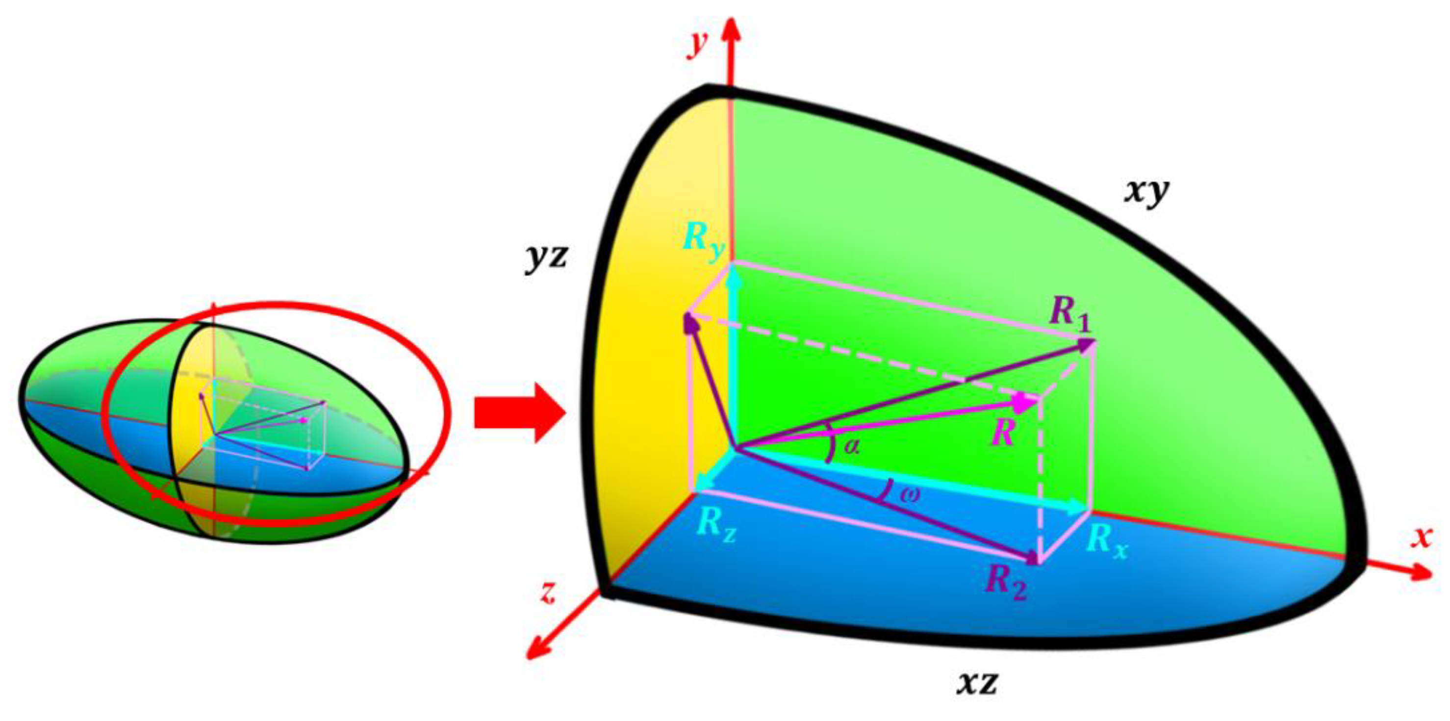
To adress this characteristic, the original sphere-shaped filter is taken as an ellipsoid with equal semi-axes, so they can be individually varied with the three cartesian dimmensions of the initial design domain. As the used weighting factor is conic weights [36], the radius of the ellipsoid at the same latitude and longitude than the analyzed element, R i j k f i l , must be obtained for calculating the weight of the neighbor elements.
For obtaining this radius, six initial parameters are needed: a , b and c , which are the semi-axes dimmensions given by the user as three filter radii R x m i n , R y m i n and R z m i n respectively; and the relative coordinates of the element being analysed in the Kernel filter with respect to the base element: R i , R j and R k .
The angles α and ω in Error! Reference source not found. are the geocentric latitude and longitude respectively, they can be obtained with trigonometry, being:
α = tan 1 R y / R x ω = tan 1 R z / R x
The coordinates of the ellipsoid surface at the same latitude and longitude than the analysed element, R x , R y and R z , can be geometrically calculated. Combining these values with the general formula of an ellipsoid, Equation (12) is obtained for the calculation of the desired radius:
R i j k f i l = a b c c 2 cos 2 ( ω ) b 2 cos 2 α + a 2 s e n 2 ( α ) + a 2 b 2 cos 2 α s e n 2 ( ω )
The three implementations are presented and highlighted in green in the flowchart presented in Error! Reference source not found.. The flowchart represents the level 6 of the Error! Reference source not found. and the blue block of the Error! Reference source not found.. The machining filter is divided into the three phases described in Appendix A.1, Appendix A.2 and Appendix A.3; and both density filters are computed with the ellipsoid-shaped neighborhood.
Figure 13. OC routine with the machining filter highlighted in pink and the colored in green.
Preprints 109083 g013

3. Results

This section is divided in two parts. The first one is a validation of the proposed additions to the original TO methodology. In this subsection a concrete case of the sensitivity analysis is chosen, and the machining filter, the ellipsoid-shaped density filter and the Heaviside step filter are applied separately and at once to show the impact in the results and verify their performance. The second subsection is an epigraph explaining the conclusions reached in this study, highlighting the most useful points for the potential designers that read this paper.

3.1. Validation

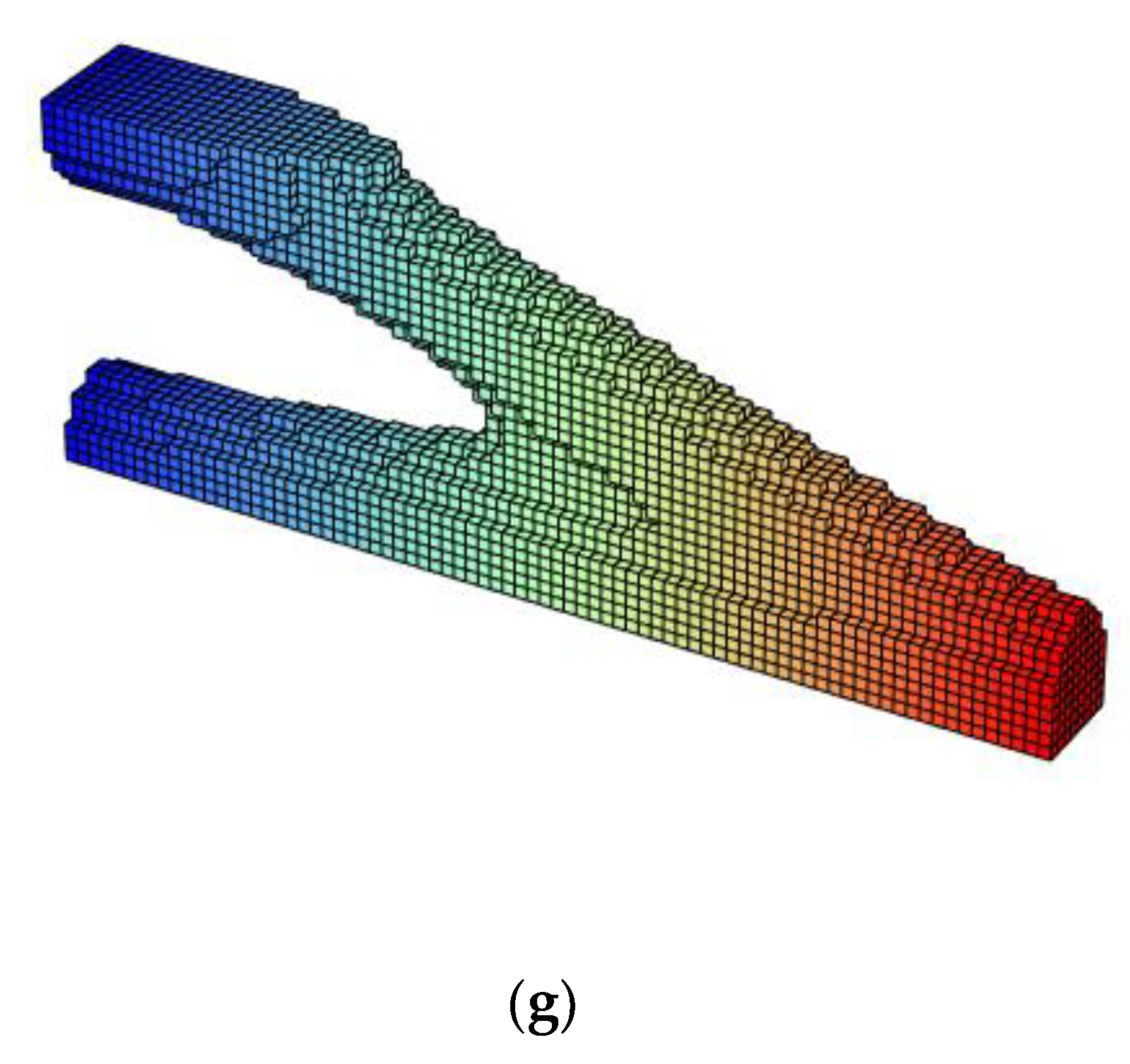
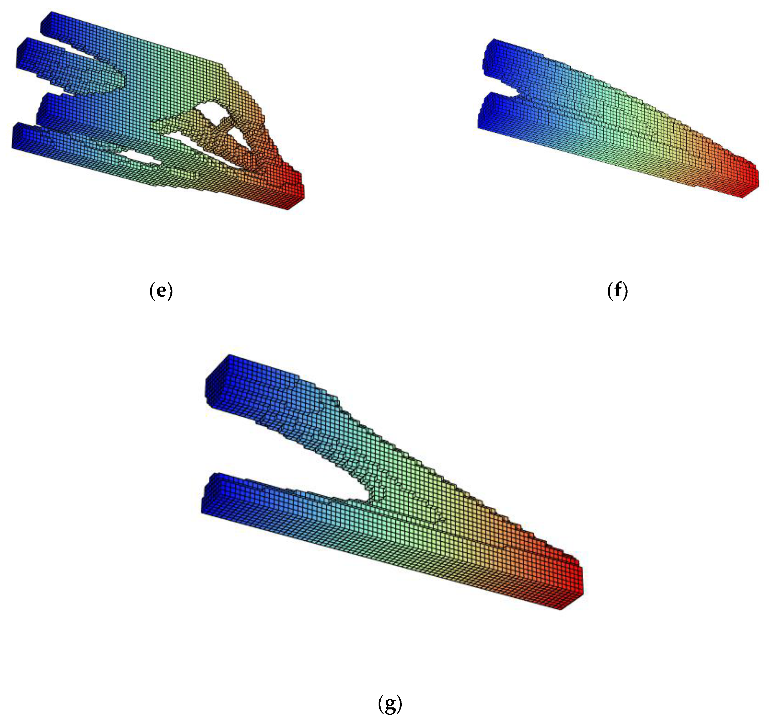
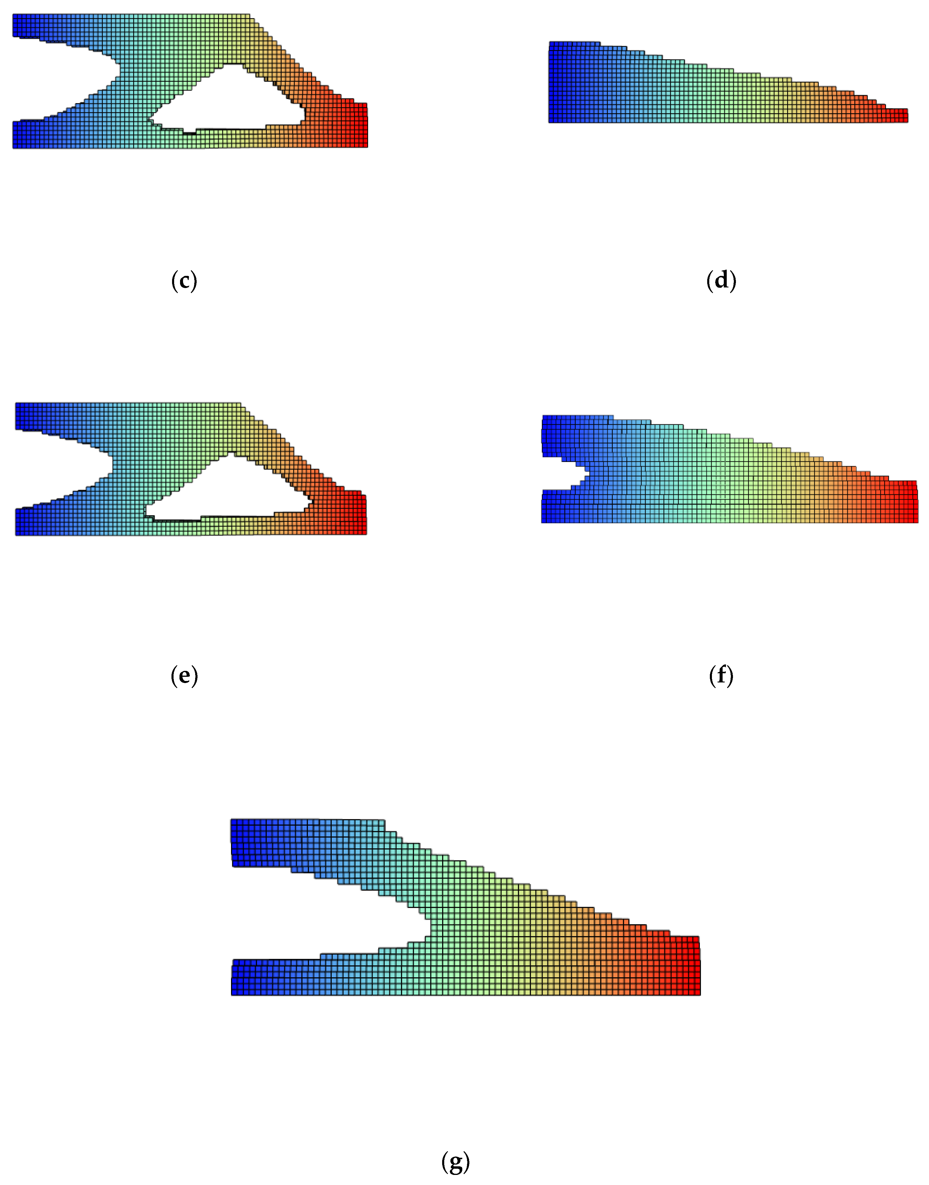
In this subsection, six different validation cases are analyzed based on the subcase R = 3 and p = 6 , whose data and shape can be seen in Appendix B.1 and Appendix B.2. All the figures are colored rainbow-like in the machining direction, starting in blue and finishing in red. This is done for having a clearer view of the results and the difference between the resultant shapes of the validation cases.
For the cases (c), (d), (e) and (f), that are the cases where the Heaviside filter is applied, the searching methodology described in [37] is applied, updating the design variables every 25 iterations or when the updating conditions are met. Finally, a case (g) is showcased where the number of iterations for updating the design variables is reduced to 10 with the conditions of case (f) for reducing the total number of iterations and search for an optional different design. A video showcasing case (g) and the AVD described in [37] is available in the Data Availability Statement section.
Relevant data of the validation are presented in Table 2, where the number of iterations before convergence, the measure of non-discreteness, the machinability and the compliance (as objective function) of all the verification cases are showed.

3.2. Conclusions

Through this study, several conclusions can be drawn regarding the parameters to be considered for designers when using TO as design methodology, as well as how to fix the issues found. The proposed solutions can be interpreted as potential implementations for commercial software packages in the future, as they haven’t implemented this kind of methodologies yet.
In the sensitivity analysis, modification over the penalization and filter radius are analyzed in a concrete 3D case. 92 simulations are showcased, being the most complete study of this kind found in the bibliography. The results are commented in Section 3, but here some notes are added regarding the aim of the paper: helping designers. The interesting thing in a TO when designing functional parts is having a low interpretation of the optimized shape (this is low M n d ), high machinability and the lower objective function as possible for the prescribed constraints (compliance and volume fraction respectively in the case study).
The main issue detected in the sensitivity analysis is the fact that a low measure of non-discreteness M n d and high machinability can’t be achieved at the same time. This can be seen in Error! Reference source not found., but specially in Error! Reference source not found., where the described relation is evidenced with the discrete data of the results. As the volume fraction is the same for all the simulations, the objective is clearly dependant on the penalization, obtaining better results for low penalizations as Error! Reference source not found. and Appendix B.1 evidence; but worse non-discreteness results are obtained for that low penalization factors (Error! Reference source not found.). Machinability finds a trend in the filter radius, being more manufacturable the results with high value of that radius as Figure 7 shows.
Here, the necessity of additions for obtaining the best possible results in terms of interpretation and manufacturability is detected. For this paper, three additions have been studied and applied (being two of them a novelty): the machining filter, the ellipsoid-shaped density filter and the Heaviside step filter. The machining filter have been developed for obtaining machinable parts in a concrete direction; the ellipsoid-shaped density filter has the aim of obtain results with concrete features in certain selective directions (looking for example the results of the sensitivity analysis) and the Heaviside step filter is applied for obtaining low interpretation of the results or, in other words, low measure of non-discreteness.
Table 2 and Appendix C evidence the successful addition of the three filters separately and combined. In the cases where the machining filter is applied (cases (d) and (f)), a machinability of 100% is achieved with a higher computation cost (more iterations until convergence and more time per iteration). The cases where Heaviside step filter is used (cases (b), (d), (e) and (f)), M n d is sensibly lower than “standard” cases. Finally, the cases where the ellipsoid-shaped density filter is applied (cases (c) and (e)), the machinability is a bit better in comparison to those cases without the filter, but the interesting thing is achieving the described desired features of different cases seen in the sensitivity analysis.
Considering this, and specially looking to cases (f) and (g), the behaviour end effectiveness of the developed filters is verified, as a low M n d is obtained while having a 100% of machinability. The incrementation of the iterations until convergence is a normal consequence of adding extra constraints (filters in this case), as well as the increase of the objective function, but modifying the AVD [37] parameters, it can get to convergence while keeping a high discreteness, a 100% machinability and low objective function compared to non-constrained designs. Geometrical restrictions introduce dramatic limitations into the possible optimum shapes, but it’s the only way to mathematically ensure that an optimum design is reached and allow the designers to use the obtained shapes with low interpretation of the results.
In summary, the sensitivity analysis carried out in this study is a good tool for designers to choose the initial parameters of their TOs, and they can be useful for getting to some geometrical features through the ellipsoid-shaped density filter. The Heaviside step filter is a valuable tool for obtaining low interpretable designs (with high discretization of the density field), ensuring a good results interpretation stage. The presented machining filter have demonstrated to be an interesting tool for obtaining machinable parts in a certain direction, and it could be a powerful tool in combination with the other additions presented in the paper. Nevbertheless, a convergence or searching strategy should be used (Adaptaive Variable Design, that have proven its effectiveness; use of other optimization algorithms or a user custom strategy, etc.).

Author Contributions

Conceptualization, A.V.; methodology, A.V., J.M. and A.B.; software, A.V..; validation A.V., J.M. and A.B.; investigation, A.V.; resources, C.C..; writing—original draft preparation, A.V., J.M. and A.B.; writing—review and editing, A.V., J.M. and A.B.; supervision, J.M. and A.B; project administration, C.C.; funding acquisition, C.C. All authors have read and agreed to the published version of the manuscript.

Funding

The research work described in this paper is part of the R&D and Innovation projects MC4.0 PID2020-116984RB-C21 and MC4.0 PID2020-116984RB-C22 supported by the MCIN/AEI/10.13039/501100011033

Data Availability Statement

The original data presented in the study are openly available the appendices section of this paper. Further questions about the implementation, understanding and use of the data can be submitted to the corresponding author. A video of the case (g) has been generated and is available in the next Dropbox link: https://www.dropbox.com/scl/fi/oxgbuo7mamzugsgxqe7m5/Case-g.avi?rlkey=ocer0yqjskmoxidv2sf6hu0ey&st=sbuxk78y&dl=0

Acknowledgments

The research work described in this paper is part of the R&D and Innovation projects MC4.0 PID2020-116984RB-C21 and MC4.0 PID2020-116984RB-C22 supported by the MCIN/AEI/10.13039/501100011033. Authors specially thank the Department of Industrial Engineering of the Alma Mater Studiorum Università di Bologna and their research group for allowing the collaboration and stay in their campus.

Conflicts of Interest

The authors declare no conflicts of interest.

Appendix A

Appendix A.1. Machinability MATLAB ® Code
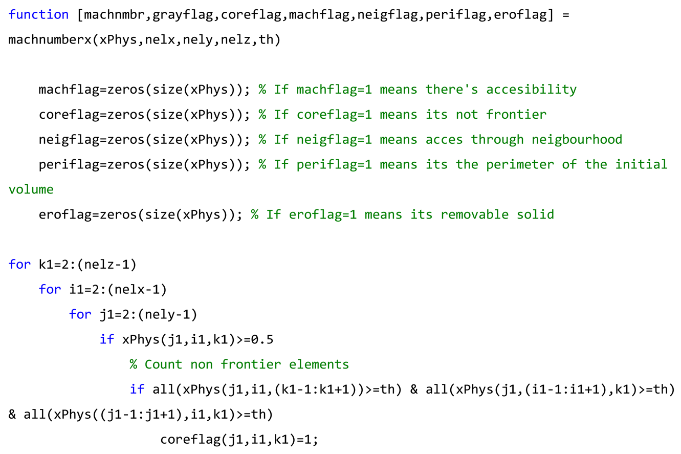
Preprints 109083 i004Preprints 109083 i005Preprints 109083 i006

Appendix A.2. Filter Radii MATLAB ® Code
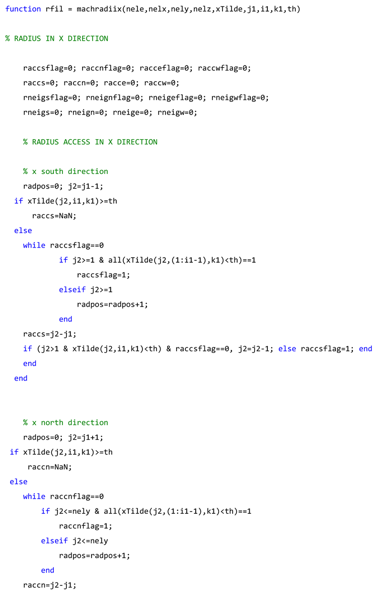
Preprints 109083 i007Preprints 109083 i008Preprints 109083 i009Preprints 109083 i010

Appendix A.3. Machining Filter MATLAB ® Code
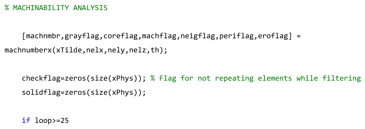
Preprints 109083 i011Preprints 109083 i012

Appendix B

Appendix B.1. Numerical Results of the Sentitivity Analysis

Sim. ID Penalization Filter Radius Iterations It. Time
[s]
Objective Non-Discreteness Machinability
1 3 1,5 567 13,884 21,943 14,744 76,959
2 4 1,5 816 11,939 23,102 11,78 83,592
3 5 1,5 1677 11,938 26,6456 13,481 88,424
4 6 1,5 1122 11,919 27,5479 12,866 91,694
5 3 1,8 820 11,656 23,545 17,052 83,195
6 4 1,8 714 11,851 24,3423 14,309 88,123
7 5 1,8 765 11,813 27,4922 16,05 80,631
8 6 1,8 777 11,387 28,5529 14,818 89,976
9 3 2 1122 11,944 26,6273 17,28 85,983
10 4 2 624 11,229 25,0757 15,325 89,987
11 5 2 1048 11,618 27,2029 15,431 86,971
12 6 2 750 14,152 29,3505 15,861 94,034
13 3 2,45 1043 10,221 25,2856 20,039 91,066
14 4 2,45 845 9,914 27,9992 18,703 91,904
15 5 2,45 953 11,012 30,9835 18,375 87,688
16 6 2,45 1336 10,713 32,7265 18,054 90,878
17 3 2,5 1009 10,158 25,6883 20,603 91,927
18 4 2,5 1345 10,036 28,412 19,025 92,277
19 5 2,5 1338 11,255 31,8068 18,811 88,728
20 6 2,5 1253 11,784 33,5945 18,666 90,139
Sim. ID Penalization Filter Radius Iterations It. Time
[s]
Objective Non-Discreteness Machinability
21 3 2,9 989 10,025 27,5435 22,934 92,992
22 4 2,9 1212 10,278 30,833 21,347 93,632
23 5 2,9 1224 10,549 35,4921 21,445 89,727
24 6 2,9 1082 11,362 37,2027 21,114 89,466
25 3 3 752 10,991 27,9193 23,285 89,966
26 4 3 1017 10,241 31,6539 21,926 92,385
27 5 3 1003 10,203 36,2139 21,896 90,352
28 6 3 1018 10,88 38,0111 21,506 89,577
29 3 3,4 628 10,129 30,2176 25,09 92,742
30 4 3,4 1089 10,766 35,8477 24,691 92,343
31 5 3,4 752 10,997 41,52 24,442 91,737
32 6 3,4 449 11,209 45,7168 24,655 89,955
33 3 3,47 1232 10,237 30,586 25,537 93,644
34 4 3,47 979 10,822 36,5405 25,151 92,466
35 5 3,47 545 9,888 42,4405 24,893 91,731
36 6 3,47 697 10,344 46,9585 25,162 89,736
37 3 3,5 1068 10,577 30,7718 25,73 93,368
38 4 3,5 890 10,576 36,8576 25,353 92,852
39 5 3,5 675 10,72 42,7654 25,069 91,84
40 6 3,5 686 10,207 47,569 25,362 91,116
Sim. ID Penalization Filter Radius Iterations It. Time
[s]
Objective Non-Discreteness Machinability
41 3 3,8 695 14,976 32,6765 27,575 95,482
42 4 3,8 704 14,976 40,071 27,215 91,743
43 5 3,8 652 9,903 47,0157 26,87 91,478
44 6 3,8 817 11,018 54,1068 27,279 90,762
45 3 4 836 10,748 34,034 28,765 95,363
46 4 4 614 11,769 42,5076 28,438 90,458
47 5 4 626 10,367 50,9945 28,469 89,762
48 6 4 584 9,966 58,6735 28,232 92,896
49 3 4,2 617 12,87 35,3255 29,798 95,279
50 4 4,2 743 10 44,8544 29,507 92,683
51 5 4,2 915 12,313 54,5237 29,452 90,514
52 6 4,2 934 10,778 63,434 29,257 93,449
53 3 4,4 647 10,607 36,9453 31,019 95,679
54 4 4,4 501 10,435 47,8507 30,796 93,079
55 5 4,4 744 10,185 58,8192 30,438 94,141
56 6 4,4 736 9,681 69,2076 30,209 93,676
57 3 4,5 1149 9,686 37,6527 31,513 96,252
58 4 4,5 415 10,5277 49,3779 31,372 92,43
59 5 4,5 422 10,185 61,3949 31,067 93,922
60 6 4,5 580 9,973 72,4609 30,8 96,268
Sim. ID Penalization Filter Radius Iterations It. Time
[s]
Objective Non-Discreteness Machinability
61 3 4,8 1019 10,463 40,1734 33,049 97,36
62 4 4,8 573 10,778 54,4644 33,106 93,393
63 5 4,8 699 10,476 70,182 32,808 96,059
64 6 4,8 528 10,727 84,8949 32,616 94,806
65 3 5 810 9,537 41,7655 33,98 96,755
66 4 5 907 9,736 57,4949 33,979 92,887
67 5 5 851 10,553 75,8592 33,789 92,671
68 6 5 606 11,068 93,0405 33,562 95,795
69 3 5,2 779 9,313 43,6644 35,008 97,477
70 4 5,2 1091 9,651 61,3489 35,032 92,34
71 5 5,2 1051 9,884 83,3058 34,979 92,605
72 6 5,2 337 9,899 104,346 34,754 95,6
73 3 6 535 9,224 44,6408 37,613 100
74 4 6 505 9,413 82,3081 39,494 96,195
75 5 6 1149 10,701 106,722 37,338 84,818
76 6 6 1015 10,892 138,359 37,181 85,325
77 3 8 473 9,941 73,6699 47,258 100
78 4 8 396 10,078 167,952 48,21 98,516
79 5 8 452 10,246 261,633 46,87 89,919
80 6 8 576 10,743 432,583 46,606 89,592
Sim. ID Penalization Filter Radius Iterations It. Time
[s]
Objective Non-Discreteness Machinability
81 3 10 381 10,982 118,666 53,618 100
82 4 10 1144 13,666 284,998 53,272 98,14
83 5 10 1811 14,05 219,921 38,502 100
84 6 10 3986 17,087 314,672 37,534 100
85 3 15 238 19,017 230,282 59,919 100
86 4 15 1083 20,813 363,853 51,092 100
87 5 15 5000 NaN NaN NaN NaN
88 6 15 5000 NaN NaN NaN NaN
89 3 20 119 30,664 281,498 61,537 100
90 4 20 189 33,328 1150,9 61,91 NaN
91 5 20 5000 NaN NaN NaN NaN
92 6 20 5000 NaN NaN NaN NaN

Appendix B.2. Results of the sensitivity analysis for 1.5 ≤ R ≤ 3.4
Preprints 109083 i001

Appendix B.3. Results of the Sensitivity Analysis for 3.47 ≤ R ≤ 4.7
Preprints 109083 i002

Appendix B.4. Results of the Sensitivity Analysis for 5 ≤ R ≤ 20
Preprints 109083 i003

Appendix C

Appendix C.1. Verifications: Superior Perspective View
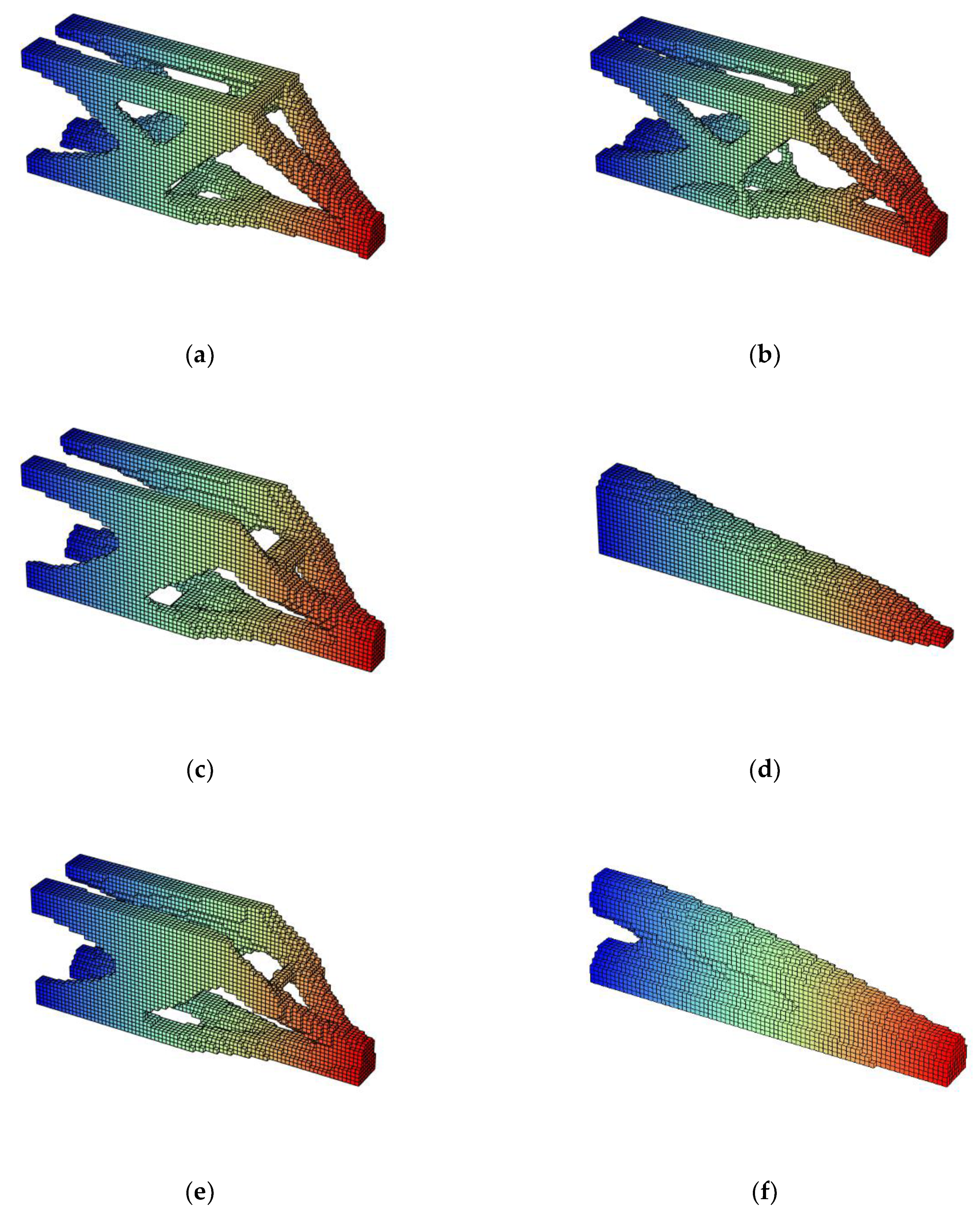
Figure A1. Superior perspective view of the different validation cases. (a) Standard case. (b) Heaviside step filter. (c) Ellipsoid-shaped filter. (d) Machining filter. (e) Ellipsoid-shaped filter + Heaviside step filter. (f) Machining filter + ellipsoid-shaped filter. (g) Machining filter + ellipsoid-shaped filter + changes in adaptive design variable method [37].
Preprints 109083 g0a1aPreprints 109083 g0a1b

Appendix C.2. Verifications: Inferior Perspective View
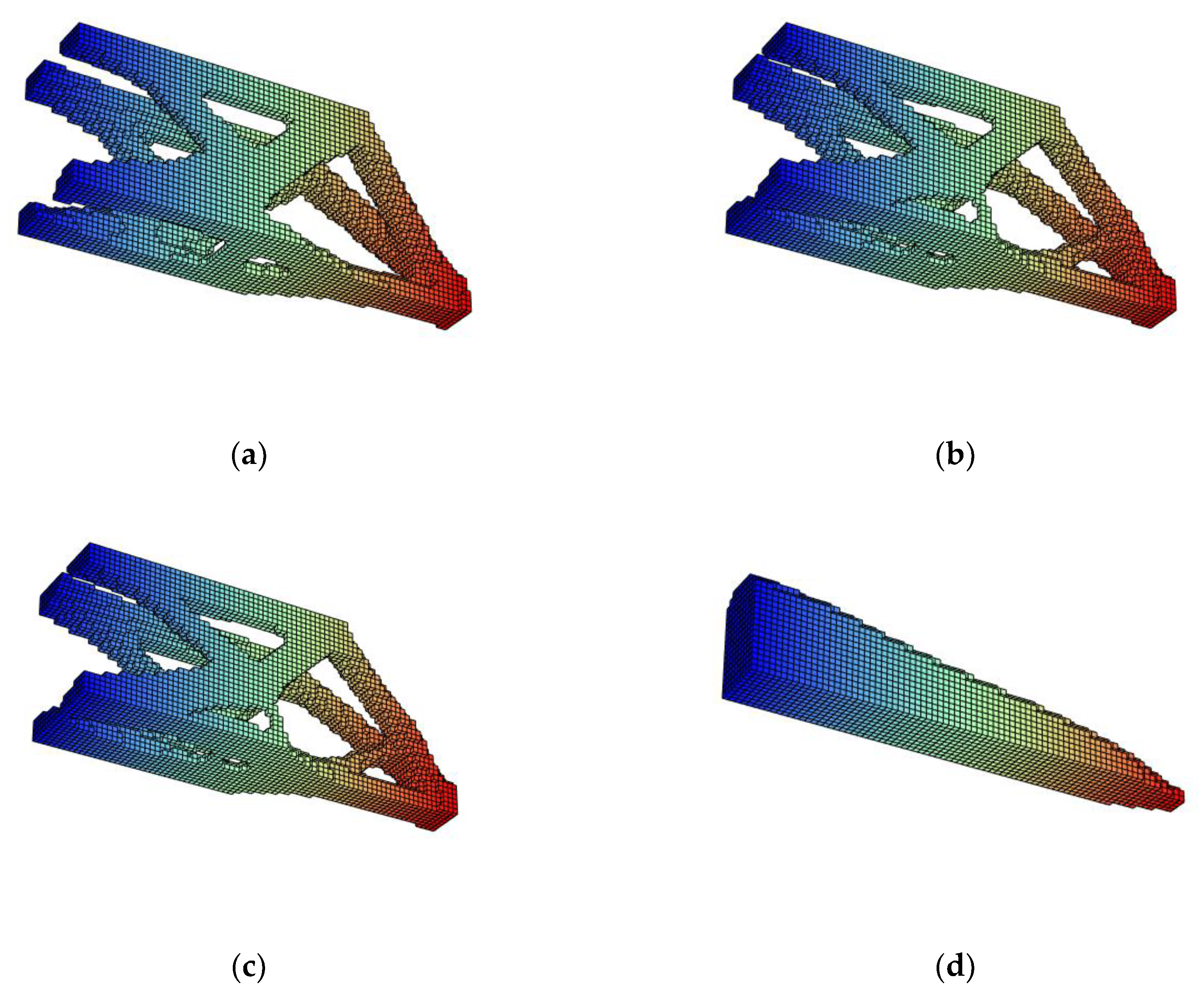
Figure A2. Inferior perspective view of the different validation cases. (a) Standard case. (b) Heaviside step filter. (c) Ellipsoid-shaped filter. (d) Machining filter. (e) Ellipsoid-shaped filter + Heaviside step filter. (f) Machining filter + ellipsoid-shaped filter. (g) Machining filter + ellipsoid-shaped filter + changes in adaptive design variable method [37].
Preprints 109083 g0a2aPreprints 109083 g0a2b

Appendix C.3. Verifications: Lateral View
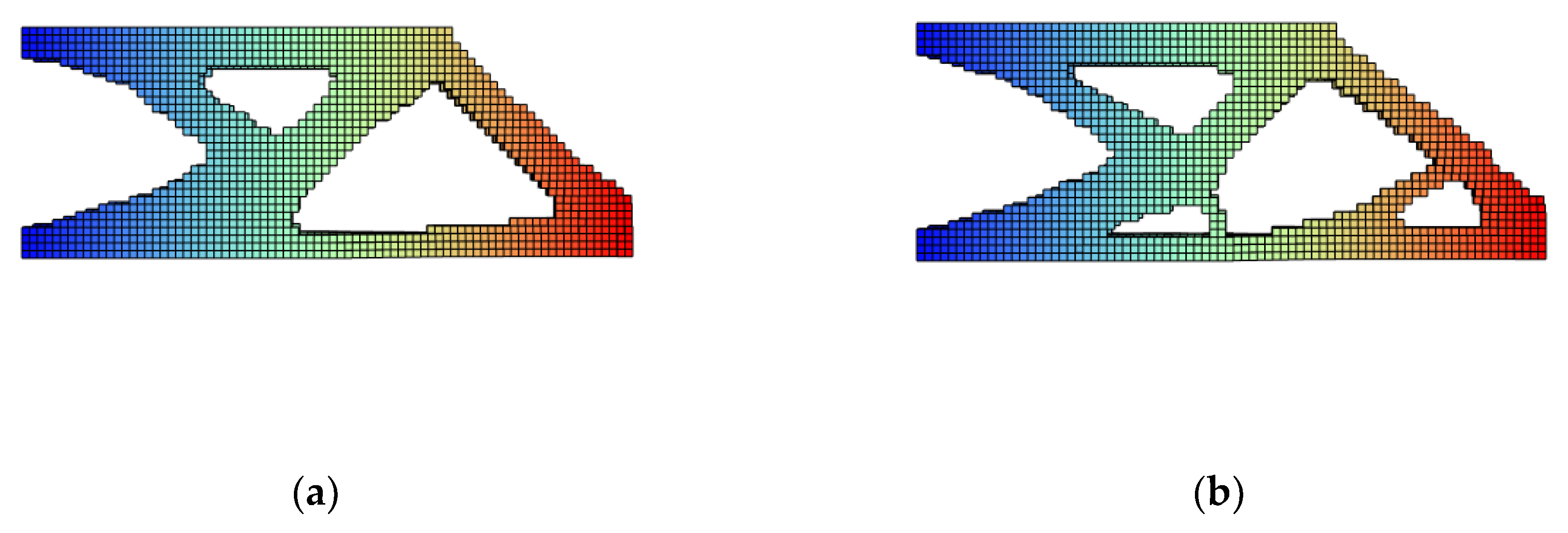
Figure A3. Lateral view of the different validation cases. (a) Standard case. (b) Heaviside step filter. (c) Ellipsoid-shaped filter. (d) Machining filter. (e) Ellipsoid-shaped filter + Heaviside step filter. (f) Machining filter + ellipsoid-shaped filter. (g) Machining filter + ellipsoid-shaped filter + changes in adaptive design variable method [37].
Preprints 109083 g0a3aPreprints 109083 g0a3b

Appendix C.4. Verifications: Front View
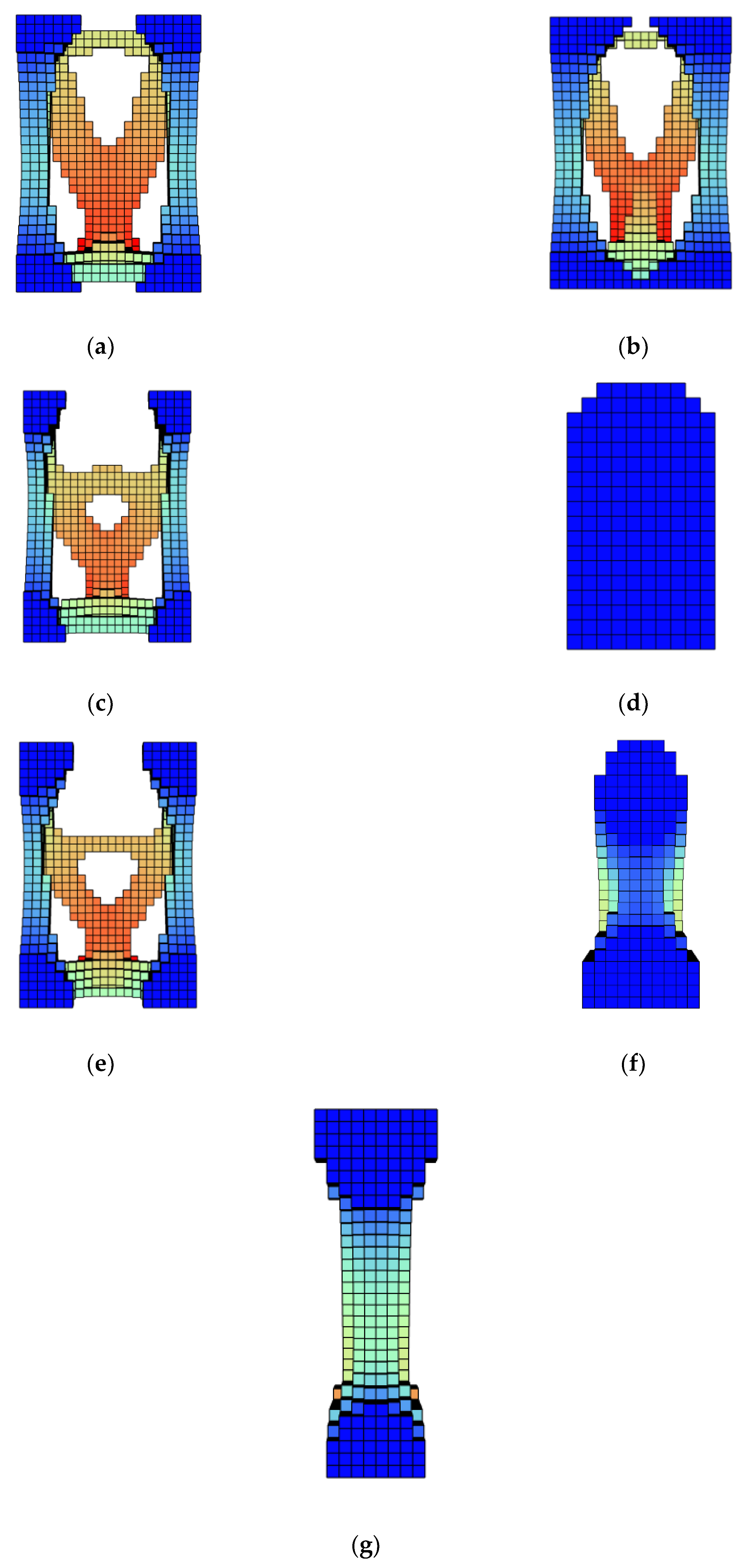
Figure A4. Front view of the different validation cases. (a) Standard case. (b) Heaviside step filter. (c) Ellipsoid-shaped filter. (d) Machining filter. (e) Ellipsoid-shaped filter + Heaviside step filter. (f) Machining filter + ellipsoid-shaped filter. (g) Machining filter + ellipsoid-shaped filter + changes in adaptive design variable method [37].
Preprints 109083 g0a4

References

  1. Shiye, B.; Jiejiang, Z. Topology Optimization Design of 3D Continuum Structure with Reserved Hole Based on Variable Density Method. Journal of Engineering Science and Technology Review 2016, 9, 121–128. [CrossRef]
  2. Michell, A.G.M. LVIII. The Limits of Economy of Material in Frame-Structures. The London, Edinburgh, and Dublin Philosophical Magazine and Journal of Science 1904, 8, 589–597. [CrossRef]
  3. Dorn, W.S.; Gomory, R.E.; Greenberg, H.J. Automatic Design of Optimal Structures. Journal de Mécanique 1964, 3.
  4. Bendsøe, M.P.; Kikuchi, N. Generating Optimal Topologies in Structural Design Using a Homogenization Method. Comput Methods Appl Mech Eng 1988, 71, 197–224. [CrossRef]
  5. Sigmund, O.; Maute, K. Topology Optimization Approaches. Structural and Multidisciplinary Optimization 2013, 48, 1031–1055. [CrossRef]
  6. Liu, K.; Tovar, A. An Efficient 3D Topology Optimization Code Written in Matlab. Structural and Multidisciplinary Optimization 2014, 50, 1175–1196. [CrossRef]
  7. Ferrari, F.; Sigmund, O. A New Generation 99 Line Matlab Code for Compliance Topology Optimization and Its Extension to 3D. Structural and Multidisciplinary Optimization 2020, 62, 2211–2228. [CrossRef]
  8. Bendsøe, M.P. Optimal Shape Design as a Material Distribution Problem. Structural Optimization 1989, 1, 193–202. [CrossRef]
  9. Mlejnek, H.P. Some Aspects of the Genesis of Structures. Structural Optimization 1992, 5, 64–69. [CrossRef]
  10. Kohn, R. V.; Strang, G. Optimal Design and Relaxation of Variational Problems, II. Commun Pure Appl Math 1986, 39, 139–182. [CrossRef]
  11. Haber, R.B.; Jog, C.S.; Bendsøe, M.P. A New Approach to Variable-Topology Shape Design Using a Constraint on Perimeter. Structural Optimization 1996, 11, 1–12. [CrossRef]
  12. Jog, C.S. A Robust Dual Algorithm for Topology Design of Structures in Discrete Variables. Int J Numer Methods Eng 2001, 50, 1607–1618. [CrossRef]
  13. Duysinx, P. Layout Optimization: A Mathematical Programming Approach; Lyngby, 1997;
  14. Bendsøe, M.P. Optimal Shape Design as a Material Distribution Problem. Structural Optimization 1989, 1, 193–202. [CrossRef]
  15. Zhou, M.; Rozvany, G.I.N. The COC Algorithm, Part II: Topological, Geometrical and Generalized Shape Optimization. Comput Methods Appl Mech Eng 1991, 89, 309–336. [CrossRef]
  16. Andreassen, E.; Clausen, A.; Schevenels, M.; Lazarov, B.S.; Sigmund, O. Efficient Topology Optimization in MATLAB Using 88 Lines of Code. Structural and Multidisciplinary Optimization 2011, 43, 1–16. [CrossRef]
  17. Tyflopoulos, E.; Flem, D.T.; Steinert, M.; Olsen, A. State of the Art of Generative Design and Topology Optimization and Potential Research Needs.; Linköping, Sweden, August 14 2018.
  18. Bendsøe, M.P.; Sigmund, O. Topology Optimization: Theory, Methods, and Applications.; 2nd ed.; Springer Science & Business Media, 2003;
  19. Bruns, T.E.; Tortorelli, D.A. Topology Optimization of Non-Linear Elastic Structures and Compliant Mechanisms. Comput Methods Appl Mech Eng 2001, 190, 3443–3459. [CrossRef]
  20. Altair Engineering Inc. Altair OptiStruct Help Guide.
  21. Butze, M.; Sert, E.; Öchsner, A. Development of a Topology-optimized Indoor Crane Trolley for Additive Manufacturing. Materwiss Werksttech 2022, 53, 526–535. [CrossRef]
  22. Dassault Systèmes SolidWorks Help Page.
  23. PTC; Tonny Abbey PTC Creo Blogs.
  24. Bendsøe, M.P.; Sigmund, O. Material Interpolation Schemes in Topology Optimization. Archive of Applied Mechanics (Ingenieur Archiv) 1999, 69, 635–654. [CrossRef]
  25. Jiang, L.; Wu, C.W. Topology Optimization of Energy Storage Flywheel. Structural and Multidisciplinary Optimization 2017, 55, 1917–1925. [CrossRef]
  26. Lee, H.Y.; Zhu, M.; Guest, J.K. Topology Optimization Considering Multi-Axis Machining Constraints Using Projection Methods. Comput Methods Appl Mech Eng 2022, 390, 114464. [CrossRef]
  27. Langelaar, M. Topology Optimization for Multi-Axis Machining. Comput Methods Appl Mech Eng 2019, 351, 226–252. [CrossRef]
  28. Sigmund, O. Morphology-Based Black and White Filters for Topology Optimization. Structural and Multidisciplinary Optimization 2007, 33, 401–424. [CrossRef]
  29. Schevenels, M.; Sigmund, O. On the Implementation and Effectiveness of Morphological Close-Open and Open-Close Filters for Topology Optimization. Structural and Multidisciplinary Optimization 2016, 54, 15–21. [CrossRef]
  30. Pellens, J.; Lombaert, G.; Lazarov, B.; Schevenels, M. Combined Length Scale and Overhang Angle Control in Minimum Compliance Topology Optimization for Additive Manufacturing. Structural and Multidisciplinary Optimization 2019, 59, 2005–2022. [CrossRef]
  31. Wang, F.; Jensen, J.; Sigmund, O. Robust Topology Optimization of Photonic Crystal Waveguides with Tailored Dispersion Properties. JOSA B 2011, 28, 387–397. [CrossRef]
  32. Prager, W. OPTIMALITY CRITERIA IN STRUCTURAL DESIGN. Proceedings of the National Academy of Sciences 1968, 61, 794–796. [CrossRef]
  33. Karush, W. Minima of Functions of Several Variables with Inequalities as Side Conditions.; 2014.
  34. Bendsøe, M.P. Optimization of Structural Topology, Shape, and Material; 1st ed.; Springer Berlin Heidelberg: Berlin, Heidelberg, 1995; ISBN 978-3-662-03117-9.
  35. Sigmund, O. A 99 Line Topology Optimization Code Written in Matlab. Structural and Multidisciplinary Optimization 2001, 21, 120–127. [CrossRef]
  36. Svanberg, K.; Svärd, H. Density Filters for Topology Optimization Based on the Pythagorean Means. Structural and Multidisciplinary Optimization 2013, 48, 859–875. [CrossRef]
  37. Morillas, A.V.; Alonso, J.M.; Caballero, A.B.; Sisamón, C.C.; Ceruti, A. Adaptive Variable Design Algorithm for Improving Topology Optimization in Additive Manufacturing. Preprints (Basel) 2024. [CrossRef]
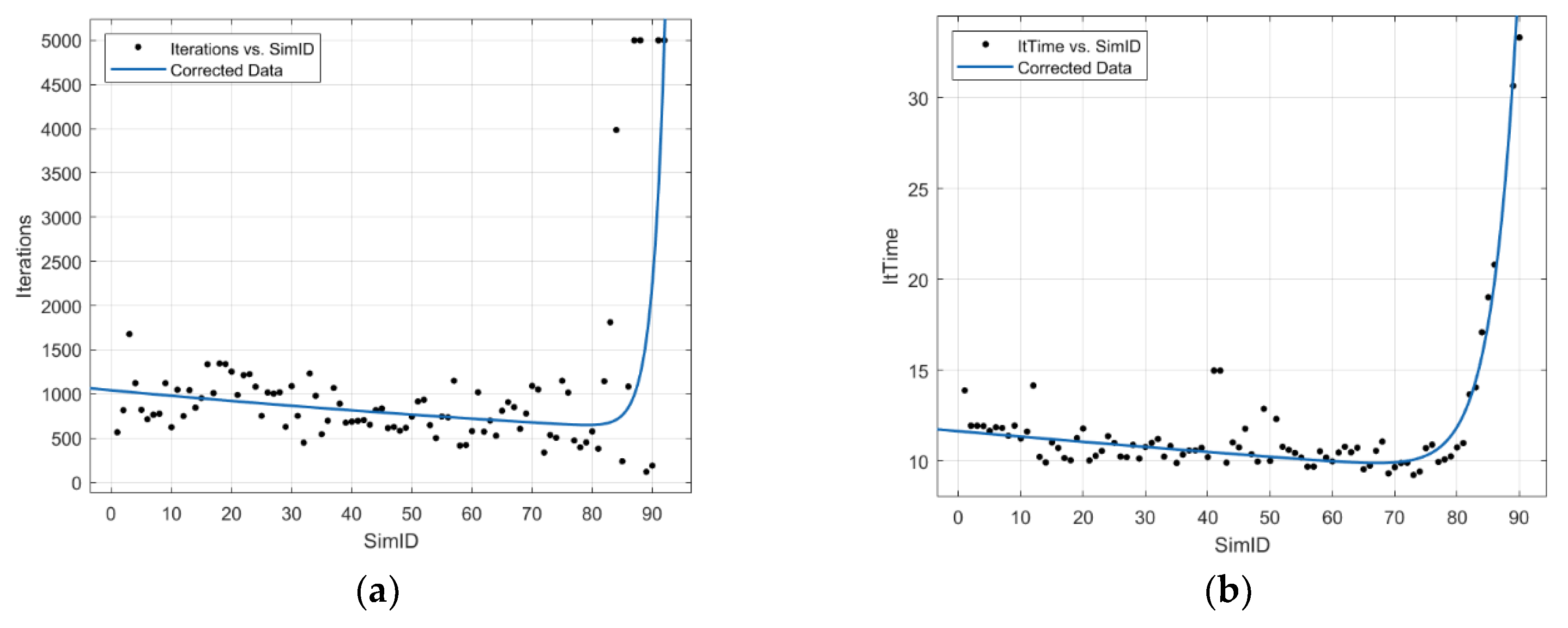
Figure 6. Comparison of the iterations and time per iteration in every TO. (a) Sim. ID vs Iterations graph: dots are the discrete data and blue is the corrected data. (b) Sim. ID vs Mean Iteration Time: dots are the discrete data and blue is the corrected data.
Preprints 109083 g006
Figure 7. Comparison of the measure of non-discreteness and machinability in every TO. (a) Non-Discreteness vs Sim. ID: dots are the discrete data and blue is the corrected data. (b) Machinability vs Sim. ID: dots are the discrete data and blue is the corrected data.
Preprints 109083 g007
Figure 8. Comparison of Machinability and Measure of Non-Discreteness. Dots are the discrete data, and blue is the corrected data.
Preprints 109083 g008
Figure 9. Comparison of Sim. ID and objective function results. Dots are the discrete data and blue is the corrected data.
Preprints 109083 g009
Figure 11. Machining filter step-by-step in x direction. (a) Initial blueprint design. (b) Highlighted in pink, the elements covered by the filter radii. (c) First column filtering. (d) Design after first column filtering. (e) Elements detection for subsequent columns (second column represented). (f) Filtering of subsequent columns (second column represented). (g) Design after second column filtering. (h) Final design after filtering.
Preprints 109083 g011
Figure 12. Geometrical parameters of the ellipsoid for obtaining its radius from the cartesian coordinates of the elements being analyzed.
Preprints 109083 g012
Table 1. Chosen study filter radius, the reason of the choice of these radii and the percentage of the elements in maximum direction that represents the radii. OS=Other Studies. ED=Euclidean Distance. LV=Large Values.
R 1.5 1.8 2 2.45 2.5 2.9 3 3.4 3.47 3.5 3.8 4
Reason OS ED ED ED ED ED OS ED ED ED ED ED
R 4.2 4.4 4.5 4.7 5 5.2 6 8 10 15 20
Reason ED ED ED ED ED ED OS LV LV LV LV
Table 2. Comparative relevant data of the verification cases.
Case (a) Case (b) Case (c) Case (d) Case (e) Case (f) Case (g)
Iterations 1018 1738 346 2086 1087 2639 790
Mnd 21.5065 0.8477 28.3512 3.901 1.1824 5.2443 6.1459
Machinability 89.577 94.381 95.751 100 95.479 100 100
Compliance 38.0111 19.5020 59.1714 136.4004 21.1516 46.4197 34.3937
Disclaimer/Publisher’s Note: The statements, opinions and data contained in all publications are solely those of the individual author(s) and contributor(s) and not of MDPI and/or the editor(s). MDPI and/or the editor(s) disclaim responsibility for any injury to people or property resulting from any ideas, methods, instructions or products referred to in the content.
Copyright: This open access article is published under a Creative Commons CC BY 4.0 license, which permit the free download, distribution, and reuse, provided that the author and preprint are cited in any reuse.
Prerpints.org logo

Preprints.org is a free preprint server supported by MDPI in Basel, Switzerland.

Subscribe

© 2024 MDPI (Basel, Switzerland) unless otherwise stated