1. Introduction
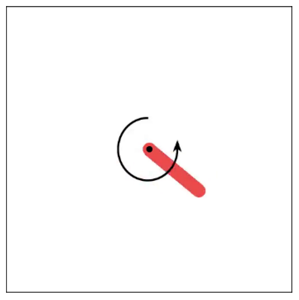
The author has been investigating a reinforcement learning approach for training neural networks using evolutionary algorithms. For instance, the author previously reported an experimental result of evolutionary reinforcement learning of neural network controllers for the pendulum task [
1,
2,
3,
4]. In these previous studies, a conventional multilayer perceptron was employed in which connection weights were real numbers. On the contrary, researchers are exploring neural networks in which the weights are discrete values rather than real numbers, accompanied by the corresponding learning methodologies [
5,
6,
7,
8,
9,
10,
11,
12].
An advantage of discrete neural networks lies in their ability to reduce the memory footprint required for storing trained models. For instance, when employing binarization as a discretization method, only 1 bit is needed for each connection weight, compared to 32 or 64 bits required for a real-valued weight. This results in a memory size reduction of 1/64 (1.56%) or 1/32 (3.13%) per connection. Given the presence of numerous connections in deep neural networks, the memory size reduction achieved through discretization becomes more pronounced, facilitating the implementation of large network models on memory-constrained edge devices. However, the performance of discrete neural networks on modelling nonlinear functions falls below that of real-valued neural networks with the same model size. To achieve comparable performance to real-valued neural networks, it is necessary for discrete neural networks to increase its model size. As the model size increases, so does the memory footprint, introducing a trade-off between memory size reduction through discretization. In other words, to maximize the effect of memory size reduction achieved through neural network discretization, it is essential to limit the increase in model size while simultaneously minimizing the number of bits per connection weight.
In this study, the author experimentally applies Genetic Algorithm [
13,
14,
15,
16] to the reinforcement training of binary neural networks and compares the result with the previous experimental result [
17] in which, instead of GA, Evolution Strategy [
18,
19,
20] was applied. In both studies, the same pendulum control task is utilized.
4. Training of Binary Neural Networks by Genetic Algorithm
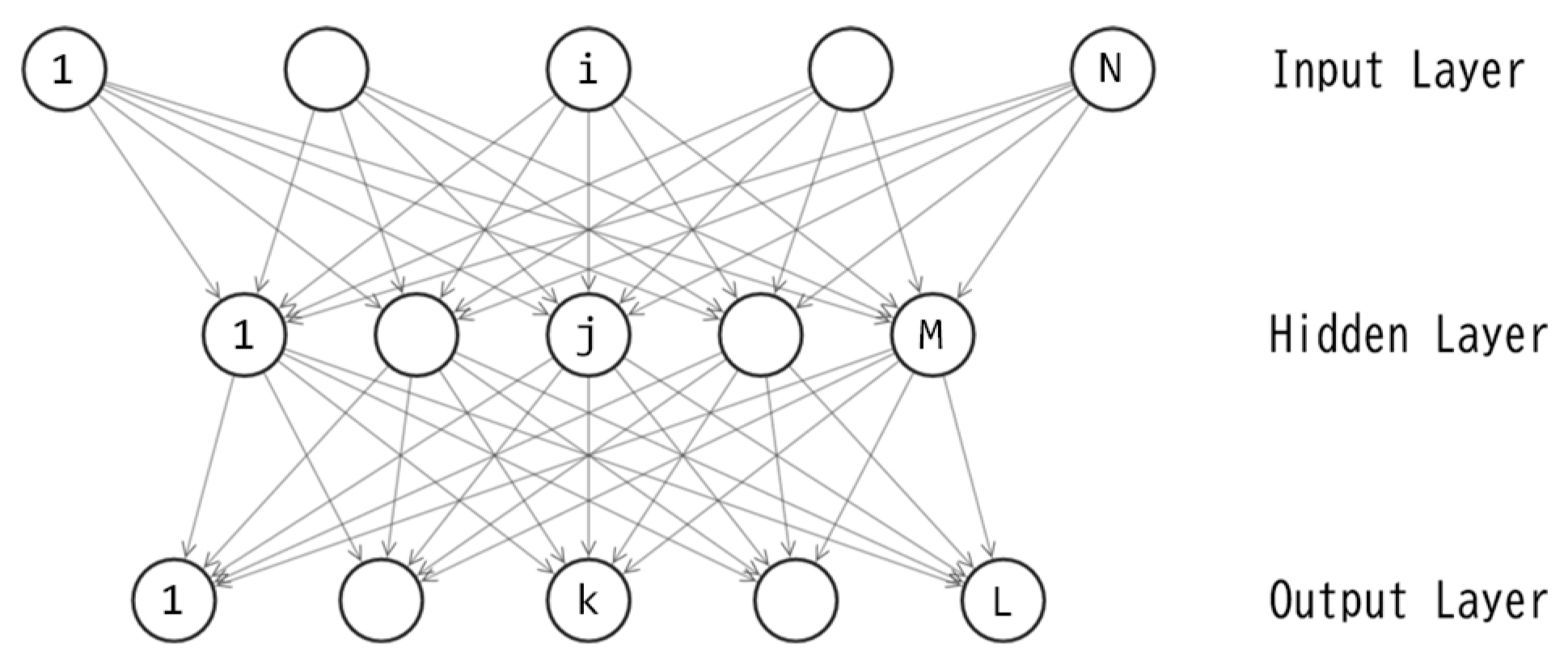
A three-layered binary perceptron, as depicted in
Figure 2, includes M+L unit biases and NM+ML connection weights, resulting in a total of M+L+NM+ML parameters. Let D represent the quantity M+L+NM+ML. For this study, the author sets N=3 and L=1, leading to D=5M+1. The training of this perceptron is essentially an optimization of the D-dimensional binary vector. Let
denote the D-dimensional vector, where each
corresponds to one of the D parameters in the perceptron. In this study, each
is a binary variable, e.g.
{-1,1} or
{0,1}. By applying the value of each element in
to its corresponding connection weight or unit bias, the feedforward calculations can be processed.
In this study, the binary vector
is optimized using Genetic Algorithm [
13,
14,
15,
16]. GA treats
as a chromosome (a genotype vector) and applies evolutionary operators to manipulate it. The fitness of
is evaluated based on eq. (1) described in the previous article [
1].
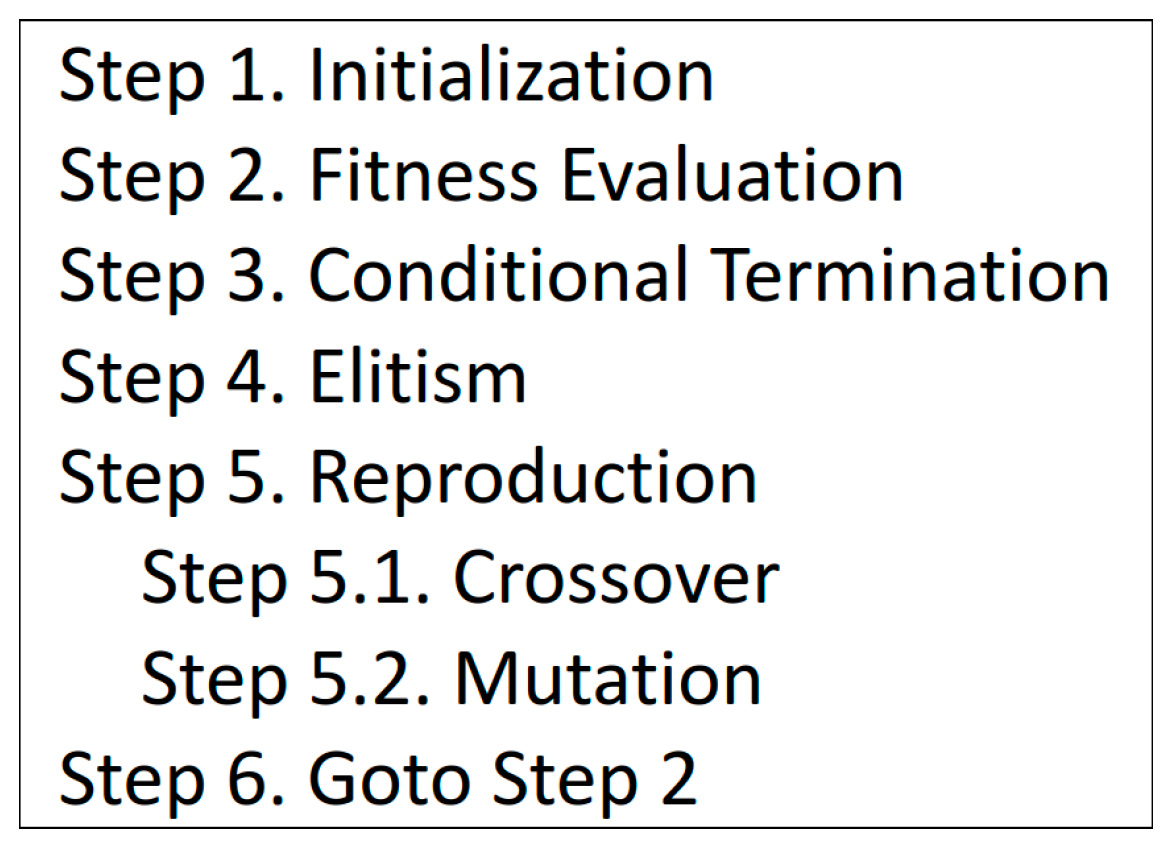
Figure 3 illustrates the GA process. In Step 1, D-dimensional binary vectors
are randomly initialized where P denotes the population size. A larger value of P promotes exploration more. In Step 2, binary values in each vector
(
) are applied to the MLP and the MLP controls the pendulum for a single episode with 200 time steps. The fitness of
is then evaluated with the result of the episode. In Step 3, the loop of evolutionary training is finished if a preset condition is met. A simple example of the condition is the maximum number of fitness evaluations.
Elites are the best E vectors among all offsprings evaluated so far, where E denotes the size of elite population. To exploit around the good solutions found so far, elite vectors are kept as parent candidates for the crossover. The elite population is empty at first. In Step 4, members in the elite population, are updated. Step 5 consists of the crossover and the mutation. In Step 5.1, new offspring vectors are produced by applying the crossover operator to the union of the elite vectors and the vectors in the current population. A single crossover with two parents produces two new offsprings, where the two parents are randomly selected from the union of and To produce new offspring vectors, the crossover is performed times. Each vector in the union of and can be selected as a parent two or more times (several vectors in the union may not be selected any time). The new offspring vectors replace the population Crossover operators applicable to binary chromosomes are a single-point crossover, a multi-point crossover and the uniform crossover. The uniform crossover is applied in this study. In Step 5.2, each element in the new offspring vectors is bit-flipped under the mutation probability pm. A greater pm promotes explorative search more.
5. Experiment
In the previous study where the binary MLPs were trained using ES, the number of fitness evaluations included in a single run was set to 5,000 [
17]. The number of new offsprings generated per generation was either of (a)10 or (b)50. The number of generations for each case of (a) or (b) was 500 and 100 respectively. The total number of fitness evaluations were 10 × 500 = 5,000 for (a) and 50 × 100 = 5,000 for (b). The experiments in this study where the binary MLPs are trained using GA employ the same configurations. The hyperparameter configurations for GA are shown in
Table 1. The mutation probability pm is set to 1/D where D denotes the length of a binary genotype vector.
Sets of two values such as {-1,1} or {0,1} can be used for the binary connection weights. The author first presents experimental results using {-1,1}. In the previous study using ES, the author tested three options, M=16, 32, and 64, for the number of hidden units. The same options are employed in this study using GA.
Table 2 presents the best, worst, average, and median fitness scores of the trained MLPs across the 11 runs. Each of the two hyperparameter configurations (a) and (b) in
Table 1 was applied. A larger value is better in
Table 2 with a maximum of 1.0.
To investigate which of the two configurations (a) or (b) is superior, the Wilcoxon signed-rank test was applied to the 12
2 data points presented in
Table 2. This test revealed that the configuration (a) is superior to the configuration (b) with a statistical significance (p<.01). Thus, reducing the population size and increasing the number of generations is more favorable than the opposite approach. This finding is consistent with that in previous study [
17] using ES; although no statistically significant difference was observed between the configurations (a) and (b), the configuration (a) was slightly superior to the configuration (b). A greater number of generations would contribute better than a greater population size in these two studies, because the length of genotype vectors (i.e., the value of D) is large and thus fine-tuning the genotype vectors repetitively in the later generations improves the MLP performance well.
Next, the author examines whether there is a statistically significant difference in the performances among the three MLPs with the different numbers of hidden units M. For each M of 16, 32, and 64, the author conducted 11 runs using the configuration (a), resulting in 11 fitness scores. The Wilcoxon rank sum test was applied to the 11
3 data points. The results showed that there was little difference between M=64 and M=32 (p=.47). While there was no significant difference between M=16 and either M=32 or M=64 (with p-values of 0.057 and 0.396, respectively), the proximity of the p-values to 0.05 indicated that M=16 performed much worse than M=32. Thus, M=32 exhibited superior performance to M=16 and little difference to M=64. Therefore, from the perspective of the trade-off between performance and memory size, the most desirable number of hidden units was found to be 32. This result is consistent with the previous study using ES [
17].
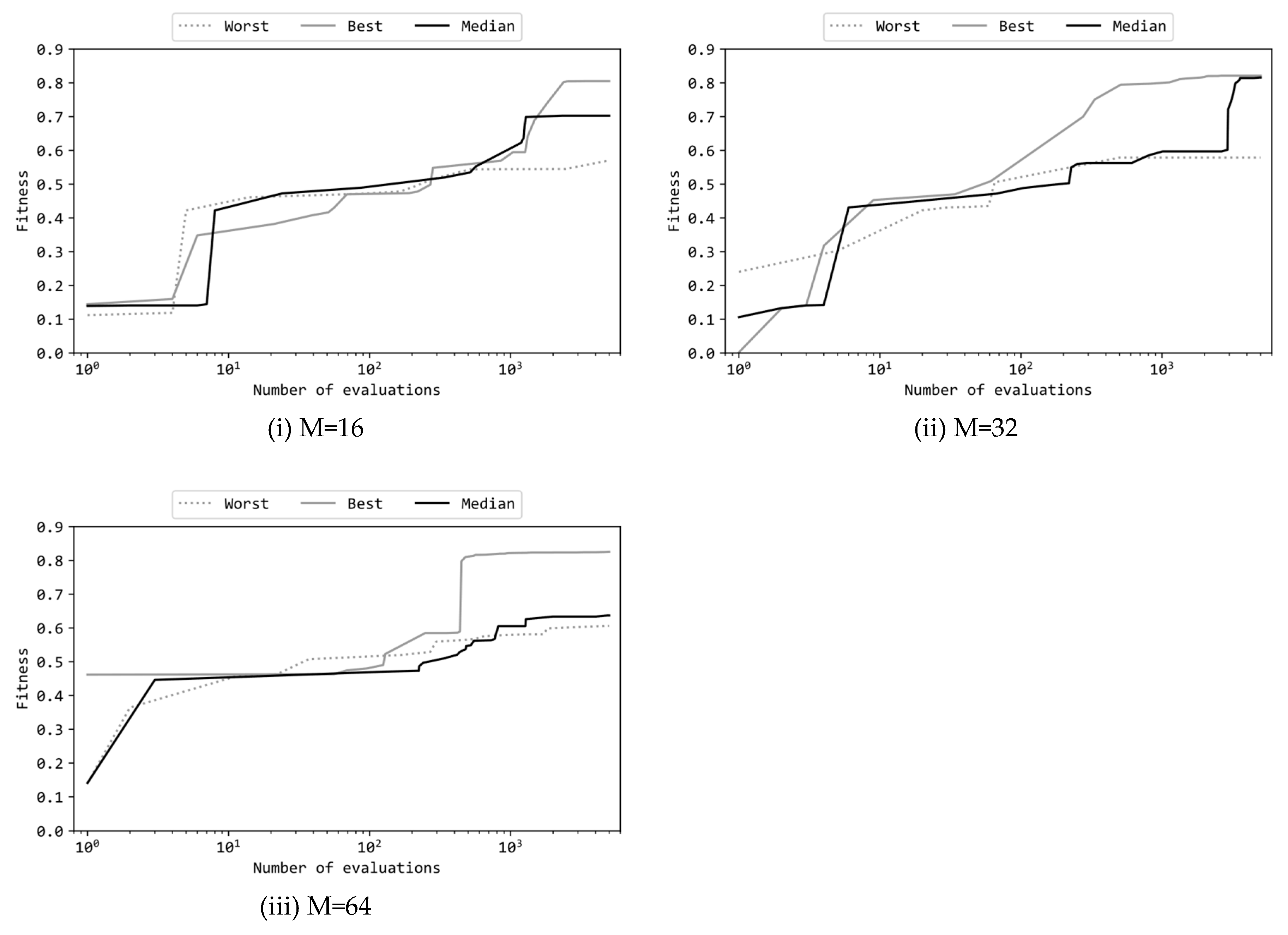
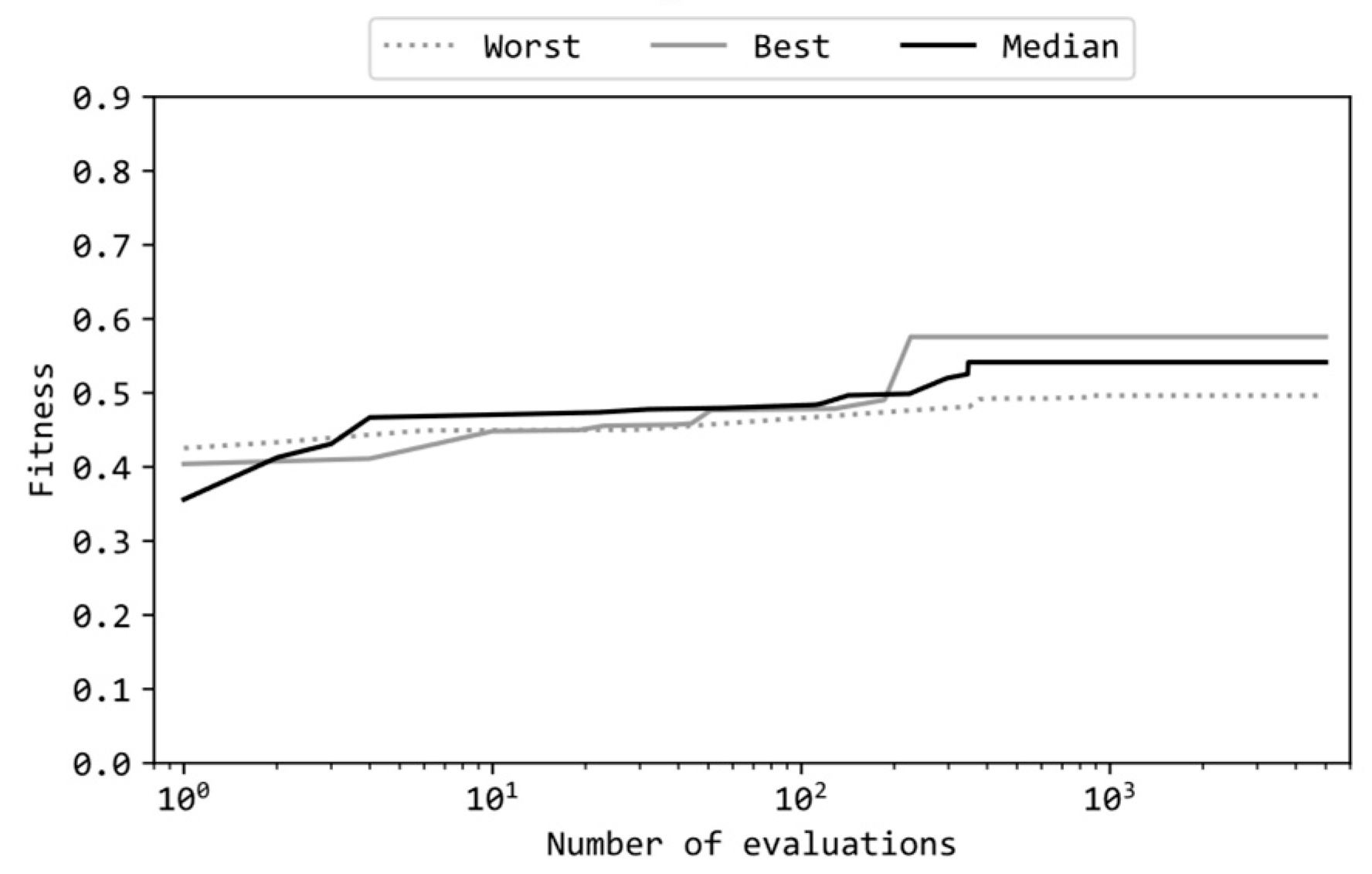
Figure 4 presents learning curves of the best, median, and worst runs among the 11 runs where the configuration (a) was applied. Note that the horizontal axis of these graphs is in a logarithmic scale.
Figure 4(i), (ii), and (iii) depict learning curves of MLPs with different numbers of hidden units (M=16, 32, 64). The curves in
Figure 4(i), (ii), and (iii) exhibit similar shapes to the corresponding figures in the previous article [
17]; each curve started around a fitness value of 0.1 and rose to approximately 0.5 within the first 10 to 100 evaluations. Subsequently, over the remaining approximately 4900 evaluations (roughly 490 generations), the fitness values increased from around 0.5 to around 0.8. However, in all cases (i), (ii), and (iii), the worst runs did not show an increase in fitness from around 0.5, indicating a failure to achieve the task. The reason for the significant difference between the best and worst runs would be due to the configuration (a) which promotes local search over global search, thus leading to some runs falling into local optima as a result of insufficient exploration of the search space. Particularly, when the number of hidden units M is set to 64, it can be observed that the performance of the median run (0.637) is as low as that of the worst run (0.606), indicating six or more failed runs. This can be attributed to the fact that as M increases, so does D, expanding the solution space extensively, thereby making failures due to insufficient global exploration more likely to occur.
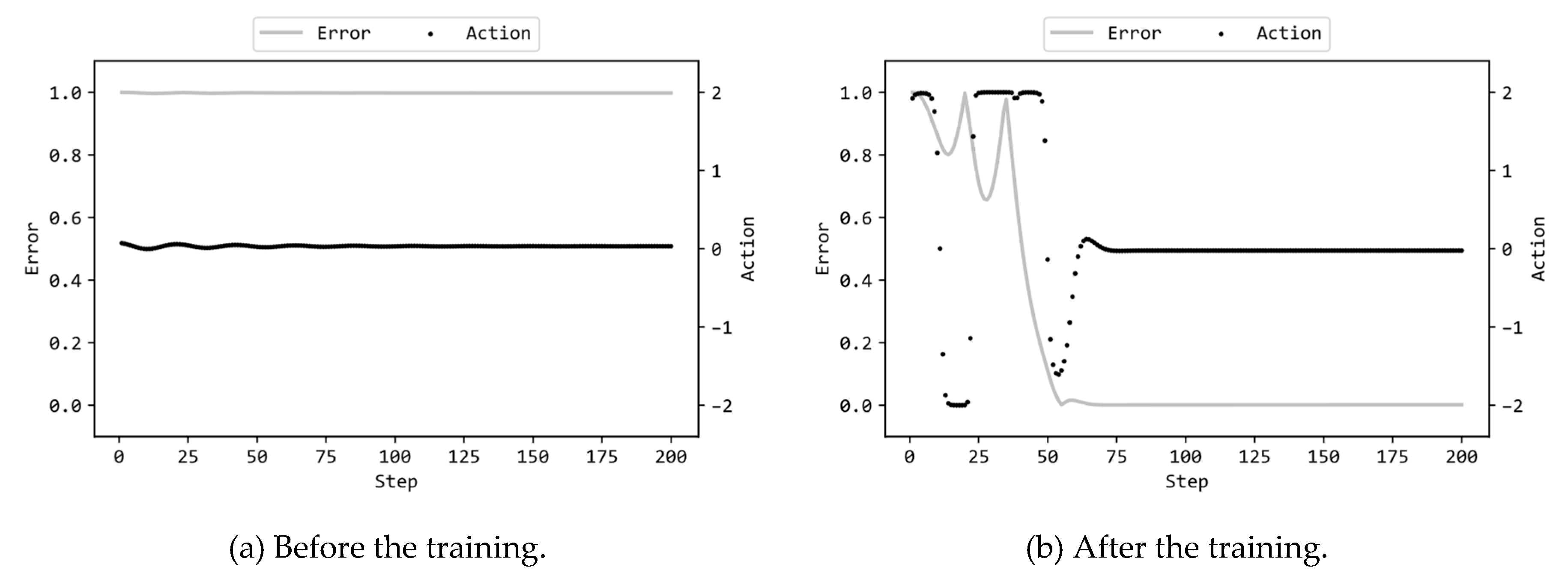
Figure 5(a) illustrates the actions by the MLP and the errors of the pendulum to the target state (values of Error(t) defined in the previous article [
1]) in the 200 steps prior to training, while
Figure 5(b) displays the corresponding actions and errors after training. In this scenario, the MLP included 32 hidden units, and GA utilized the configuration (a) in
Table 1. Supplementary videos are provided which demonstrate the motions of the pendulum controlled by the MLPs before/after trained
2,3.
Figure 5(a)(b) in this article closely resemble
Figure 6(a)(b) previously published in [
17]. For details on the figures, readers are referred to the previous article [
17] on the study using ES. These figures showed that, regardless of whether GA or ES was employed for the evolutionary training, the trained MLPs swiftly inverted the pendulum and subsequently maintained it in an inverted position with nearly zero torque.
The above reported the experimental result where {-1,1} were used as the binary values for the connection weights. The author next presents the experimental result using {0,1} instead of {-1,1}. A connection with a weight of 0 is equivalent to be disconnected, signifying its redundancy. Therefore, the presence of numerous connections with the weight of 0 implies a lighter feedforward computation for the neural network.
Table 3 presents the best, worst, average, and median fitness scores of the trained MLPs across the 11 runs. Based on the results with {-1,1}, the number of hidden units in the MLP was set to 32 and GA utilized the configuration (a) in
Table 1. Comparing
Table 3 with
Table 2 reveals that the values in
Table 3 are consistently smaller than their corresponding values in
Table 2. Thus, the performance of MLPs with {0,1} weights are inferior to those with {-1,1} weights. The Wilcoxon rank sum test to the 11 fitness scores for each case reveals that this difference is statistically significant (p < .01). This result aligns with those obtained using ES [
17], which suggests that, irrespective of the evolutionary algorithm employed for training, the performance of trained binary MLPs will be better when {-1,1} is used instead of {0,1}. Verification using other algorithms and other tasks remains future work. Furthermore, evaluating the performance when using a ternary {-1,0,1} instead of binary {-1,1} or {0,1} is also a subject for future investigation.
Figure 6 illustrates the learning curves of the MLP with {0,1} weights in the same format as
Figure 4.
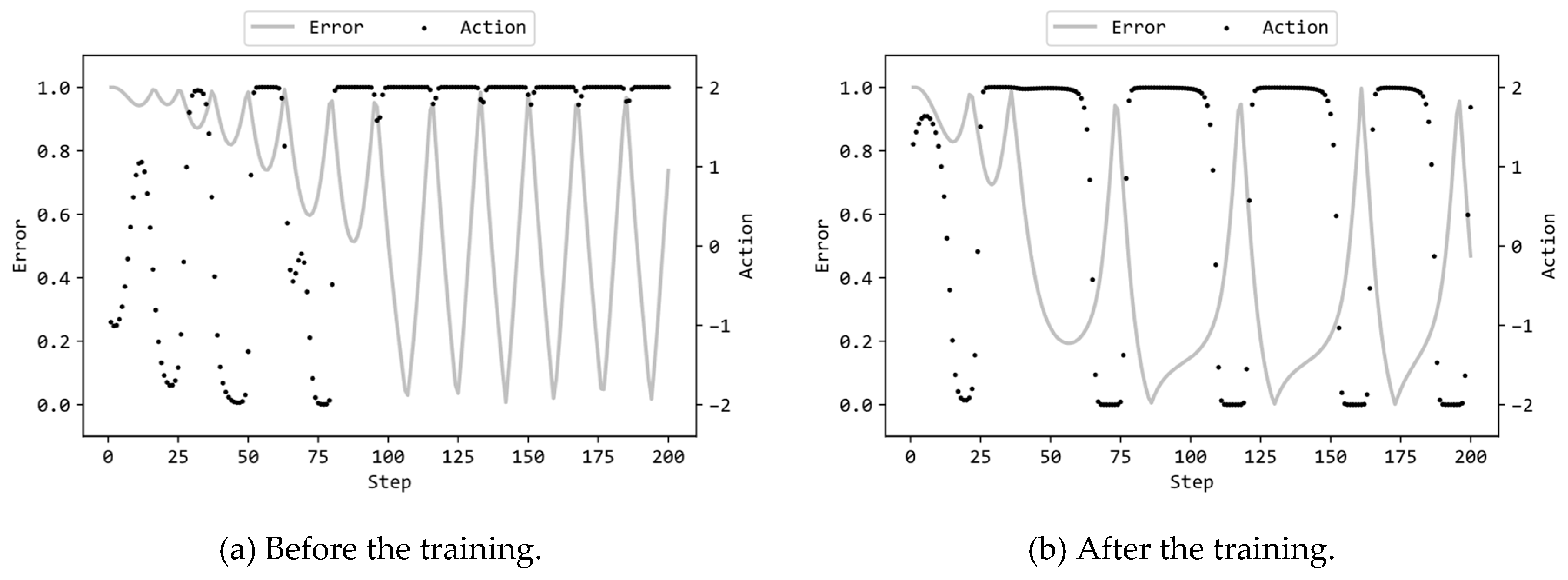
Figure 7 illustrate the actions by the {0,1} MLPs and the errors of the pendulum to the target state, in the same format as
Figure 5. The MLP included 32 hidden units, and GA utilized the configuration (a) in
Table 1. Theses figures are also quite similar to the corresponding figures by the previous study using ES [
17]. Therefore, the insights described in the previous article [
17] regarding the observations gleaned from these figures are applicable to the experimental results presented in this article. For a detailed examination of these insights, readers are encouraged to refer to the previous article [
17]. Supplementary videos are provided which demonstrate the motions of the pendulum controlled by the {0,1} MLPs before/after trained
4,5.
