Principal Component Analysis of Arctic Sea Ice Using Multi-spectral Sentinel-2 and RADAR Sentinel-1 Data

1. Introduction

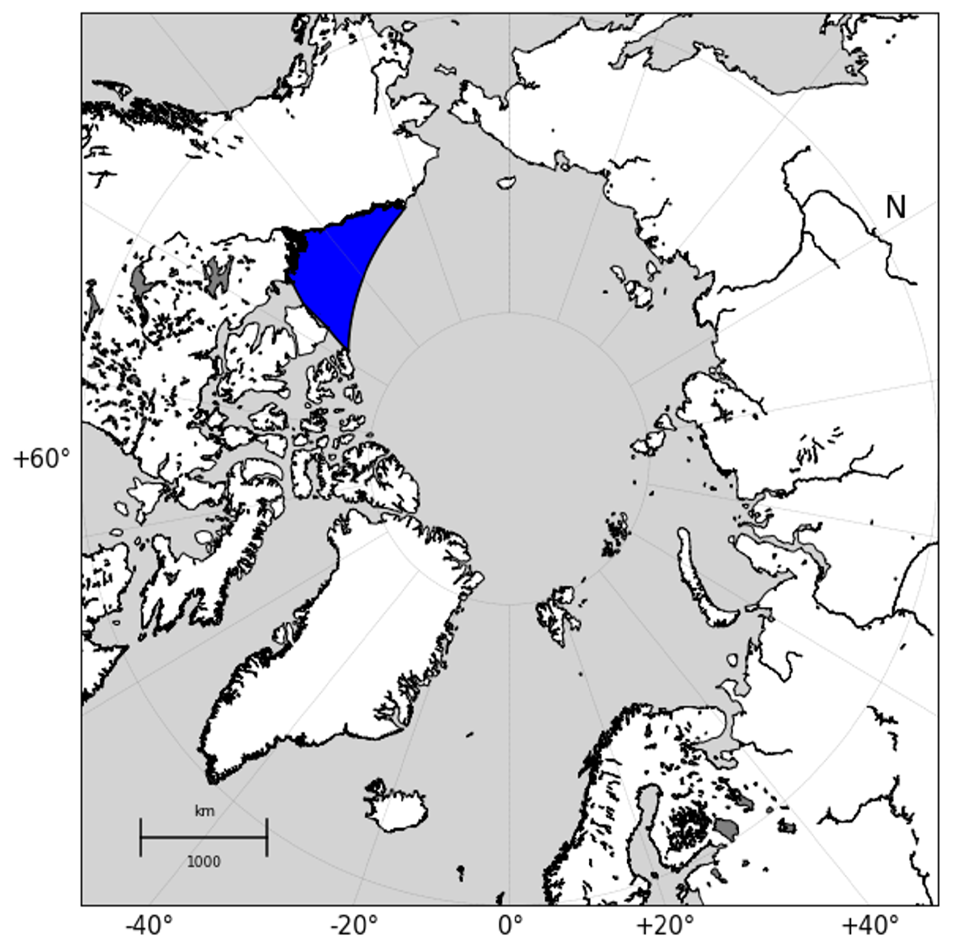
Leads are described as linear kinematic features found on sea ice surfaces. The formation of leads is akin to the process of plate tectonics, where shifting ice sheets diverge, converge and slide against each other, forming fissures in the ice. Leads are important to arctic habitats and wildlife (Stirling, 1997), polar navigation (Lasserre, 2015) and global climate (Hutter, 2018). Leads are important regulators of heat in the Arctic, with open water and thin ice leads providing the first and second largest heat fluxes into the atmosphere (approximately 600 W.m-2 and 5 W.m-2 respectively, (Maykut 1982 and Li, 2020). Radar satellite imagery is used to observe and quantify the changes in lead fractions across the ice sheet. Radar data is particularly useful in quantifying lead fractions since the instrument can make observations in Polar regions regardless of weather conditions or time of year (Lindsay and Rothrock, 1995), (Röhrs and Kaleschke, 2012), (Bröhan and Kalesche, 2014), (Willmes and Heinemann, 2015). Still, Sentinel-1’s dual polarization technique is limited in its bands for the performance of a PCA, we instead look at the changes in the ice surface during polar daytime when optical images can be captured. Multi-spectral imagers are useful instruments, especially for validation techniques. Optical satellites, such as Sentinel-1’s sister constellation: Sentinel-2, provides true color image representations of our ice scenes. These images represent the reflection of light on the Earth’s surface, whose bands encapsulate energy at specific wavelength intervals (Van der Meer, et al., 2014). Sentinel-2 data boasts a 12 band composite spanning across the visible and infrared wavelengths. The dynamic spatial and spectral nature of the optical imagery provides a suitable basis on which a principal component analysis may be conducted (Wakulińska and Marcinkowska-Ochtyra, 2020).Therefore, we exercise this technique to extract information over an ice scene (dated: April 20, 2020) and classify the image, based on the composite’s strongest signals in its first to third components. Google Earth Engine (GEE) hosts a large repository of satellite data, including the entire Sentinel catalog. GEE has been used in several research arenas, from vegetation and land use mapping (Gorelick et al., 2017 and Tsai, et al., 2018) to wetland and snow melt detection (Gulácsi, et al., 2020 and Liang et., al, 2021). Indeed, GEE and Sentinel-2 are proven powerhouses in the use of remote sensing techniques and climate observations in cloud computation environments. Currently, there are no studies published focusing on the detection of leads in the Arctic using this platform which provide a solution to the common big data problem of data storage and computation power. This study provides a principal component technique to sea ice classification in the GEE cloud computation environment using Sentinel-2 optical data. The Beaufort Gyre (Figure 1), once described as an ice production area has shown a decrease in productivity with increased climate forcing over the last decade (Armitage, 2020). This motivates our investigation of sea ice lead prevalence during the lifetime of the Sentinel 1 and 2 instruments. The aim of this study is to classify sea ice open water and thin ice leads in the offshore Alaskan region in the Beaufort Gyre to assess the changes over the ice sheet.

2. Methods

2.1. Sentinel-1 Classification Scheme

The lead detection algorithm uses co-and cross-polarized image channels (HH-HV) from the Sentinel-1 satellite and is described in Williams et al., (2024). Artificial data is created by using the product of the HH and HV bands, which is then used as a tri-false color image composite. Training data is created by labelling thick ice and open water leads since they are the most visually discernible in both optical and SAR images. This is because thick ice is bright white and leads are dark, elongated fissures in the ice surface. Thin ice fractions and ridges are more ambiguous since they are shades of grey and bright white elongated features. Ridges are a specific concern, since in windy conditions, leads can also appear bright. Texture features are extracted from the mean signal co-polar (HH) band, since it contains the highest power signal and is less interfered with by noise than with the cross-polar band (HV). A 7x7 gaussian window is used to analyze the image in blocks and a simple non-iterative clustering technique (SNIC) is used, which is a built-in function in Google Earth Engine. The SNIC is used for image segmentation, to cluster similar spectral regions and subsequently outline geometries in the ice field. The texture features are discerned using the contrast, variance, entropy and angular second moment, where:

Variance = ${{\sum }_{i,j=1}^{N}P}_{i,j}$$\left(i-{\mu }_i\right)$² & ${{\sum }_{i,j=1}^{N}P}_{i,j}$$\left(i-{\mu }_j\right)$²

Contrast = ${{\sum }_{i,j=1}^{N}P}_{i,j}$ $(i-j)$²

Entropy = ${{\sum }_{i,j=1}^{N}P}_{i,j}$ $\left(-ln\left(P_{i,j}\right)\right)$

ASM = ${\sum }_{i,j=1}^N{P}_{i,j}^2$

Where P is the probability of the matrix, (i,j), in which the pixel value µ  is the mean pixel value of the matrix (Fausi, et al., 2020). The ice classes are visually inspected and labelled with visual aid from the Sentinel-2 images. This, along with the resultant texture features provide our training sample for our support vector machine learning technique. Open water and thin ice leads are separated using their elongated features, compared with other features that do not result from deformational forces. The training and test image ratio is 40-60% for which, the image composites are classified using the support vector machine classifier.

2.2. Sentinel-2 Classification Scheme

The Sentinel-2 classification scheme requires less image correction techniques as described in Williams et al., (2024) since the multi-spectral imagery provides true color images of the ice scene. Sentinel-2 is comprised of 2 satellites, Sentinel-2A and 2B, with a third satellite (2C) to be launched in 2024. The multispectral imager provides 12 bands in the visible, near-infrared, and short-wave infrared spectrum. Sentinel-2 operates at 10-,20- and 60-meter resolutions. However, the central wavelengths of each band for Sentinel-2 and Landsat-8 are different. In fact, S2A and S2B differ in wavelength and bandwidth, although by a negligible margin (up to  3 nm). False RGB images are used instead of true color images to enhance the water bodies in the sea ice scenes. Therefore, instead of red-blue-green images, we use red-near-infrared-blue images. This increases the contrast between water features (open water lead covered areas) and non-water body features (e.g. thick ice, ridges. We also use the Q60 cloud masking convention in Google Earth Engine to minimize the effects of atmospheric interference in the classification technique. All images with greater than 90% cloud cover is automatically removed from the selection within our region of interest (the Beaufort Sea). Image labelling, texture analysis, segmentation, training and testing sampling are done the same as in the Sentinel-1 classification scheme. The support vector machine learning technique as described is also applied, using 7 bands available in Sentinel-2 to classify open water leads in the scene.

2.3. Google Colab Python Environment

Alongside the use of GEE for data retrieval, preparation and classification, we opt to use Google Colab, a cloud computation python environment. Google Colab (GC) is an exceptional tool for the use of superior python functions in the cloud, minimizing the pressure of data storage while simultaneously enhancing processing power through parallelization. GC allows the user to mount their Google Drive storage point to the environment, allowing easy data imports and exports of results.

2.4. Python Modules

• from datetime import datetime
• import pandas as pd
• import geopandas as gpd
• import numpy as np
• import matplotlib.pyplot as plt
• from matplotlib import cm
• import matplotlib.cbook
• from mpl_toolkits.basemap import Basemap
• import random
• from mpl_toolkits.axes_grid1 import make_axes_locatable
• from scipy import stats
• import matplotlib.image as mpimg
• from sklearn.metrics import r_2score
• from sklearn.decomposition import PCA
• import warnings

2.5. Principal Component Analysis

The PCA method is such that the first component will always contain the most variation found in the original data. This is referred to as the “integrated brightness” and provides a good index of the general image characteristics. In the case of sea ice data, the image scenes may be water or ice dominant. The second component then highlights the major differences between the image channels. In fact, it is suggested that studies using multitemporal monthly data over an annual cycle display a second component that tracks the seasonal evolution well (Piwowar, et al., 1996). Principal components three and onward usually represent increasingly local variation and anomalies. Therefore, we propose that it is within these variations that the open water and thin ice leads may be characterized since the creation of new ice is variable depending primarily on atmospheric conditions.

2.6. Plotting Techniques

The results of the principal component analysis yield mean and anomalous digital signals from the false RGB color composite images. From this, we can visualize these parameters graphically in image plots as well as quantitatively in scatter plots to display the orthogonal components. The mean and standard deviations will give a margin of error of the spectral boundaries of the lead types versus the ice ridges in the image scenes which can be both spectrally and geometrically similar.

3. Results

The onset freezing period in the Arctic begins in Fall season (October), with peak freeze occurring in the December-February months. Therefore, this period captures the optimum sea ice available in SAR scenes. Mosaics of daily sea ice scenes are used to derive the total sea ice area for the December – February 2020 period. Generally, the area covered is marked by an abundance of thick sea ice cover. However, as thin ice is generated within the gyre producing more material for congelation, (example julian day: 351), the thick ice area is diminished until it is consolidated (example julian: 353). This is characteristic of the evolution of sea ice, particularly during the freeze-up period (December). 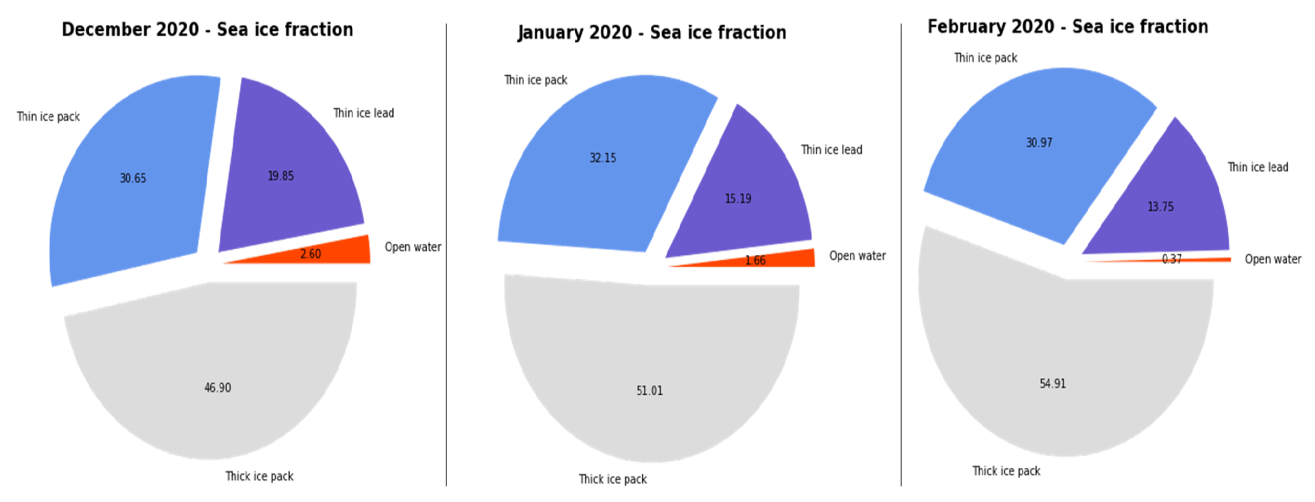Figure 2 displays the monthly sea ice fraction for the 2020 winter period. The Figure shows that, more than fifty percent (50%) of the sea ice cover is characterized by thick ice, followed by thin ice features. In contrast, the open water segment is negligible; not exceeding three percent (3%).

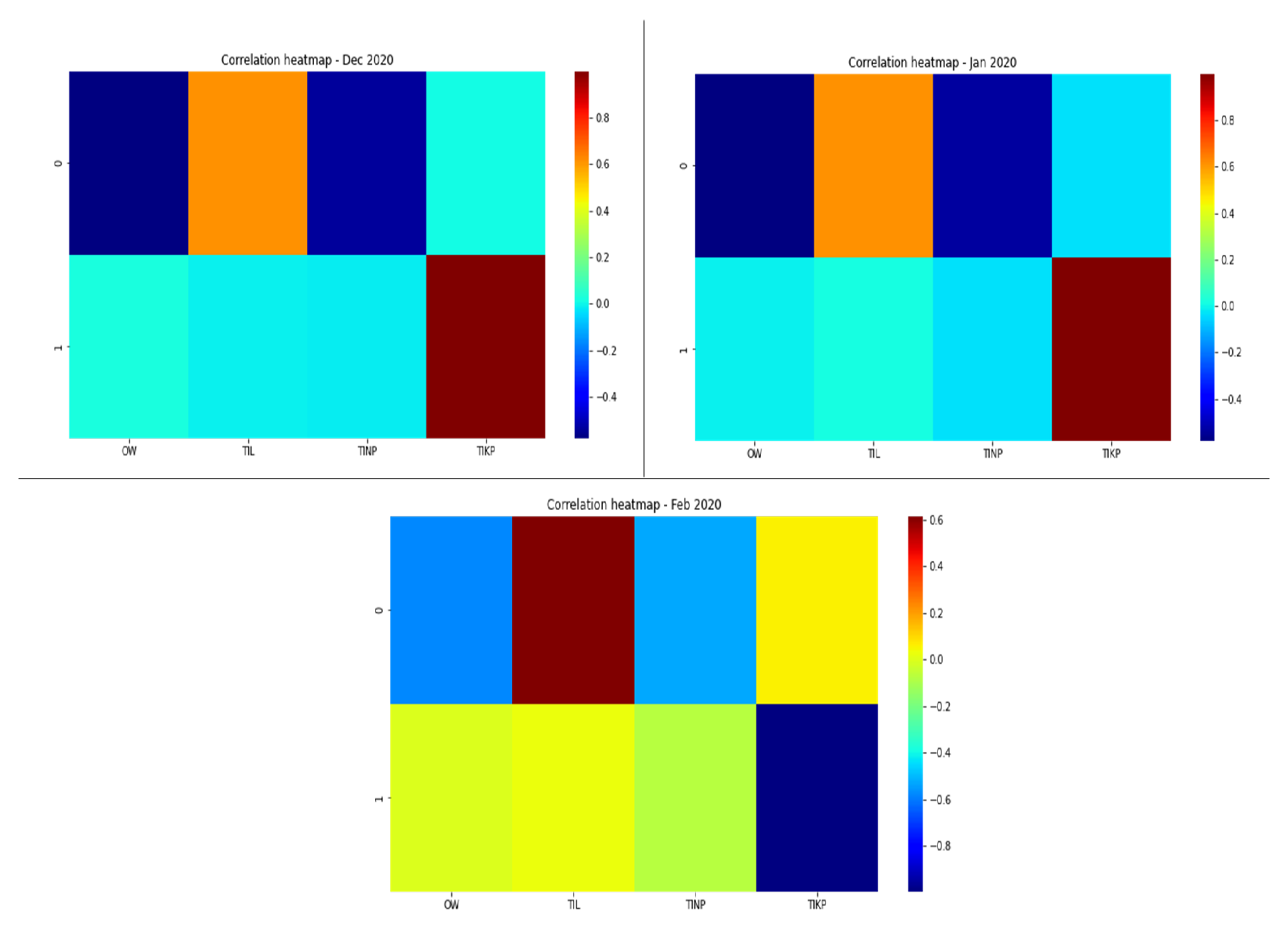
The principal component analysis reveals more information about these scenes. Figure 3 illustrates the correlation matrix of the first and second components (0 and 1 respectively) with respect to the classified sea ice types. December and January show an inversely related relationship in the first component with respect to open water and the thin ice pack while a direct relationship exists in the second component regarding the thin ice leads and thick ice pack. However, by February the strong inverse relationship shown in the open water and thin ice pack is diminished, while the thin ice lead positive correlation in the first component becomes stronger. In staunch contrast, the thick ice pack in the second component is inverted to a very strong negative relationship. Intuitively, the onset of the freezing period is dominated by open water and thin ice components while thick ice is less prominent at this time. The first component not only confirms the genesis of juvenile ice types, but further proports the strong prevalence of thin ice leads. Maximum freezing in February shows a shift in the dominance of the thin ice pack and open water segments, with an increase in thin ice leads. This relationship is definitive of the evolution of sea ice during peak freezing and by extension, the heat budgetary constraints in the Beaufort Sea region. In February, there is a higher production of thin ice leads with decreasing thin packed ice, suggesting that lead areas are actively opening during this time without further production of new ice. This is marked by the limited open water available to produce young ice for congelation. The ice surface during this time is dominated by a mosaic of thick ice and thin ice leads with less coverage of open water and thin packed ice.

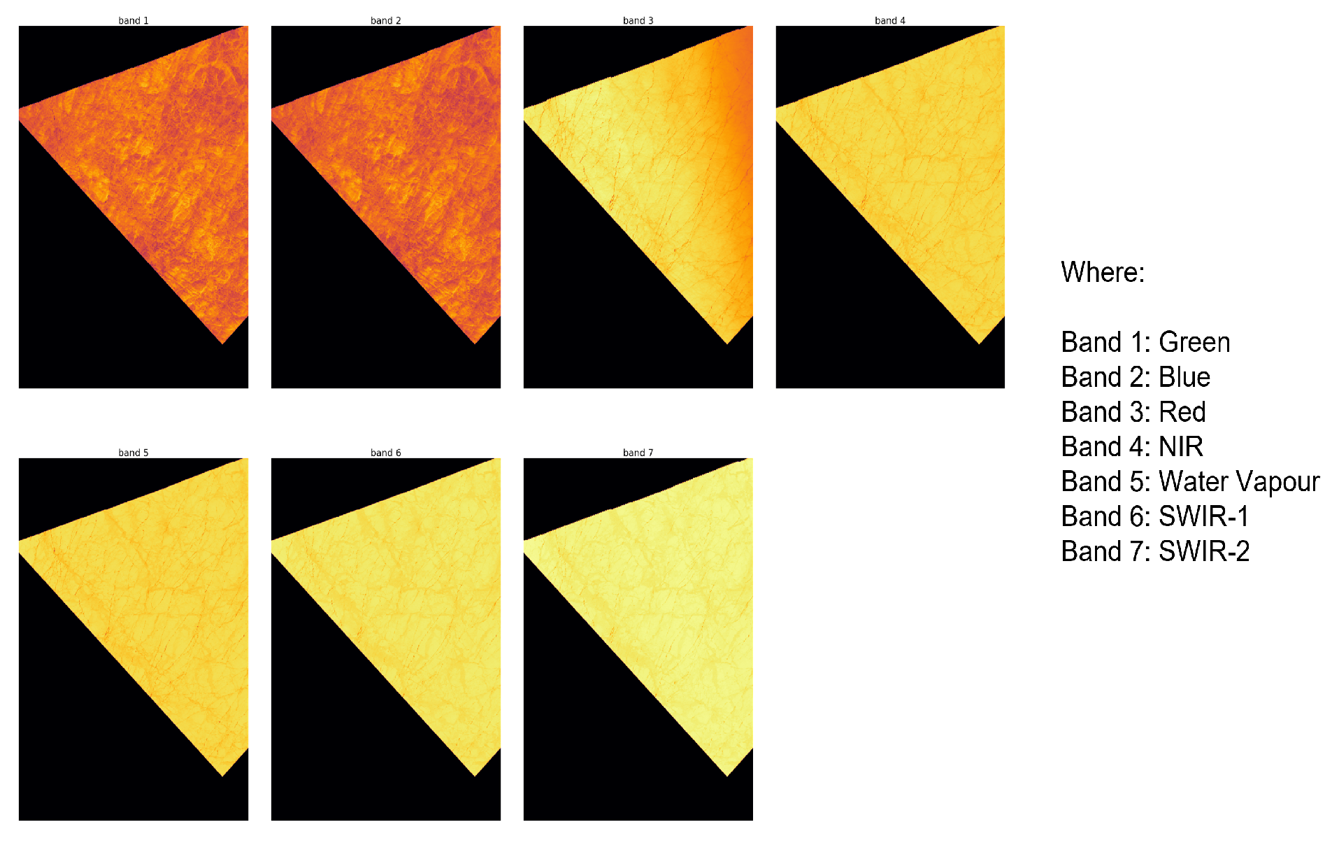
Figure 4 shows an image sample of a Sentinel-2 image with elongate features across the ice scene. The green, blue, red, near-infrared (NIR), water vapour and shortwave-infrared (SWIR) 1 and 2 bands are selected since they are most useful in dectecting water logged areas.

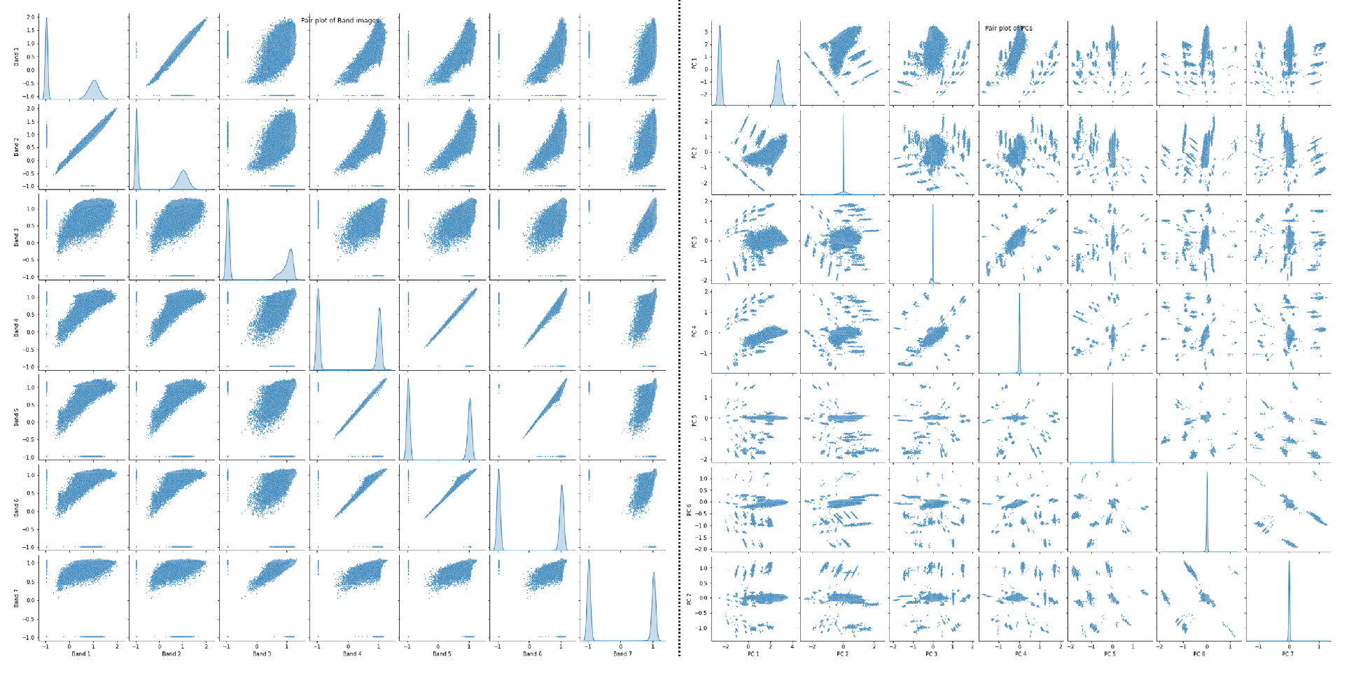
Pair plots of the corresponding bands and the prinicipal components are shown in Figure 5. The plots reveal the variance and correlations between the datasets. While the first component contains the most prominent information from the data, the other components describe other useful information. Bands with similar information (shortwave-infrared and near-infrared) show less variance between themselves. Of course, more variance exists where bands with greater difference in wavelengths (e.g. green and red bands).

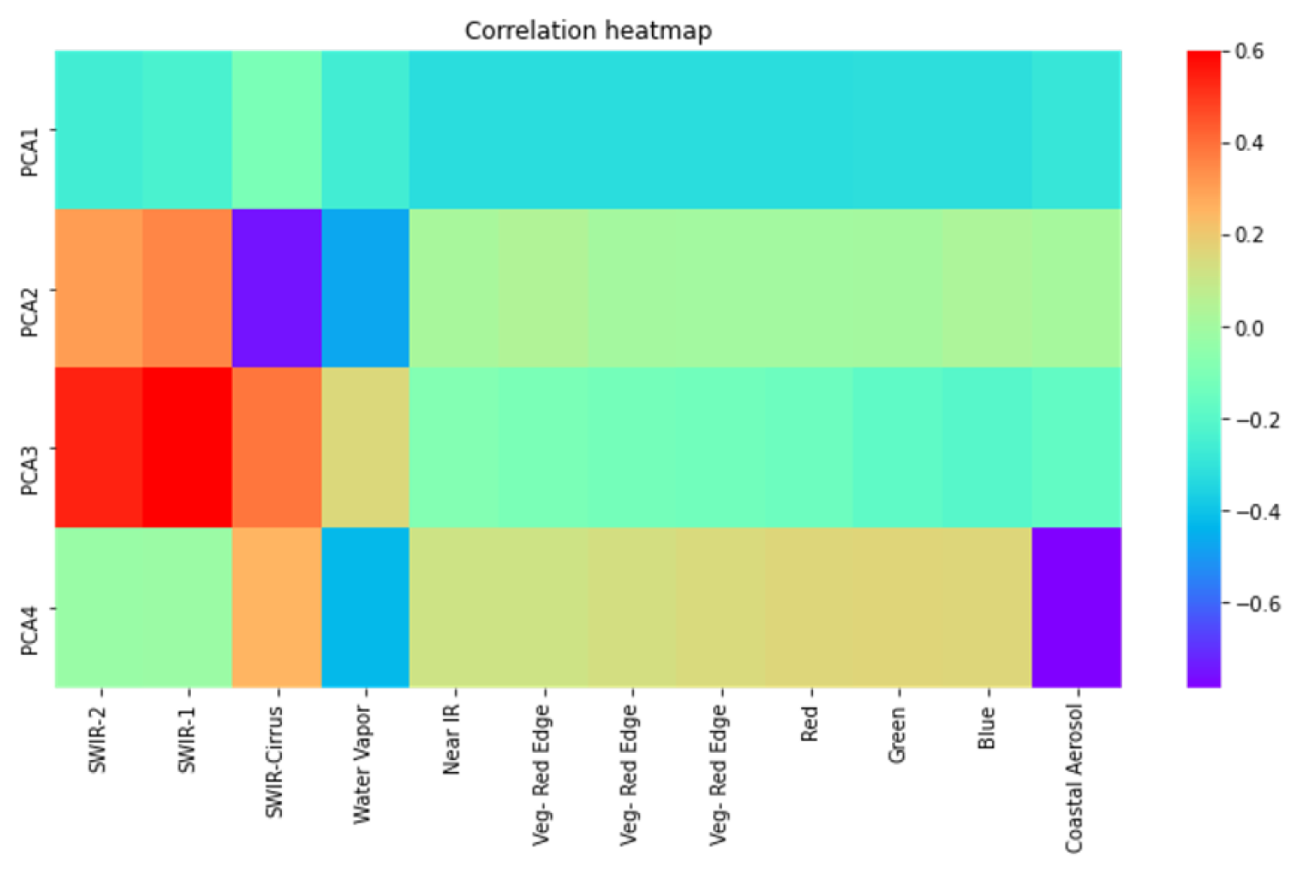
A correlation heat map is shown in Figure 6. The map describes an ice dominant scene that is covered with open water lead features. The heat map shows low correlations in the first component, which represents the most dominant feature in the image. This is expected since the images analyzed are during the frost maximum period of that year. However, the second and third components show higher correlations, with the highest correlations being described by the third component. The highest correlations with the third component are the shortwave-infrared bands. The forth component also describes higher correlations with the red and shortwave-infrared bands. This suggests that the third and forth components contain information regarding open water features, since the red and infrared bands are used in remote sensing to denote areas that are waterlogged. Figure 7 shows the reconstructed image using the four principal components described. The image composite shows a highly textured surface, comprised of thick ice, with elongate features that represent open water leads (thin blue lines) as well as ridges (thin white lines). Other features in the image can be described as undifferentiated ice types.

4. Conclusions

Winter scenes in the Arctic describe the cyclical nature of sea ice from their inception at the onset freezing to the peak freezing period. The principal component analysis defines the dominant ice type in the region as thin packed ice and leads for most of the winter period. The thick ice is the next dominant feature in the scenes, shifting from a strongly positive to negative relationship in the second component from freezing onset to its maximum. In terms of heat regulation in the Arctic, this suggests that the total heat budget is dominated by a latent heat flux rather than a sensible heat flux where heat exchange is incident on the sea ice surface. The evolution of the dominant ice types is critical to understanding the potential energy changes in the Arctic. As open water and thin ice lead extent changes so does the regulatory heat energy. Therefore, a time series analysis of the sea ice types is necessary to estimate the Arctic heat budget.

References

- Armitage, T., Manucharyan, G., Petty, A., Kwok, R., and Thompson, A. (2020). Enhanced eddy activity in the Beaufort Gyre in response to sea ice loss. Nature Communications, 11(1). [CrossRef]
- Bröhan, D., Kaleschke, L., & Notz, D. (2014). Analysis of Arctic sea-ice leads from Advanced Microwave Scanning Radiometer.
- Gorelick, N., Hancher, M., Dixon, M., Ilyushchenko, S., Thau, D., and Moore, R. (2017). Google Earth Engine: Planetary-scale geospatial analysis for everyone. Remote Sensing Of Environment, 202, 18-27. [CrossRef]
- Gulácsi, A., and Kovács, F. (2020). Sentinel-1-Imagery-Based High-Resolution Water Cover Detection on Wetlands, Aided by Google Earth Engine. Remote Sensing, 12(10), 1614. [CrossRef]
- Hutter, N., Zampieri, L., and Losch, M. (2018). Leads and ridges in Arctic sea ice from RGPS data and a new tracking algorithm. The Cryosphere Discussions, 1-27. [CrossRef]
- Lasserre, F. (2014). Simulations of shipping along Arctic routes: comparison, analysis and economic perspectives. Polar Record, 51, 239 - 259.
- Li, X., Krueger, S. K., Strong, C., Mace, G. G., and Benson, S. (2020). Midwinter Arctic leads form and dissipate low clouds. Nature Communications, 11(1), 1-8.
- Liang, D., Guo, H., Zhang, L., Cheng, Y., Zhu, Q., and Liu, X. (2021). Time-series snowmelt detection over the Antarctic using Sentinel-1 SAR images on Google Earth Engine. Remote Sensing Of Environment, 256, 112318. [CrossRef]
- Lindsay, R., and Rothrock, D. (1995). Arctic sea ice leads from advanced very high resolution radiometer images. Journal of Geophysical Research, 100(C3), 4533. [CrossRef]
- Maykut, G.A. (1982). Large-scale heat exchange and ice production in the central Arctic. Journal of Geophysical Research, 87, 7971-7984.
- Piwowar, J., and LeDrew, E. (1996). Principal Components Analysis of Arctic Ice Conditions between 1978 and 1987 as Observed from the SMMR Data Record. Canadian Journal Of Remote Sensing, 22(4), 390-403. [CrossRef]
- Röhrs, J., and Kaleschke, L. (2012). An algorithm to detect sea ice leads by using AMSR-E passive microwave imagery. The Cryosphere, 6(2), 343-352. [CrossRef]
- Stirling, I. (1997). The importance of polynyas, ice edges, and leads to marine mammals and birds. Journal Of Marine Systems, 10(1-4), 9-21. [CrossRef]
- Tsai, Y., Stow, D., Chen, H., Lewison, R., An, L., and Shi, L. (2018). Mapping Vegetation and Land Use Types in Fanjingshan National Nature Reserve Using Google Earth Engine. Remote Sensing, 10(6), 927. [CrossRef]
- Wakulinska, M., & Marcinkowska-Ochtyra, A. (2020). Multi-Temporal Sentinel-2 Data in Classification of Mountain Vegetation. Remote. Sens., 12, 2696.
- Williams, J. C.; Ackley, S. F.; Mestas-Nuñez, A. M.; Macdonald, G. J. Lead Detection with Sentinel-1 in the Beaufort Gyre using Google Earth Engine. Preprints 2024, 2024050284. [CrossRef]
- Willmes, S. and Heinemann, G. (2015). Sea-Ice Wintertime Lead Frequencies and Regional Characteristics in the Arctic, 2003–2015. Remote Sensing, 8(1), 4. [CrossRef]