An Online Identification Method for Mechanical Parameters of Dual-Inertia Servo System

Preprint

Article

An Online Identification Method for Mechanical Parameters of Dual-Inertia Servo System

Altmetrics

Downloads

Views

Comments

Kai Liu^*,

Kai Liu^*,

This version is not peer-reviewed

Submitted:

14 June 2024

Posted:

17 June 2024

You are already at the latest version

Alerts

Abstract

In a dual-inertia system based on permanent magnet synchronous motor (PMSM), the elastic transmission mechanism, such as reducer and coupling, is prone to mechanical resonance, which reduces the precision of servo system transmission. Model prediction and introduction of state feedback are effective methods to suppress mechanical resonance, but the control parameters de-pend on the mechanical parameters of the system. Therefore, mechanical parameter identification is very necessary. In this paper, a forgetting factor recursive least square method is used to identify the mechanical parameters of the dual-inertia elastic system. Firstly, the mathematical model of the dual-inertia system is established and reasonably simplified. Then, the discrete function of the identification algorithm is constructed, and the motor speed and electromagnetic torque are sam-pled to achieve the on-line identification of the main mechanical parameters of the dual-inertia system, and the influencing factors of the identification accuracy are analyzed. Finally, simulations and experiments are carried out to verify the effectiveness of the algorithm.

Keywords:

Subject: Engineering - Electrical and Electronic Engineering

1. Introduction

In the design of servo drive system controllers, in order to achieve a better response process or higher positioning accuracy, the controller parameter tuning usually needs to be substituted for mechanical parameter values. For example, in the design of a speed loop controller, the accurate rotational inertia is necessary. Otherwise, mismatched parameters will lead to slow dynamic response or poor steady-state performance of the system [1]. Manufacturer’s production differences or variations in operating conditions may cause changes in the mechanical parameters of the system, resulting in a decline in control performance, so it is crucial to identify the mechanical parameters of the study.

In 1956, L.A. Zadeh first put forward the concept of "identification", and then gave its definition in 1962: system identification is to determine a mathematical model equivalent to the identification system from a set of model classes based on input and output observations of the identification system [2]. Since then, domestic and foreign parameter identification technology has developed rapidly, and related algorithms have been applied to the field of motor drive by scholars.

Parameters in a servo drive system include internal electrical parameters (resistance, inductance, magnetic chain, etc.) and external mechanical parameters (rotational inertia, friction damping, drive shaft stiffness, etc.), where the internal parameters are used for the design of a current loop controller, and the external parameters are used for the design of a speed loop controller. The main difference between a single-inertia and a multi-inertia system parameter identification is the difference in external mechanical parameters, and the multi-inertia system adds the mechanical parameters of the transmission mechanism in addition to the parameters of the drive motor and load. The identification algorithms of each parameter in a single-inertia system have been more mature, including acceleration and deceleration methods, least squares and improvement algorithms [3], model reference adaptive method [4], observer-based method [5], extended Kalman filtering method [6], etc. Currently, this function is available in servo drives such as Mitsubishi MR-JE-40A and Panasonic A6 [7] in Japan. The multi-inertia system parameter identification is represented by double inertia, due to the mechanical structure of the introduction of more parameters, complex working conditions and other issues appear more difficult. However, since the technology has not yet matured, the application of the method is not as rich as the single inertia system. At present, there are mainly two types of methods: parametric and non-parametric methods.

The parametric method recognizes the system parameters by assuming a system model such that the difference between its output and the actual output of the system satisfies a set performance index function. With the development of digitalization, the assumed system model has been transformed from a continuous data discrimination model to a discrete data discrimination model. Seppo E. Sarika’s team at Aalto University, Finland, used a discrete-time polynomial model with an Output Error (OE) structure in 2012 and a random binary sequence as the excitation signal. The comparisons of the identification accuracy under different test methods, such as open loop, indirect closed loop, and direct closed loop, pointed out that the identification results deviated greatly in the case of a closed loop at speed due to the influence of the controller [8]. In order to overcome the difficulties of closed-loop identification, the team proposed an improved indirect method in 2013, which used a pseudo random binary sequence (PRBS) as the excitation signal for six external mechanical parameters (drive motor inertia and friction coefficient, load motor inertia and friction coefficient, driveshaft stiffness and friction coefficient), and a random binary sequence (PRBS) as the excitation signal. PRBS (Pseudo Random Binary Sequence) as the excitation signal, combined with the least squares method, to find out the parameters in the discrete domain, and then transformed to the frequency domain through the zero-pole matching method, to obtain the identification results. However, due to its cumbersome arithmetic process, it needs to be combined with dSPACE, which limits its application in industry [9]. Literature [10] considered the different identification settings and gave simulation and experimental results for two different mechanism signals, PRBS and Chirp, under ARX and OE identification models, respectively.

The non-parametric method achieves identification based on the system response curve, such as impulse response and frequency response characteristics. Literature [11] superimposed PRBS on the stator current component i_q for system excitation without encoder, used an extended speed adaptive observer to obtain the motor rotational speed, performed signal processing, calculated the frequency response, plotted the Baud plot and obtained the resonance frequency by Welch's method. Literature [12] proposed a send generation identification method using linearized weighted overall least squares, which derived the transfer function under the premise that the system resonance characteristics were unknown and there was a time delay, and completed the fixed order based on the coefficient map to obtain the transfer function reflecting the mechanical resonance characteristics and time lag, with a high identification accuracy. However, the nonparametric identification method cannot be used for systems with serious nonlinear features, because the nonlinear features will greatly change the system frequency response, resulting in poor identification accuracy [13].

Inspired by the references, this paper firstly establishes the mathematical model of a dual-inertia servo system, secondly constructs the discrete identification function by the recursive least squares method with a forgetting factor, then realizes the on-line identification of the main mechanical parameters and at the same time analyses the influencing factors of the identification accuracy, and finally proves the validity of the identification algorithm by simulation and experiment.

2. Mathematical Modelling of Dual Inertia Systems

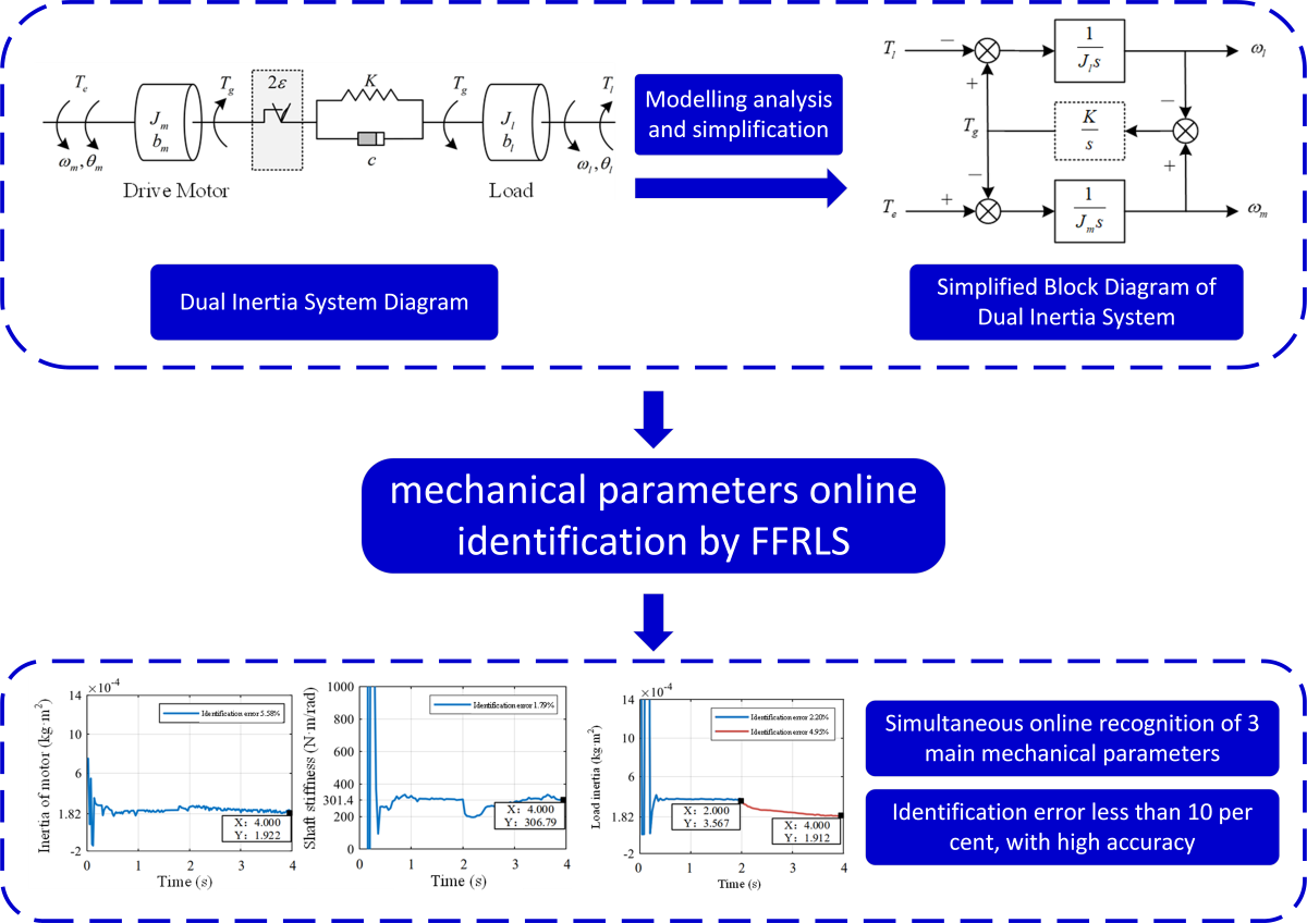
In a dual-inertia system, the drive motor and the load are connected via a driveshaft with a torsional stiffness of K, a damping coefficient of c, a clearance of 2ε, and a simplified ratio of 1, as shown in Figure 1.

Considering that the effect of the gap is mainly reflected in the initial position of non-engagement or changes in the direction of motion to produce positioning errors, while in the identification of mechanical parameters can be maintained in one direction of rotation, necessarily engaged. Therefore, the clearance only has an effect at the initial stage of identification and does not affect the final iteration results. Neglecting the gap, the coupling inertia, the damping coefficient of each part, that is, the mechanical parameters to be identified are simplified as the drive motor inertia J_m, the coupling stiffness K and load inertia J_l, and analyze the motion process of each inertial body in the double inertia system to establish a mathematical model: when the drive is given a current to generate the electromagnetic torque T_e, which drives the drive motor with rotational inertia of J_m to rotate, and the load side is static due to the inertia, and the existence of the angular difference that This causes the drive shaft to twist and deform, generating a transfer torque. This torque is both the load torque of the drive motor and the driving torque of the load, which acts together with the load-side torque T_l to determine the load speed. The mathematical model of the above process is as follows:

\{\begin{array}{l} J_{m} {\ddot{θ}}_{m} = T_{e} - T_{g} \\ J_{l} {\ddot{θ}}_{l} = T_{g} - T_{l} \\ ω_{m} = {\dot{θ}}_{m} \\ ω_{l} = {\dot{θ}}_{l} \\ T_{g} = K (θ_{m} - θ_{l}) \end{array}

(1)

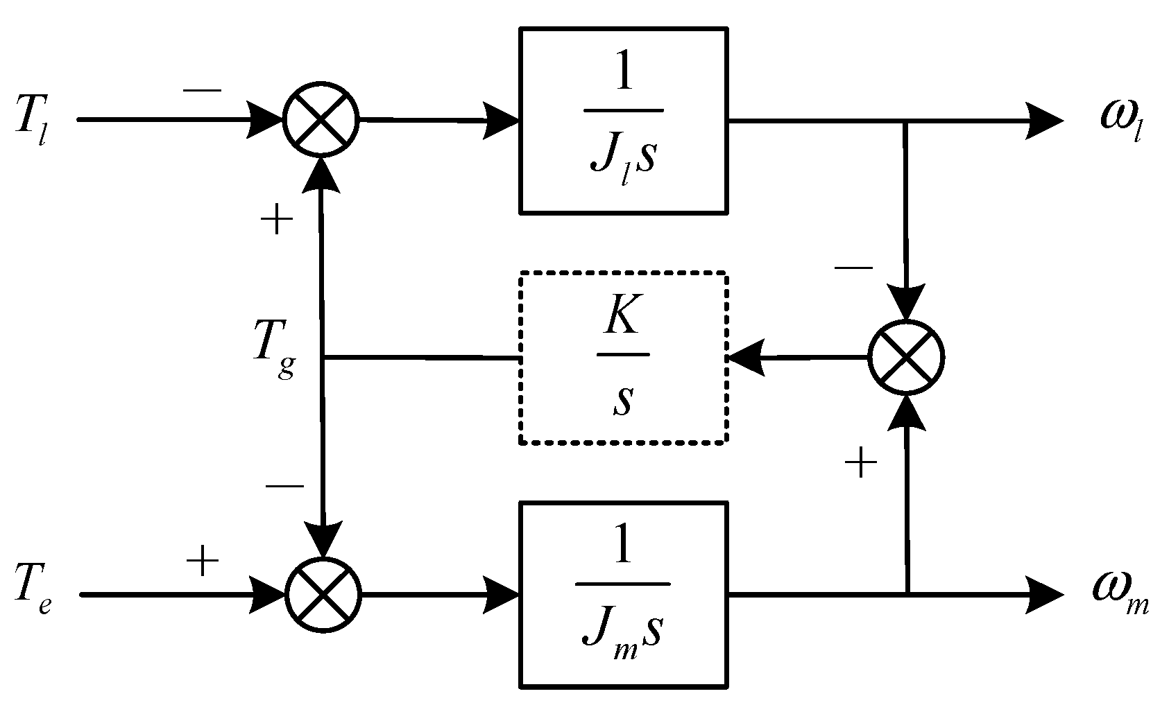
A simplified block diagram of the dual-inertia system is shown in Figure 2.

The motor speed is determined by the electromagnetic torque and load torque together, and its transfer function is

ω_{m} (s) = \frac{(J_{l} s^{2} + K)}{J_{m} J_{l} s^{3} + (J_{m} K + J_{l} K) s} T_{e} (s) - \frac{K}{J_{m} J_{l} s^{3} + (J_{m} K + J_{l} K) s} T_{l} (s)

(2)

where the transfer function from motor speed to electromagnetic torque is

ω_{m} (s) = \frac{(J_{l} s^{2} + K)}{J_{m} J_{l} s^{3} + (J_{m} K + J_{l} K) s} T_{e} (s)

(3)

From (3), the system exists a pair of conjugates zero poles, the conjugate zero point is the Anti-resonance Frequency (ARF), the conjugate poles are the Natural Torsional Frequency (NTF), the zero poles make the system produce a relatively strong response to the input of a specific frequency, i.e., trigger mechanical resonance. The zero pole causes the system to respond more strongly to a specific frequency input, i.e., triggering a mechanical resonance.

ω_{A R F} = \sqrt{\frac{K}{J_{l}}}

(4)

ω_{N T F} = \sqrt{\frac{J_{m} K + J_{l} K}{J_{m} J_{l}}}

(5)

3. Identification of Mechanical Parameters for Dual Inertia Systems

3.1. The Principle of Least Squares

The Least Square (LS) method was first introduced by K.F. Gauss in his work on the prediction of celestial orbits, and is based on the principle of minimizing the sum of the squares of the errors in each set of data. The n sets of input and output observations of an observable system are expressed as (6), and the estimates of the system parameters can be obtained according to the least squares method as (7).

{y (k), u (k), k = 1, 2, \dots, n}

(6)

θ = {(ϕ^{Τ} ϕ)}^{- 1} ϕ^{Τ} Y

(7)

where ϕ is the data vector matrix and Y is the system output matrix.

However, when using LS, every time an observation is added, it is necessary to re-solve the identification of the new observation together with all the previous data, which leads to a large number of repeated calculations, and the amount of data increases dramatically over time, which seriously affects the computational speed of the system. In order to improve the computational efficiency, the Recursive Least Square (RLS) algorithm is introduced, which is based on the idea of assuming that the deviation of the estimated values of the system parameters at k moments and k-1 moments is ∆, i.e.

θ (k) = θ (k - 1) + Δ

(8)

Also, by the least square’s method, the estimate for moment k is obtained as

θ (k) = {[ϕ^{T} (k) ϕ (k)]}^{- 1} ϕ^{T} (k) Y (k)

(9)

In which,

ϕ (k) = (\begin{matrix} ϕ (k - 1) \\ φ^{T} (k) \end{matrix}), Y (k) = (\begin{matrix} Y (k - 1) \\ y (k) \end{matrix})

Let the covariance matrix P(k) be

P (k) = {[P^{- 1} (k - 1) + φ (k) φ^{T} (k)]}^{- 1}

(10)

Thus,

P^{- 1} (k) = P^{- 1} (k - 1) + φ (k) φ^{T} (k)

(11)

From (9) and (10), the estimate for the k-1 moment is

θ (k - 1) = P (k - 1) ϕ^{T} (k - 1) Y (k - 1)

(12)

From (11) and (12),

ϕ^{T} (k - 1) Y (k - 1) = [P^{- 1} (k) - φ (k) φ^{T} (k)] θ (k - 1)

(13)

Thus, the estimates of the system parameters at moment k can be corrected by moment k-1 to obtain

θ (k) = P (k) ϕ^{Τ} (k) Y (k) = θ (k - 1) + K (k) [y (k) - φ^{T} (k) θ (k - 1)]

(14)

where K(k) the gain vector and K(k)=P(k)φ(k).

The iterative formula for the recursive least square’s method can be obtained from the matrix inverse lemma as well as (13) as

\{\begin{matrix} θ (k) = θ (k - 1) + K (k) [y (k) - φ^{T} (k) θ (k - 1)] \\ P (k) = [E - K (k) φ^{T} (k)] P (k - 1) \\ K (k) = P (k - 1) φ (k) / [1 + φ^{T} (k) P (k - 1) φ (k)] \end{matrix}

(15)

where E is the unit matrix. Although the RLS algorithm solves the problem of a large number of repeated calculations well, its default is that the old and new data are equally important, which will not reflect the real-time status of the motor. Therefore, the attenuation coefficient is added to RLS to weaken the influence of the old data on the discriminated values, forming the recursive least squares method with forgetting factor, and the iteration formula is modified as

\{\begin{matrix} θ (k) = θ (k - 1) + K (k) [y (k) - φ^{T} (k) θ (k - 1)] \\ P (k) = \frac{1}{λ} [E - K (k) φ^{T} (k)] P (k - 1) \\ K (k) = P (k - 1) φ (k) / [λ + φ^{T} (k) P (k - 1) φ (k)] \end{matrix}

(16)

In the formula, the value range of forgetting factor λ is usually 0.9~1. The smaller λ is, the faster the convergence speed is; the larger λ is, the smaller the fluctuation of algorithm recognition results is. After many simulations and experimental verification, λ=0.99 is finally selected for this topic.

3.2. Mechanical Parameter Identification Algorithm for Dual-Inertia Systems

In order to apply FFRLS, the system transfer function needs to be converted from the frequency domain to the discrete domain. The commonly used discretization methods [14] and their advantages and disadvantages are listed below:

(1): First-order backward difference: the mapping relationship is severely distorted, the transformation accuracy is low, and there are fewer engineering applications;
(2): First-order forward difference: the mapping relationship is severely distorted, and the stability of the system after discretization cannot be guaranteed (unless the sampling period is small);
(3): Bilinear transformation (Tustin) method: better accuracy, easy to apply, the disadvantage is that the high-frequency characteristics of the distortion is serious;
(4): Zero-pole matching method: the need to decompose the transfer function into zero-pole form, and the need for steady state gain matching, the application is not convenient enough;
(5): z-conversion method (impulse response invariant method): z-conversion is more cumbersome and prone to frequency aliasing;
(6): z-transform method with keeper: also has the disadvantages of z-transform.

Considering the frequency range of the dual-inertia system and the ease of application of the discrete method, Tustin's method is used in this topic. T_s is the discrete sampling period, the transfer function of the system in the discrete domain is obtained as

ω_{m} (z) = \frac{θ_{1} z^{3} + θ_{2} z^{2} + θ_{2} z + θ_{1}}{z^{3} + θ_{3} z^{2} - θ_{3} z - 1} T_{e} (z) - \frac{θ_{4} z^{3} + 3 θ_{4} z^{2} + 3 θ_{4} z + θ_{4}}{z^{3} + θ_{3} z^{2} - θ_{3} z - 1} T_{l} (z)

(17)

Among the above equation,

\{\begin{matrix} θ_{1} = \frac{4 J_{l} T_{s} + K T_{s}^{3}}{8 J_{m} J_{l} + 2 (J_{m} K + J_{l} K) T_{s}^{2}} \\ θ_{2} = \frac{- 4 J_{l} T_{s} + 3 K T_{s}^{3}}{8 J_{m} J_{l} + 2 (J_{m} K + J_{l} K) T_{s}^{2}} \\ θ_{3} = \frac{- 24 J_{m} J_{l} + 2 (J_{m} K + J_{l} K) T_{s}^{2}}{8 J_{m} J_{l} + 2 (J_{m} K + J_{l} K) T_{s}^{2}} \\ θ_{4} = \frac{K T_{s}^{3}}{8 J_{m} J_{l} + 2 (J_{m} K + J_{l} K) T_{s}^{2}} \end{matrix}

(18)

Convert the above equation into the expression required by FFRLS, the output ω_m(k) at k stage is

\begin{array}{l} ω_{m} (k) = θ_{1} [T_{e} (k) + T_{e} (k - 3)] + θ_{2} [T_{e} (k - 1) + T_{e} (k - 2)] \\ + θ_{3} [ω_{m} (k - 2) - ω_{m} (k - 1)] + ω_{m} (k - 3) \\ - θ_{4} [T_{l} (k) + 3 T_{l} (k - 1) + 3 T_{l} (k - 2) + T_{l} (k - 3)] \end{array}

(19)

Let the output be a parameter vector and a data vector as follows:

\begin{array}{l} θ = [θ_{1} θ_{2} θ_{3} 1 θ_{4}] T \\ ϕ = [T_{e} (k) + T_{e} (k - 3), T_{e} (k - 1) + T_{e} (k - 2), \\ - ω_{m} (k - 1) + ω_{m} (k - 2), ω_{m} (k - 3), \\ - (T_{l} (k) + 3 T_{l} (k - 1) + 3 T_{l} (k - 2) + T_{l} (k - 3))]^{T} \end{array}

(20)

The data vector consists of the sampled values of electromagnetic torque T_e, load torque T_l and motor speed ω_m, and the initial values are all set to 0. The parameter vector corresponds to five system parameters, of which the coefficient of ω_m(k-3) is always 1 and does not need to be identified, here all the initial values of the parameters are still set to 0.01 according to empirical formulas, and the final results of which can be used to judge whether the identification algorithm can converge to the true value or not; the initial value of the covariance matrix P (0) = 10⁶E(6). According to the initial value and the input and output, the results of parameter identification in the discrete domain are calculated iteratively by (16).

After the discrete domain parameter identification is completed, the equation is solved by substituting into (18) to complete the conversion of the parameters to be sought from the discrete domain to the frequency domain. The equations are solved as (21), which are all polynomials, avoiding the nonlinear operations such as ln function brought by other discrete methods, saving computational resources and parameter conversion time. It is worth noting that there are four equations and three to-be-sought mechanical parameters in (18), among which θ₄ does not need to participate in the conversion process, which means that the load torque T_l only participates in the iteration as a compensating effect without affecting the conversion process.

\{\begin{matrix} J_{m} = - \frac{T (θ_{3} - 1)}{6 θ_{1} - 2 θ_{2}} \\ J_{l} = \frac{2 T (2 θ_{1} - θ_{2} + θ_{1} θ_{3})}{(3 θ_{1} - θ_{2}) (θ_{1} + θ_{2})} \\ K = \frac{16 θ_{1} - 8 θ_{2} + 8 θ_{1} θ_{3}}{T {(3 θ_{1} - θ_{2})}^{2}} \end{matrix}

(21)

4. Simulation Verification

4.1. Algorithmic Validity

In order to verify the effectiveness of the above algorithm, the model is built and simulated in MATLAB/Simulink, and the model parameters are consistent with the experimental platform is shown in Table 1.

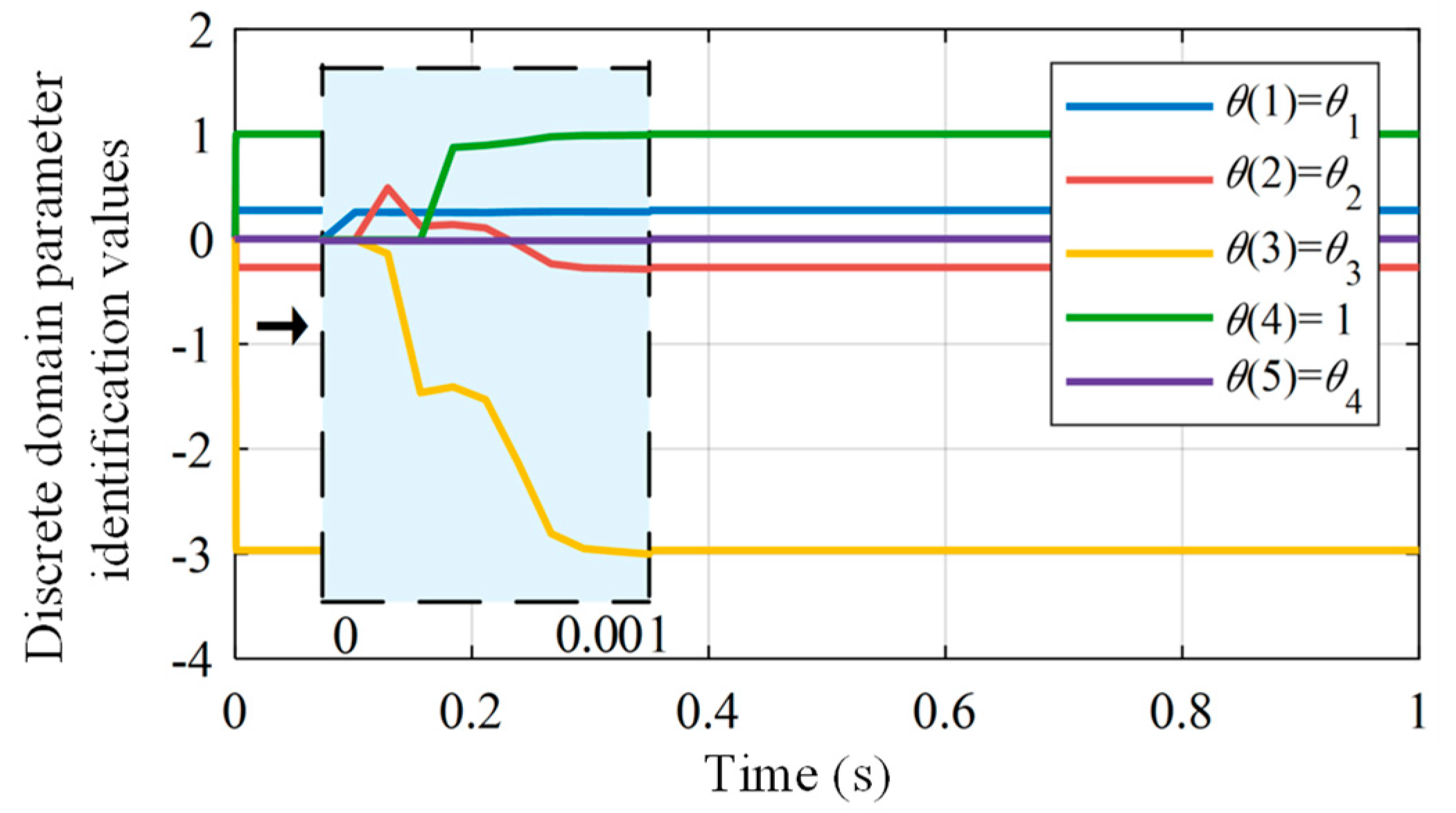
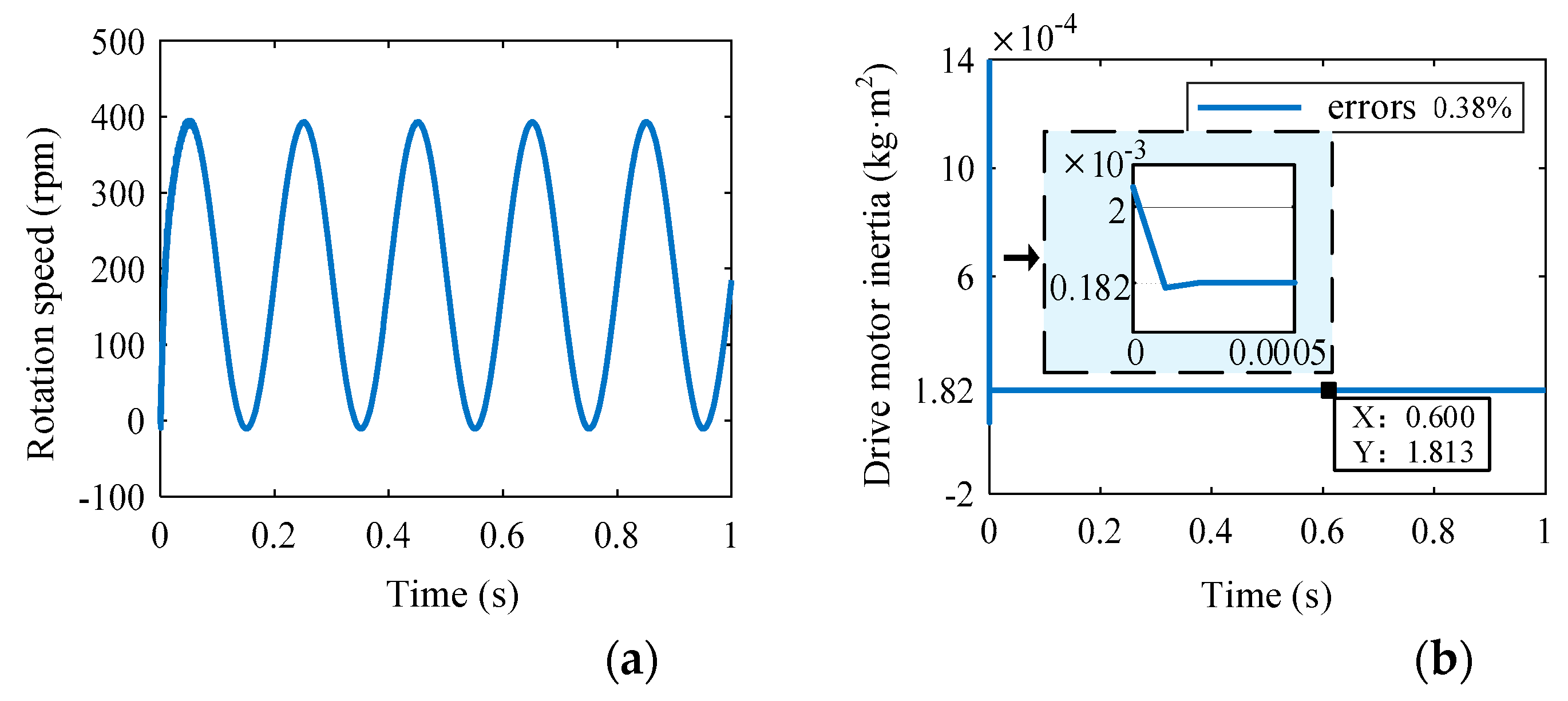
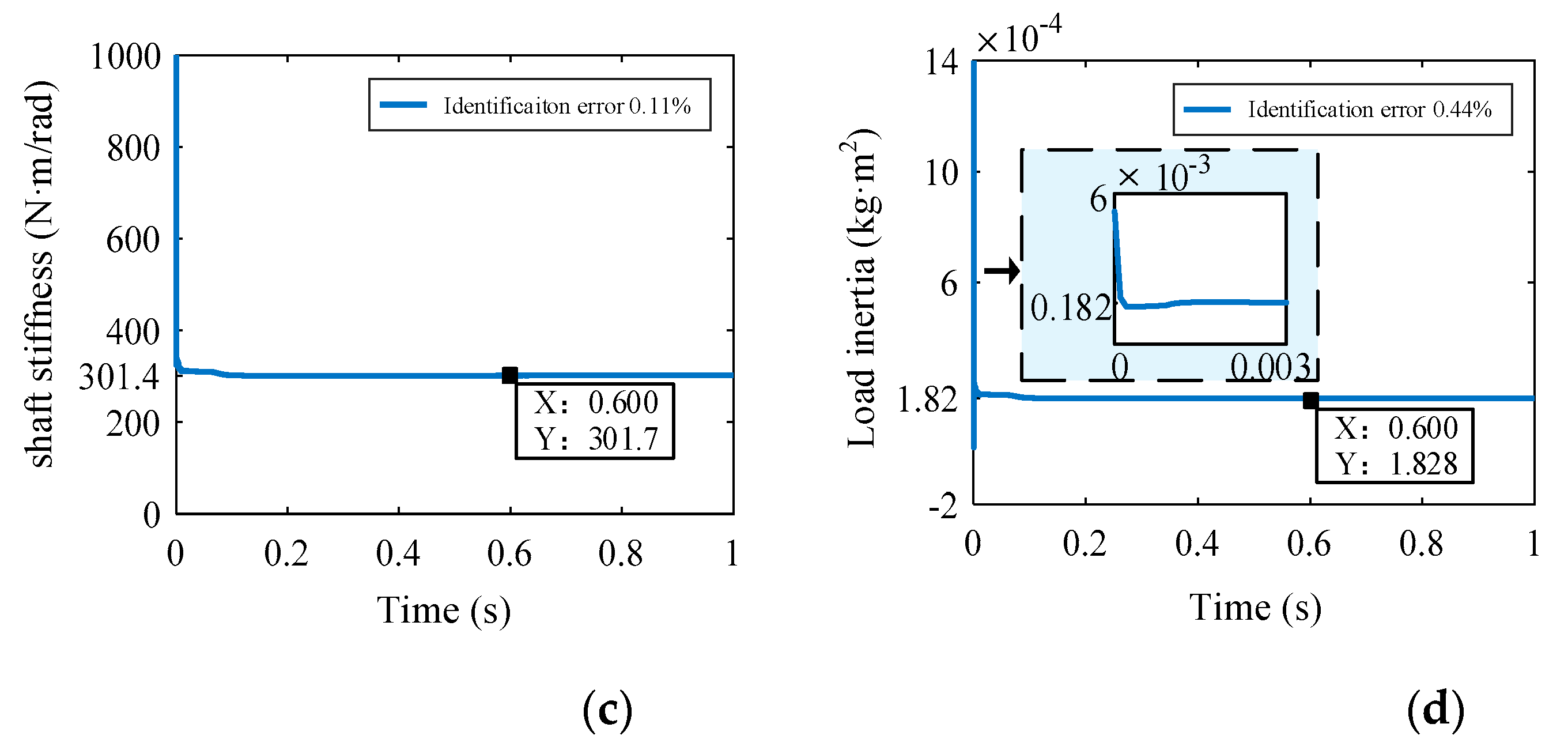
The rotational speed reference signal is n_r*=200+200sin(5πt) rpm, and the simulation sampling period is 0.0001s, and the identification results are shown in Figure 3 and Figure 4. The discrete domain parameter θ(4) converges from the initial value of 0.01 to the true value of 1 in (20), indicating the effectiveness of the current parameter identification algorithm. The comparison of the identification results with the actual values is shown in Table 2, with small identification errors and high identification accuracy.

5. Influence of System Parameters on Recognition Accuracy

(1) discrete time

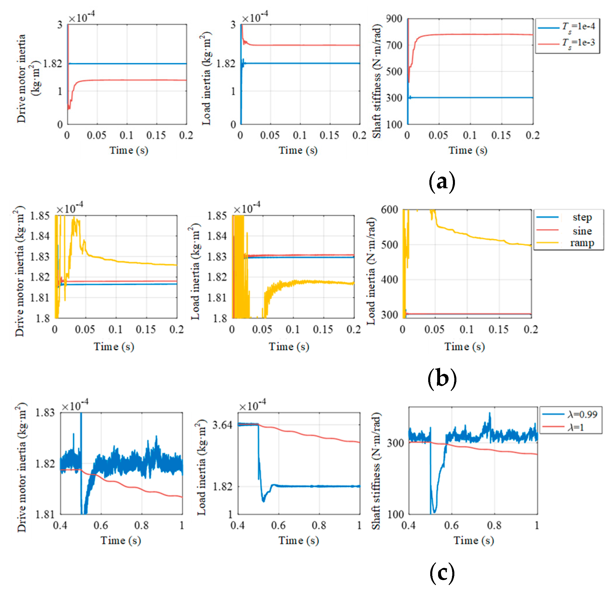
The smaller the discretization period is, the closer the discrete domain function is to the continuous domain function, and the higher the discrimination accuracy is [15]. Figure 5 (a) gives a comparison of the identification results in two cases where T_s is 0.001s and 0.0001s, respectively. When the discretization period is larger, the identification algorithm not only has a slow convergence process, but also has a poorer numerical accuracy in the final convergence.

(2) given signal

Given different speed signals, the comparison of the recognition results is shown in Table 2. Under the three signal forms, the recognition accuracies of the inertia J_m and J_l on both sides are high and can reach within 1% under ideal simulation conditions. However, the identification error of the shaft stiffness K under the slope given speed signal is extremely high, as high as 40.3%. As the slope of the given signal increases, the identification error decreases significantly. The simulation waveforms are shown in Figure 5(b) for the 2^nd, 4^th, and 6^th given signals. The convergence speeds and recognition accuracies of the step signal and sinusoidal signal do not differ much, but the convergence speeds are relatively slow and the recognition results fluctuate a lot in the slope given signal. From the derivation of the algorithm, it can be seen that the recognition process depends on the transient process of the motor speed rise, while the acceleration is small and the transient process is short when the ramp is given, which is not conducive to the recognition.

(3) forgetting factor

As mentioned before, the forgetting factor λ affects the convergence speed and volatility of the recognition results, and in the actual working condition, the work platform will have the situation of sudden load unloading, which leads to the sudden change of the load-side inertia, so it is necessary to carry out the relevant experiments to verify the robustness of the algorithm. Figure 5 shows the recognition waveforms under different forgetting factors when the load inertia is suddenly reduced at 0.5 s. When λ=1, the convergence is still not possible within 0.5 s, and the convergence speed is slow, but the waveform of the recognition result is smoother; when λ=0.99, the recognition result is re-converged to the vicinity of the true value within 0.1 s, and the convergence speed is fast, but there are many signal burrs and fluctuation is large.

Comprehensive consideration, this paper in the mechanical parameter identification experiment selected sinusoidal signal as a given signal, forgetting factor λ = 0.99, discretization time needs to be based on the performance of the controller and other algorithms to further determine the time required.

6. Experimental Verification

The iterative algorithm designed in section 3.3.2 is a fifth-order matrix operation, which takes more time, and FFRLS also has requirements for discrete time (i.e. sampling time), so it is necessary to test the algorithm time. The clock period of the controller used in the experiment is 0.67ns, and the running time of the test programmed using breakpoints is 4994 clock cycles (33μs) for the motor control programmed, and the time of the parameter recognition algorithm is shown in Table 4, with a total running time of 84μs for no-load operation, and 121μs for with-load operation When the current loop control frequency is 10kHz and the speed loop control frequency is 1kHz, the recognition time in the loaded case the discrimination time exceeds one current loop cycle. In order to simplify the control and improve the recognition accuracy as much as possible, the sampling time is 0.0002s.

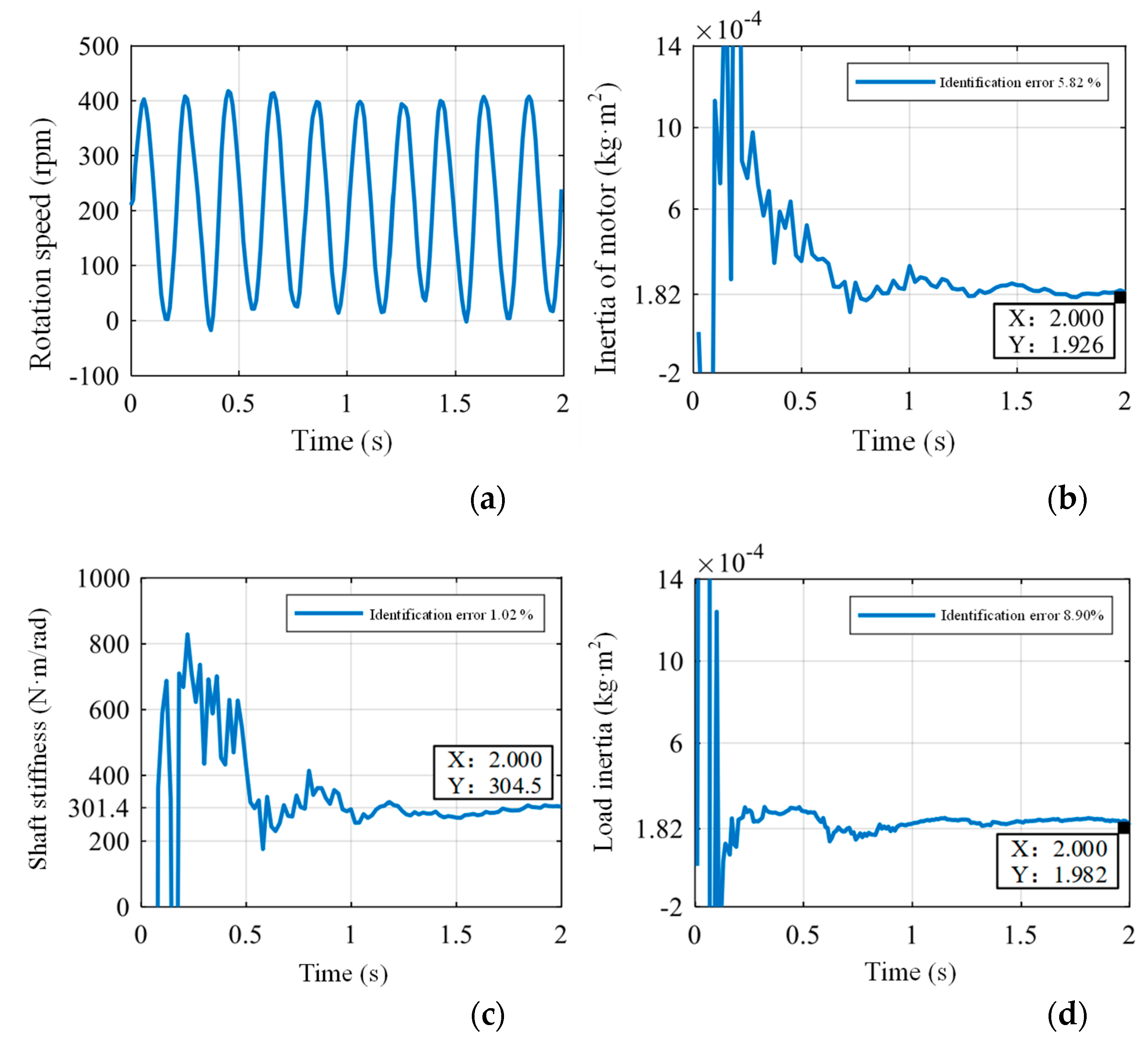
Given n_r*=200+200sin(5πt) rpm with sinusoidal speed, the system response waveform and the convergence waveform of the discriminated values of mechanical parameters are shown in Figure 6. It is considered to be basically converged in 0.6s, and the discriminated values of the drive motor inertia, load inertia, and shaft stiffness in 2s are 1.93×10^-4kg·m2, 1.98×10^-4kg·m2, and 304.5 N·m/rad, with identification errors of 5.82%, 8.90%, and 1.02%, respectively.

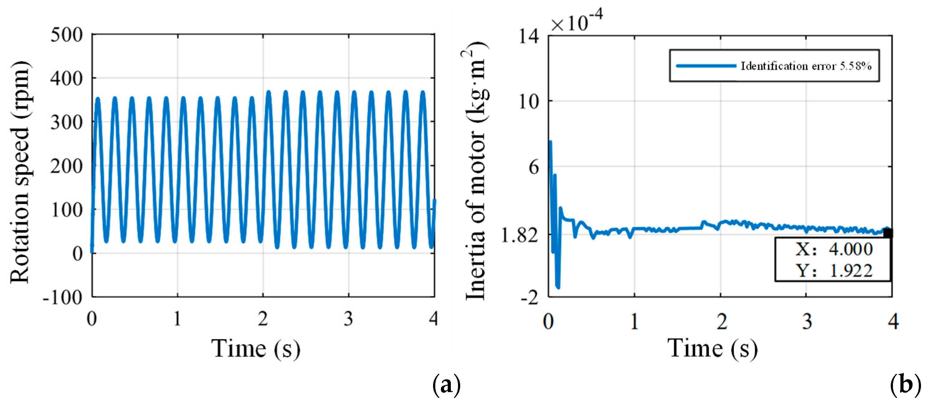
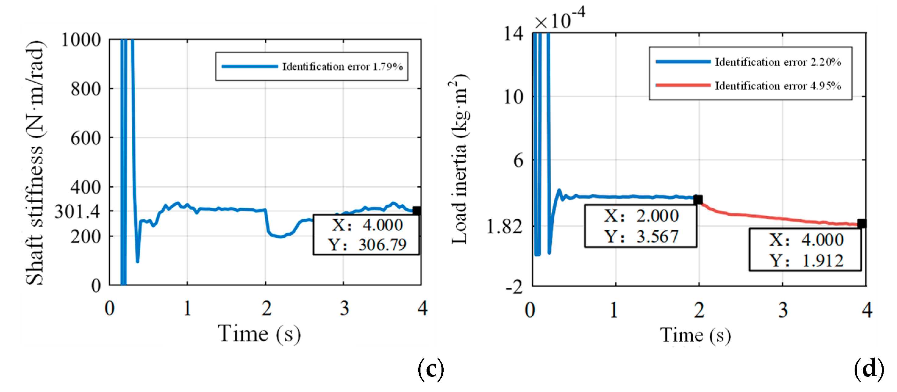
Figure 7 shows the system response and recognition waveforms when the load inertia changes suddenly. The load inertia decreases from 2J_l to J_l at 2s, the drive motor inertia and shaft stiffness converge to the real value after fluctuation, while the load inertia converges slower and the recognition accuracy decreases from 2.2% to 4.95%, which is due to the fact that the covariance matrix P is not re-initialized.

7. Conclusions

In this paper, to address the problem of unknown or inaccurate mechanical parameters, especially load-side inertia, in non-direct-drive servo systems, firstly, the system is simplified into a dual-inertia system, its equations of motion are analyzed and mathematically modelled. Secondly, using the least recursive squares method with forgetting factor, an online identification algorithm of the main mechanical parameters of the dual-inertia system is constructed to accurately obtain the dual-side inertia of the system and the stiffness of the coupling. The algorithm chooses the bilinear transformation discretization method, which avoids the computational solution of nonlinear equations and shortens the parameter conversion time of the algorithm. Finally, the proposed algorithm is simulated and experimentally verified, and the influencing factors of the recognition accuracy are discussed. The total time of the recognition algorithm under unloaded and loaded conditions is 51μs and 88μs respectively. The experiment shows that the mechanical parameter recognition algorithm of the dual-inertia system can simultaneously recognize the three main mechanical parameters online, and the recognition accuracy is high and has certain robustness.

References

Sul S, K. Control of Electric Machine Drive Systems; Wiley-IEEE Press: Piscataway, NJ, USA, 2011. [Google Scholar]
Zadeh, L.A. From Circuit Theory to System Theory. Proc. IRE 1962, 50, 856–865. [Google Scholar] [CrossRef]
Thenozhi, S.; Concha, A.; Resendiz, J.R. A Contraction Theory-based Tracking Control Design with Friction Identification and Compensation. IEEE Trans. Ind. Electron. 2022, 69, 6111–6120. [Google Scholar] [CrossRef]
Song, Z.; Mei, X.; Jiang, G. Inertia Identification based on Model Reference Adaptive System with Variable Gain for AC Servo Systems. In International Conference on Mechatronics and Automation (ICMA); IEEE: Takamatsu, Japan, 2017; pp. 188–192. [Google Scholar]
Lian, C.; Xiao, F.; Gao, S. , et al. Load Torque and Moment of Inertia Identification for Permanent Magnet Synchronous Motor Drives Based on Sliding Mode Observer. IEEE Trans. Power Electron. 2019, 34, 5675–5683. [Google Scholar] [CrossRef]
Perdomo, M.; Pacas, M.; Eutebach, T.; et al. Identification of Variable Mechanical Parameters Using Extended Kalman Filters. In International Symposium on Diagnostics for Electric Machines, Power Electronics and Drives (SDEMPED); IEEE: Valencia, Spain, 2013; pp. 377–383. [Google Scholar]
Andoh, F. Moment of Inertia Identification Using the Time Average of the Product of Torque Reference Input and Motor Position. IEEE Trans. Power Electron. 2007, 22, 2534–2542.1. [Google Scholar] [CrossRef]
Saarakkala, S.E.; Leppinen, T.; Hinkkanen, M.; et al. Parameter Estimation of Two-mass Mechanical Loads in Electric Drives. In International Workshop on Advanced Motion Control (AMC); IEEE: Sarajevo, Bosnia and Herzegovina, 2012; pp. 1–6.1. [Google Scholar]
Saarakkala, S.E.; Hinkkanen, M. Identification of Two-mass Mechanical Systems in Closed-loop Speed Control. In Annual Conference of the IEEE Industrial Electronics Society (IECON); IEEE: Vienna, Austria, 2013; pp. 2905–2910. [Google Scholar]
Luczak, D.; Nowopolski, K. Identification of Multi-mass Mechanical Systems in Electrical Drives. In Proceedings of the 16th International Conference on Mechatronics—Mechatronika; Brno, Czech Republic; 2014; pp. 275–282. [Google Scholar]
Zoubek, H.; Pacas, M. Encoderless Identification of Two-Mass-Systems Utilizing an Extended Speed Adaptive Observer Structure. IEEE Trans. Ind. Electron. 2016, 64, 595–604.1. [Google Scholar] [CrossRef]
Yoshioka, Y.; Hanamoto, T. Estimation of a Multimass System Using the LWTLS and a Coefficient Diagram for Vibration-Controller Design. IEEE Trans. Ind. Appl. 2008, 44, 566–574.1. [Google Scholar] [CrossRef]
Calvini, M.; Carpita, M.; Formentini, A. , et al. PSO-Based Self-Commissioning of Electrical Motor Drives. IEEE Trans. Ind. Electron. 2015, 62, 768–776.1. [Google Scholar] [CrossRef]
Gontrand, C. Digital Communication Techniques; Wiley-IEEE Press: Piscataway, NJ, USA, 2020. [Google Scholar]
Yang, M.; Qu, W.Y.; Chen, Y.Y. , et al. Online Inertia Identification of Servo Systems Based on Variable-period Recursive Least Squares and Kalman Observer. Journal of Electric Engineering, 2018, 33, 367–376. [Google Scholar]

Figure 1. Dual Inertia System Diagram

Figure 2. Simplified Block Diagram of Dual Inertia System

Figure 3. Convergence of parameter values in the discrete domain

Figure 4. Simulation results of mechanical parameter identification of dual-inertia system: (a) Motor speed waveform; (b) Drive motor inertia identification results; (c) Shaft stiffness identification results; (d) Load Inertia Recognition Results.

Figure 5. Analysis of factors affecting identification accuracy: (a) Different sampling times; (b) Different speed feed signal forms; (c) Different forgetting factors.

Figure 6. Experimental results of parameter identification of dual-inertia system. (a) Shaft stiffness identification results; (b) Load Inertia Recognition Results; (c) Shaft stiffness identification results; (d) Load inertia identification results.

Figure 7. Experimental results of parameter identification of dual-inertia system: (a) Shaft stiffness identification results; (b) Load Inertia Recognition Results;(c) Shaft stiffness identification results; (d) Load inertia identification results.

Table 1. Main parameters of the motor

Parameters	Value
Rated power (W)	750
Rated current (A)	3
Rated torque (N·m)	2.39
Poles	5
Inertia (kg·m²)	1.82×10^-4

Table 2. Simulation results of mechanical parameter identification of dual-inertia system

Parameters	Ture Value	Identification value	Identification Error (%)
J_m (kg·m²)	1.82×10^-4	1.813×10^-4	0.38
J_l (kg·m²)	1.82×10^-4	1.828×10^-4	0.44
K (N·m/rad)	301.36	301.7	0.11

Table 3. Parameter identification results for different speed givens.

No.	Given type	Value (rpm)	J_m identification error (%)	J_l IdentificationError (%)	K identification error (%)
1	Step	50	0.05	0.53	0.44
2	Step	200	0.29	0.44	0.59
3	ramp	1000t	0.38	0.06	40.3
4	ramp	4000t	0.42	0.20	6.85
5	sine	200sin(5πt)	0.05	0.57	0.46
6	sine	200sin(10πt)	0.16	0.37	0.49

Table 4. Dual Inertia System Parameter Identification Time Test

Load condition	Order of operation	Iteration duration	Conversion time	Total duration
Unladen	4	46μs	5μs	51μs
Payload	5	84μs	4μs	88μs

Disclaimer/Publisher’s Note: The statements, opinions and data contained in all publications are solely those of the individual author(s) and contributor(s) and not of MDPI and/or the editor(s). MDPI and/or the editor(s) disclaim responsibility for any injury to people or property resulting from any ideas, methods, instructions or products referred to in the content.

© 2024 by the authors. Licensee MDPI, Basel, Switzerland. This article is an open access article distributed under the terms and conditions of the Creative Commons Attribution (CC BY) license (http://creativecommons.org/licenses/by/4.0/).

Copyright: This open access article is published under a Creative Commons CC BY 4.0 license, which permit the free download, distribution, and reuse, provided that the author and preprint are cited in any reuse.

MDPI Initiatives

Important Links

Choose an area of interest and we will send you notifications of new preprints at your preferred frequency.

Disclaimer

An Online Identification Method for Mechanical Parameters of Dual-Inertia Servo System

Abstract

1. Introduction

2. Mathematical Modelling of Dual Inertia Systems

3. Identification of Mechanical Parameters for Dual Inertia Systems

3.1. The Principle of Least Squares

3.2. Mechanical Parameter Identification Algorithm for Dual-Inertia Systems

4. Simulation Verification

4.1. Algorithmic Validity

6. Experimental Verification

7. Conclusions

References

MDPI Initiatives

Important Links

Subscribe