Submitted:
15 June 2024
Posted:
17 June 2024
You are already at the latest version
Abstract
Keywords:
1. Introduction
- To increase the number of evaluations conducted on the original problem functions, thereby improving the fidelity of the surrogate models.
- To maintain the accuracy of the classification task achieved by the original model (eMODiTS).
- To analyze the surrogate model behavior compared with SAX-based discretization methods to verify whether the proposal maintains, improves, or worsens by incorporating these models regarding the well-known discretization approaches.
2. Materials and Methods
2.1. Symbolic Aggregate approXimation (SAX)
2.2. Multi-Objective Optimization Problem (MOOP)
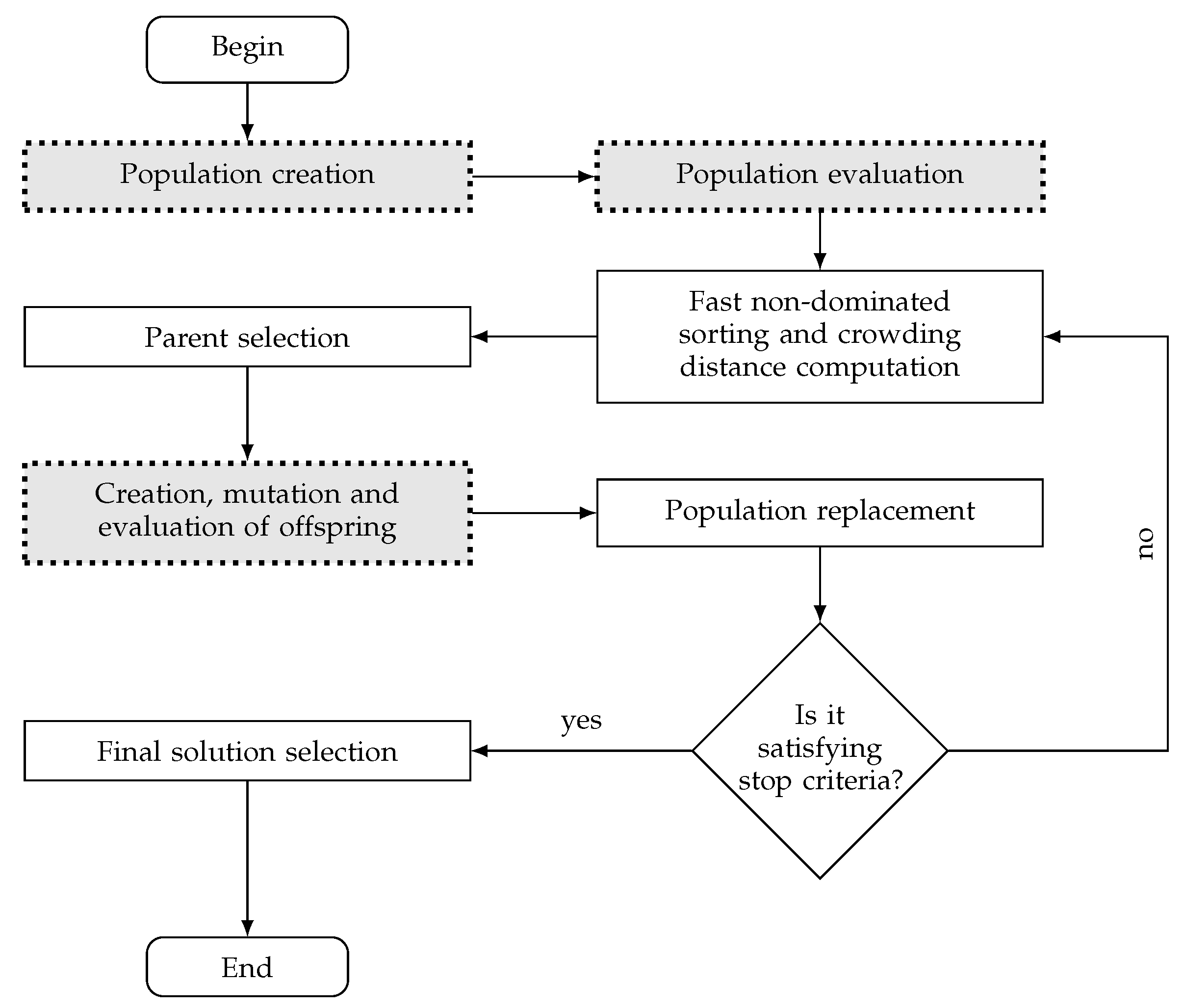
2.3. The Enhanced Multi-Objective Symbolic Discretization for Time Series (eMODiTS)
2.3.1. Population Generation
2.3.2. Evaluation Process
2.3.3. Offspring’s Creation and Mutation
2.3.4. Population Replacement
2.3.5. Preferences Handling
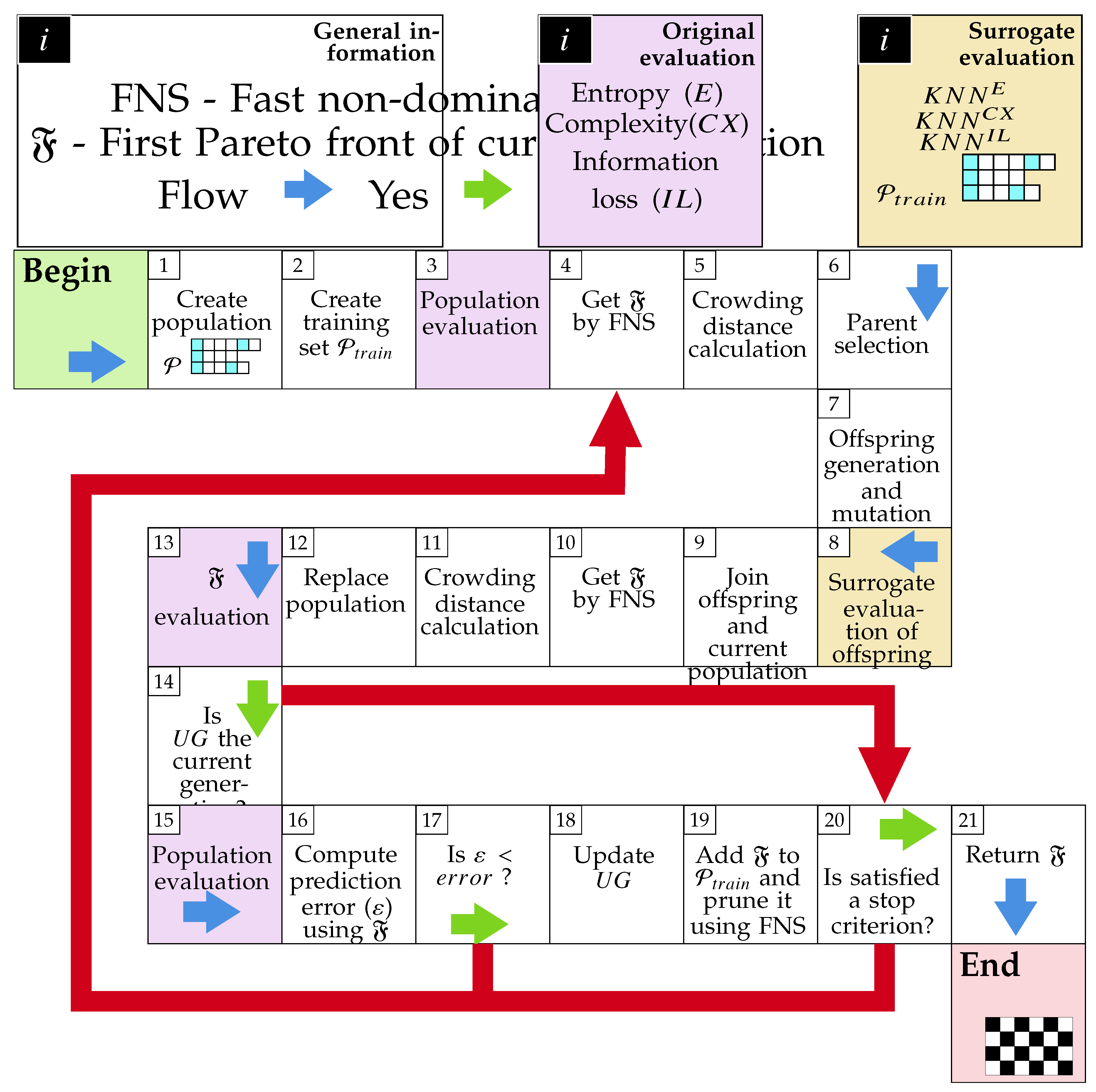
2.4. Surrogate-Assisted Multi-Objective Symbolic Discretization for Time Series (sMODiTS)
2.4.1. Training set creation
2.4.2. Surrogate model creation
2.4.3. Surrogate Model Update
2.5. Performance Metric for Surrogate Model Prediction
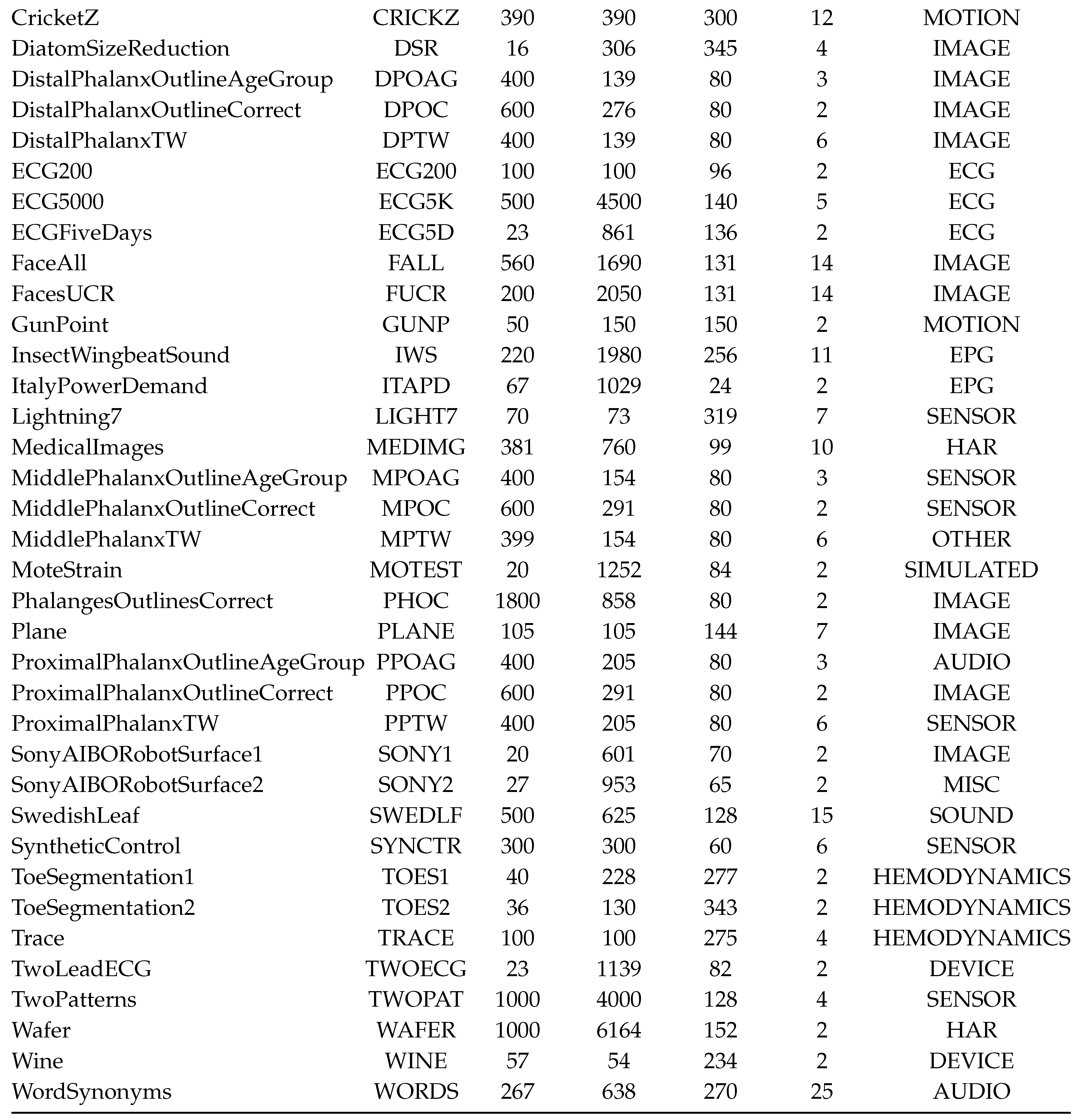
2.6. Datasets
3. Results and Discussion
3.1. Experimental Design
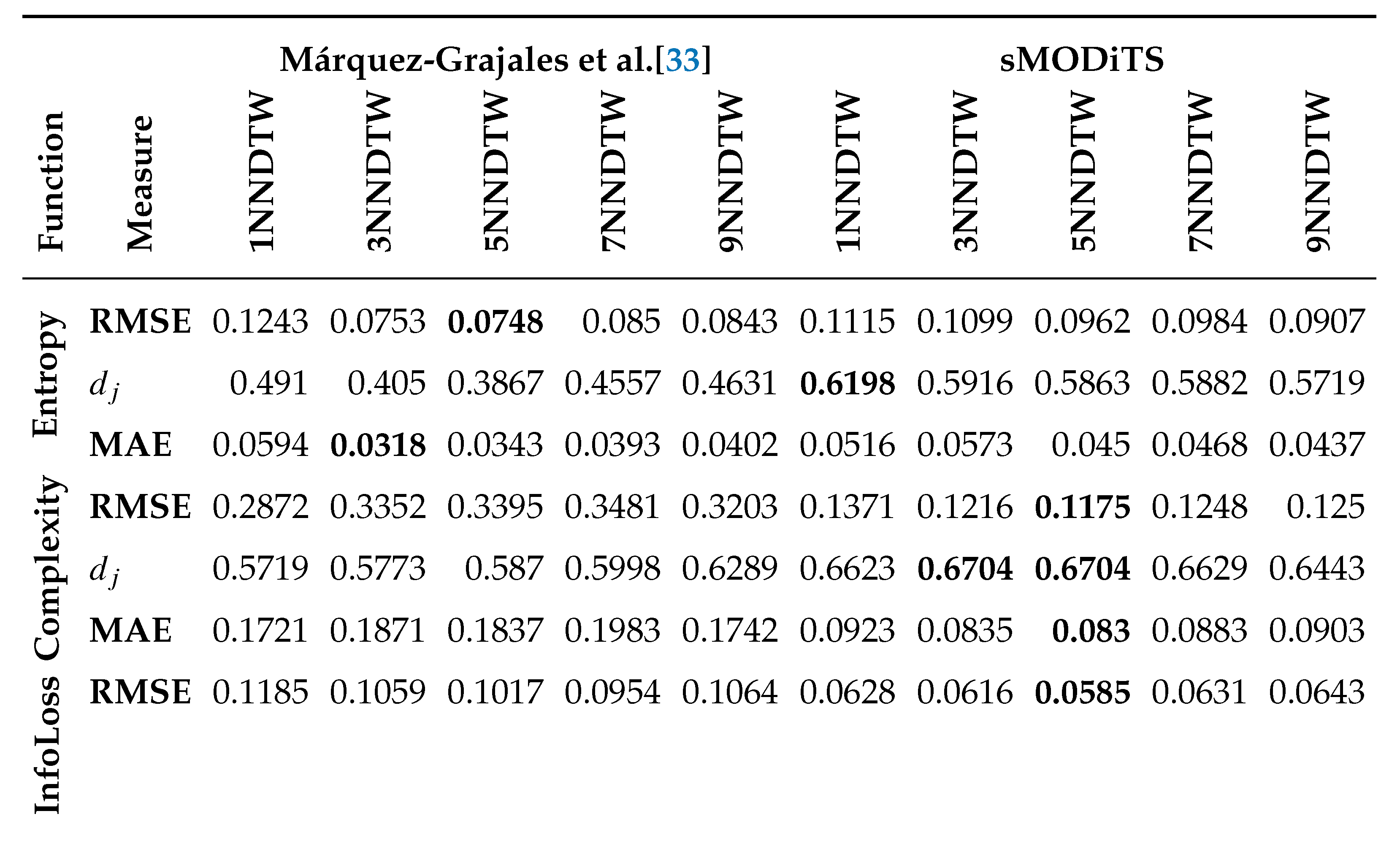
- Can sMODiTS increase the model fidelity regarding [33]? This question arises in analyzing the prediction power of sMODiTS and the proposal introduced in [33] compared to eMODiTS (original model). The results will seek to achieve the first research objective and are presented in Section 3.2.
- Is it possible to minimize the computational cost caused by evaluating the solutions in the eMODiTS functions without losing the ability to classify the time series? This question arises to achieve the second research objective, which seeks to find an alternative evaluation of the objective functions without losing the time series classification rate. The answer to this question will be presented in Section 3.3.
- Is sMODiTS a competitive alternative compared to SAX-based symbolic discretization models? Finally, this question arises to analyze whether implementing the surrogate models in sMODiTS remains competitive in the task for which the tool was designed. Therefore, a comparison is made against symbolic discretization models showing competitive performance in time-series classification. In Section 3.4, the results that answer this question will be presented.
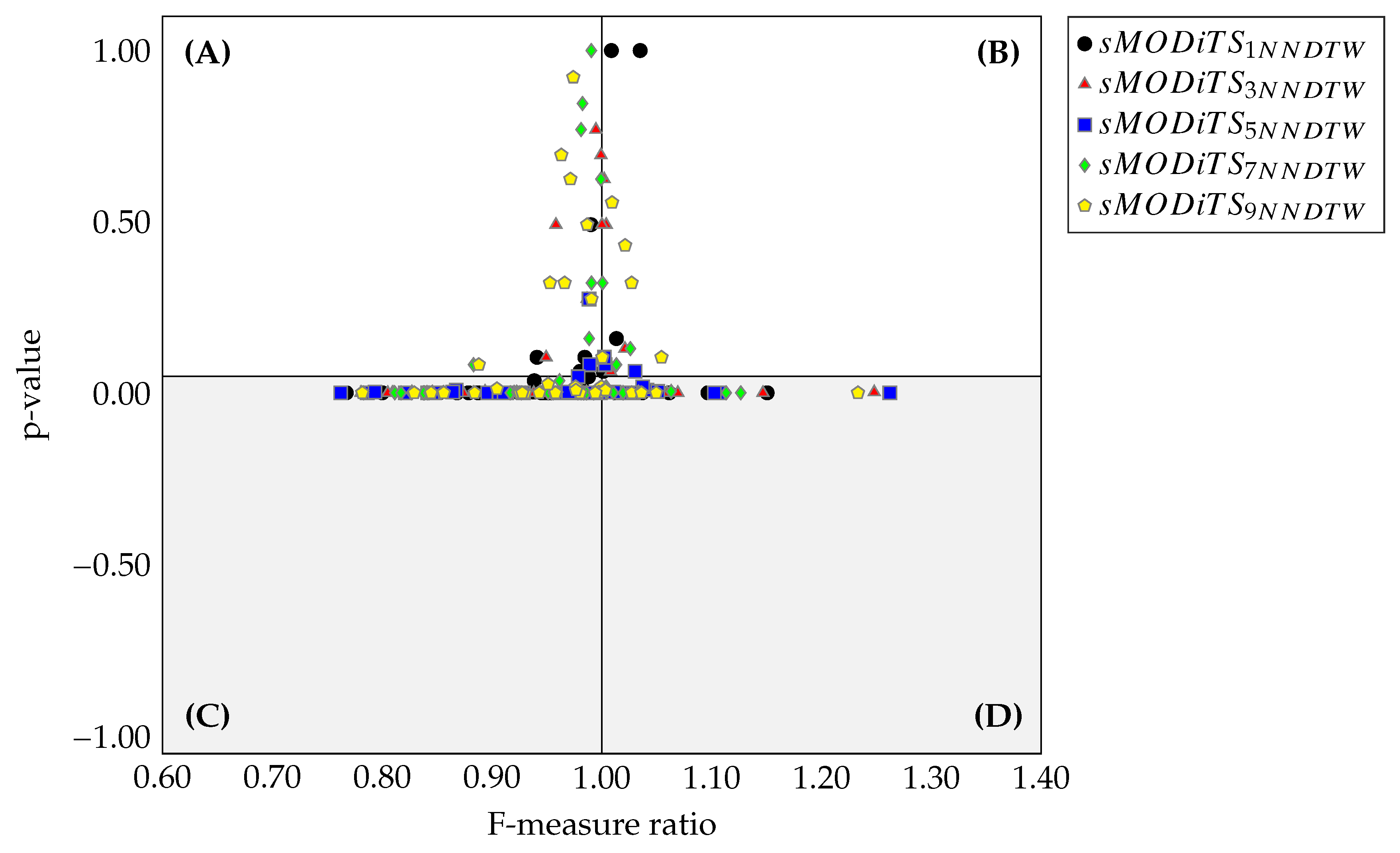
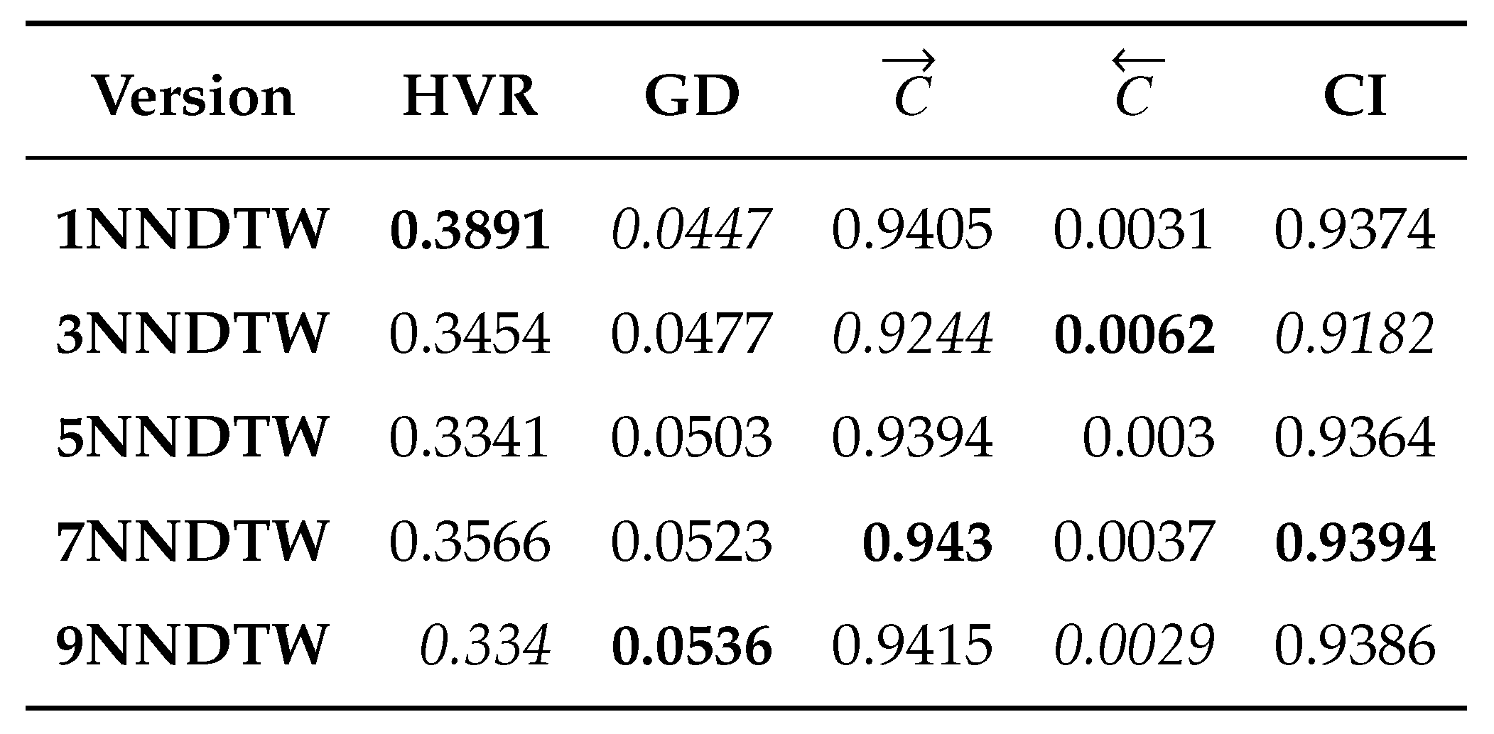
- Hypervolume Ratio (HVR) [34]. This metric is based on the hypervolume (H) measure, which computes the volume in the space of objective functions covered by a set of non-dominated solutions based on a reference point. Therefore, Equation 9 expressed the computation , where is the hypervolume of the obtained Pareto front and is the hypervolume of the true Pareto front. In this document, we take the True Pareto front the eMODiTS Pareto front and the obtained Pareto front the sMODiTS Pareto front. indicates that the sMODiTS Pareto front does not reach the eMODiTS Pareto front, indicates that both fronts are similar, and indicates that the sMODiTS Pareto front outperforms the eMODiTS Pareto front. Therefore, the ideal value is
- Generational Distance (GD) [77]. measures the closeness of the obtained and True Pareto front. Equation 10 shows this metric, where is the number of non-dominated solutions in the obtained Pareto front, and is the Euclidean distance between each solution of the obtained Pareto front and the nearest solution of the True Pareto front, measured in the space of the objective functions. Like HVR, for our purpose, the True Pareto front is taken as the eMODiTS Pareto front, and the obtained Pareto front is taken as the sMODiTS Pareto front. Values near zero indicate that the sMODiTS Pareto front is similar to the eMODiTS Pareto front.
- Coverage measure (C) [78]. This measure computes the fracción of two Pareto fronts covered or dominated by one another or vice versa. Equation 11 described this measure. represents that all elements of are dominated by the , otherwise indicates that no elements from are dominated by the . It is important to mention that and . Therefore, both scenarios must be analyzed to provide a wide panorama of this measure. Two Pareto fronts are considered similar when the coverage in both senses is zero simultaneously.
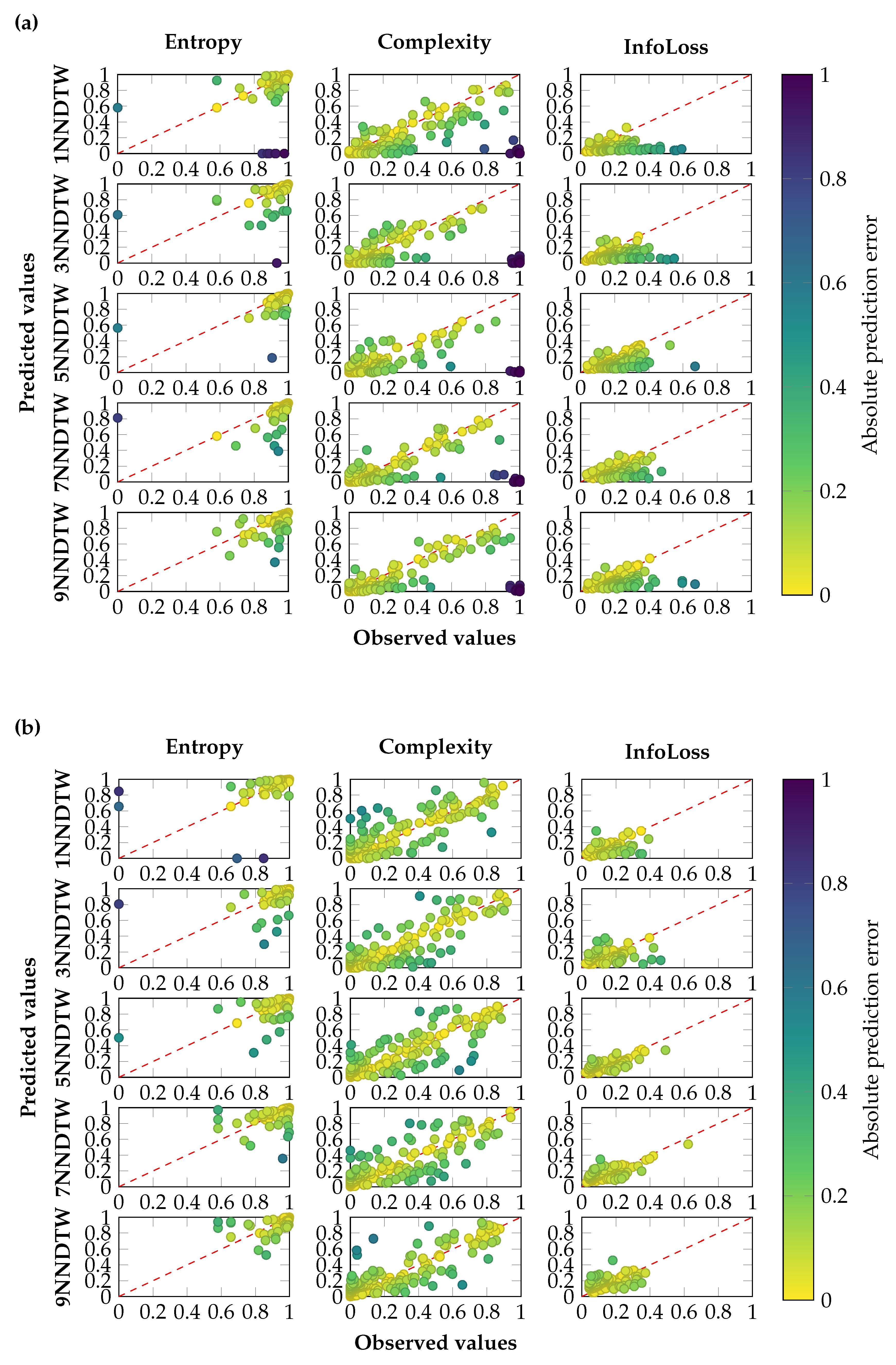
3.2. sMODiTS’ Prediction Power Analysis
3.3. Comparison between eMODiTS and sMODiTS
3.3.1. Classification Performance
3.3.2. Analysis of Pareto Fronts
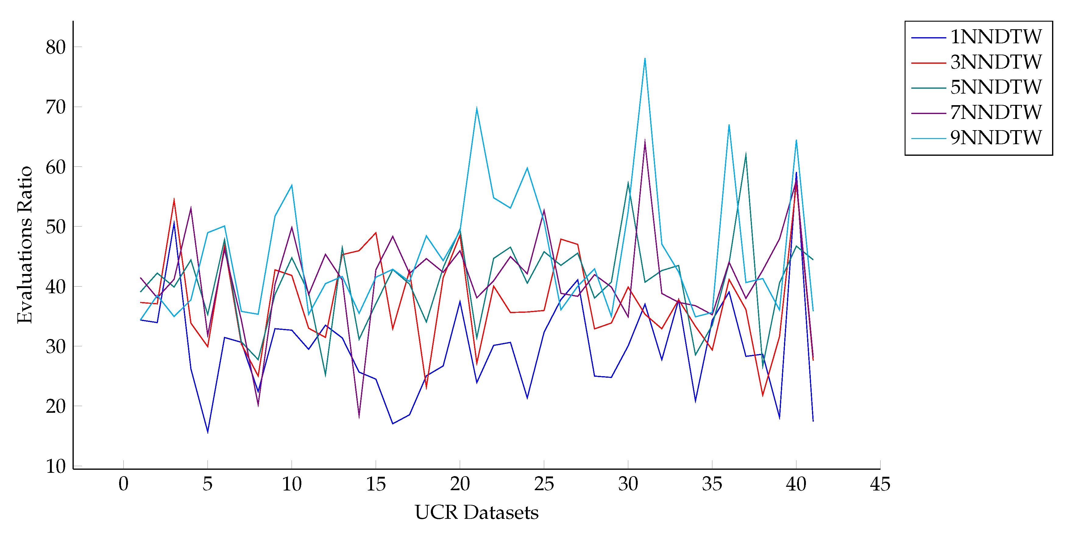
3.3.3. Computational Cost Analysis
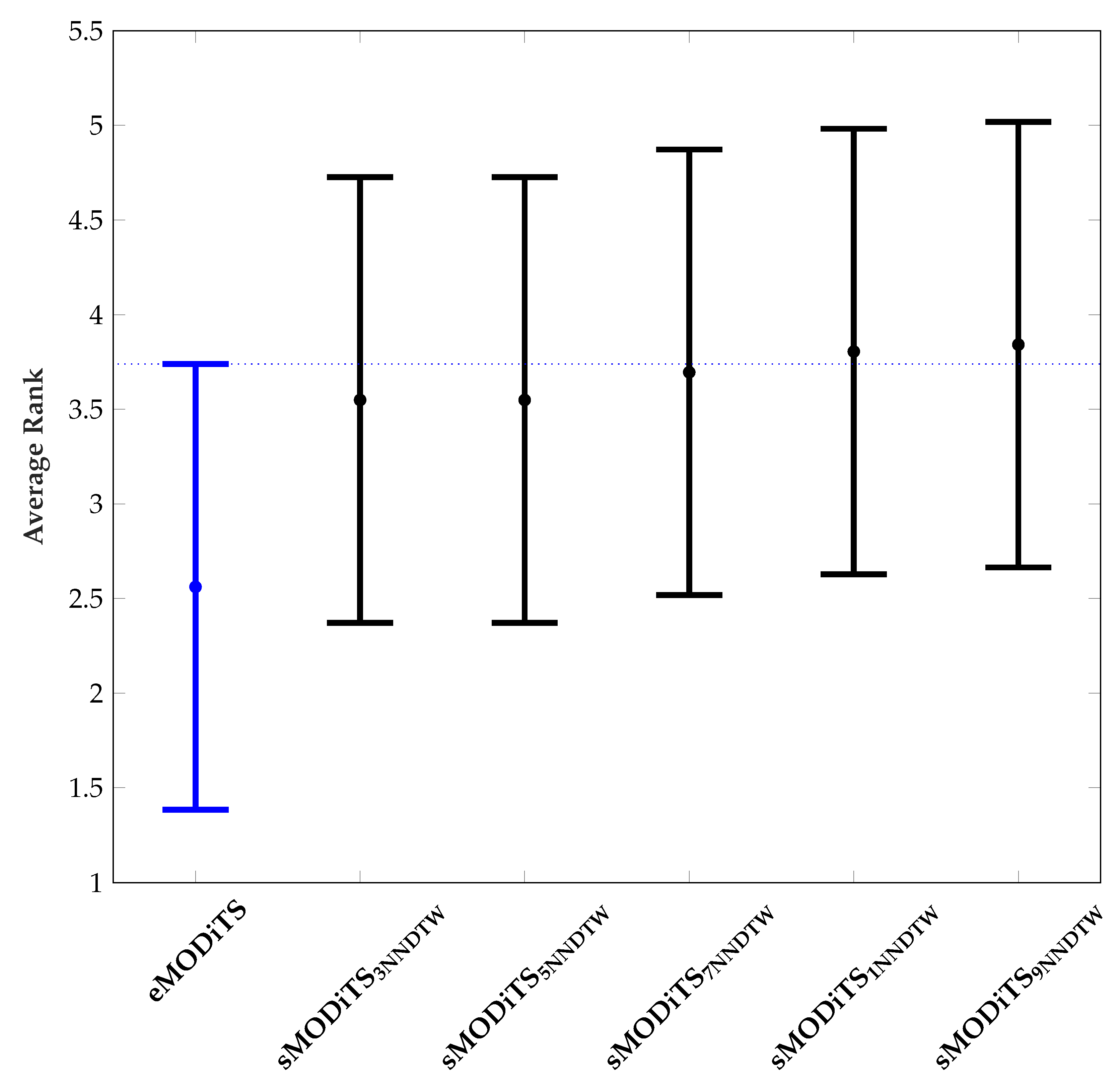
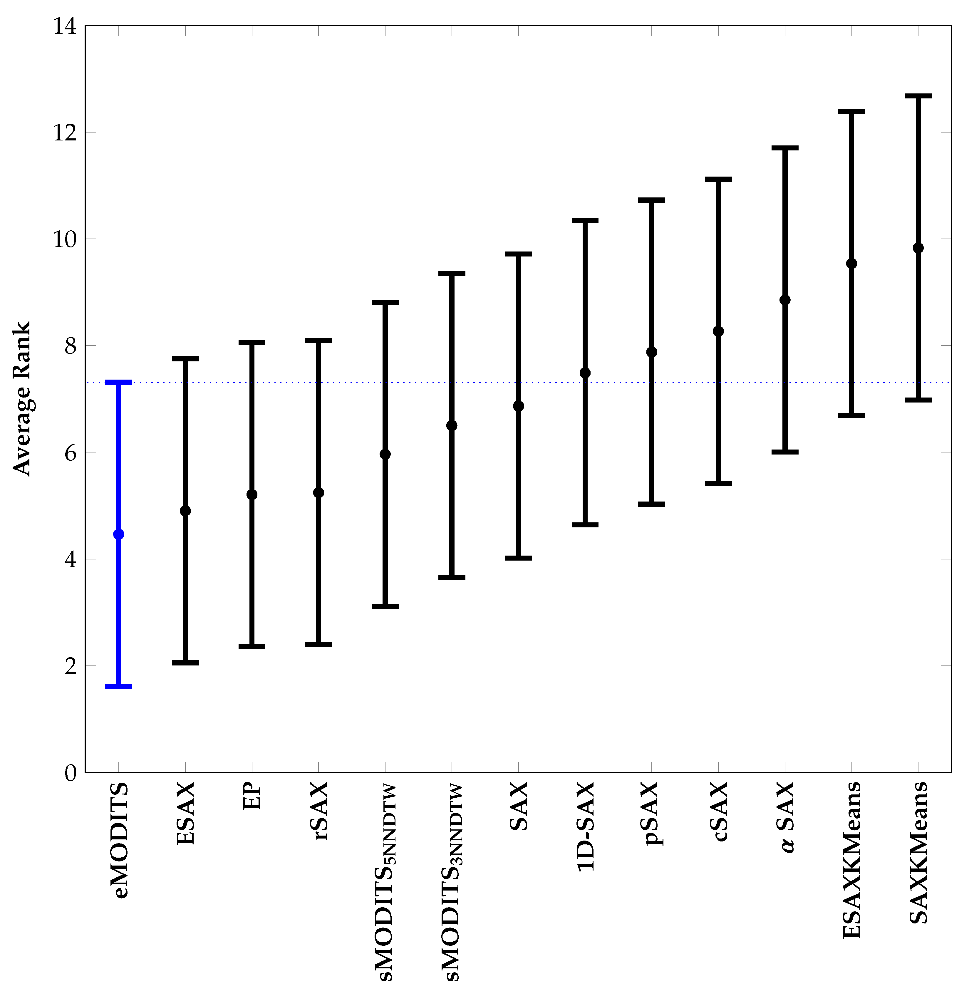
3.4. Comparison of sMODiTS among the SAX-Based Methods
4. Conclusions
Author Contributions
Data Availability Statement
Acknowledgments
Conflicts of Interest
References
- Dimitrova, E.S.; Licona, M.P.V.; McGee, J.; Laubenbacher, R. Discretization of time series data. Journal of Computational Biology 2010, 17, 853–868. [Google Scholar] [CrossRef] [PubMed]
- Lin, J.; Keogh, E.; Lonardi, S.; Chiu, B. A symbolic representation of time series, with implications for streaming algorithms. In Proceedings of the Proceedings of the 8th ACM SIGMOD workshop on Research issues in data mining and knowledge discovery, 2003, pp. 2–11.
- Lkhagva, B.; Suzuki, Y.; Kawagoe, K. Extended SAX: Extension of symbolic aggregate approximation for financial time series data representation. DEWS2006 4A-i8 2006, 7. [Google Scholar]
- Sant’Anna, A.; Wickström, N. Symbolization of time-series: An evaluation of sax, persist, and aca. In Proceedings of the 2011 4th international congress on image and signal processing. IEEE, 2011, Vol. 4, pp. 2223–2228.
- Zhang, H.; Dong, Y.; Xu, D. Entropy-based Symbolic Aggregate Approximation Representation Method for Time Series. In Proceedings of the 2020 IEEE 9th Joint International Information Technology and Artificial Intelligence Conference (ITAIC), 2020, Vol. 9, pp. 905–909. [CrossRef]
- Muhammad Fuad, M.M. Modifying the Symbolic Aggregate Approximation Method to Capture Segment Trend Information. In Proceedings of the Modeling Decisions for Artificial Intelligence; Torra, V.; Narukawa, Y.; Nin, J.; Agell, N., Eds., Cham, 2020; pp. 230–239.
- Hui, R.; Xiaoguang, H.; Jin, X.; Guofeng, Z. TrSAX—An improved time series symbolic representation for classification. ISA Transactions 2020, 100, 387–395. [Google Scholar] [CrossRef]
- Lkhagva, B.; Suzuki, Y.; Kawagoe, K. New time series data representation ESAX for financial applications. In Proceedings of the 22nd International Conference on Data Engineering Workshops (ICDEW’06). IEEE, 2006, pp. x115–x115.
- Pham, N.D.; Le, Q.L.; Dang, T.K. Two novel adaptive symbolic representations for similarity search in time series databases. In Proceedings of the 2010 12th International Asia-Pacific Web Conference. IEEE, 2010, pp. 181–187.
- Bai, X.; Xiong, Y.; Zhu, Y.; Zhu, H. Time series representation: a random shifting perspective. In Proceedings of the International Conference on Web-Age Information Management. Springer, 2013, pp. 37–50.
- Malinowski, S.; Guyet, T.; Quiniou, R.; Tavenard, R. 1d-sax: A novel symbolic representation for time series. In Proceedings of the International Symposium on Intelligent Data Analysis. Springer, 2013, pp. 273–284.
- He, Z.; Zhang, C.; Ma, X.; Liu, G. Hexadecimal Aggregate Approximation Representation and Classification of Time Series Data. Algorithms 2021, 14, 353. [Google Scholar] [CrossRef]
- Kegel, L.; Hartmann, C.; Thiele, M.; Lehner, W. Season-and Trend-aware Symbolic Approximation for Accurate and Efficient Time Series Matching. Datenbank-Spektrum 2021, 21, 225–236. [Google Scholar] [CrossRef]
- Bountrogiannis, K.; Tzagkarakis, G.; Tsakalides, P. Data-driven kernel-based probabilistic SAX for time series dimensionality reduction. In Proceedings of the 2020 28th European Signal Processing Conference (EUSIPCO). IEEE, 2021, pp. 2343–2347.
- Acosta-Mesa, H.G.; Rechy-Ramírez, F.; Mezura-Montes, E.; Cruz-Ramírez, N.; Jiménez, R.H. Application of time series discretization using evolutionary programming for classification of precancerous cervical lesions. Journal of biomedical informatics 2014, 49, 73–83. [Google Scholar] [CrossRef]
- Ahmed, A.M.; Bakar, A.A.; Hamdan, A.R. Harmony search algorithm for optimal word size in symbolic time series representation. In Proceedings of the 2011 3rd conference on data mining and optimization (DMO). IEEE, 2011, pp. 57–62.
- Ahmed, A.M.; Bakar, A.A.; Hamdan, A.R. A harmony search algorithm with multi-pitch adjustment rate for symbolic time series data representation. International Journal of Modern Education and Computer Science 2014, 6, 58. [Google Scholar] [CrossRef]
- Fuad, M.M.M. Differential evolution versus genetic algorithms: towards symbolic aggregate approximation of non-normalized time series. In Proceedings of the 16th International Database Engineering & Applications Sysmposium; IDEAS ’12; Association for Computing Machinery: New York, NY, USA, 2012; pp. 205–210. [Google Scholar] [CrossRef]
- Fuad, M.; Marwan, M. Genetic algorithms-based symbolic aggregate approximation. In Proceedings of the International Conference on Data Warehousing and Knowledge Discovery. Springer, 2012, pp. 105–116.
- Márquez-Grajales, A.; Acosta-Mesa, H.G.; Mezura-Montes, E.; Graff, M. A multi-breakpoints approach for symbolic discretization of time series. Knowledge and Information Systems 2020, 62, 2795–2834. [Google Scholar] [CrossRef]
- Jiang, P.; Zhou, Q.; Shao, X. Surrogate model-based engineering design and optimization; Springer, 2020.
- Koziel, S.; Pietrenko-Dabrowska, A. Rapid multi-criterial antenna optimization by means of pareto front triangulation and interpolative design predictors. IEEE Access 2021, 9, 35670–35680. [Google Scholar] [CrossRef]
- Koziel, S.; Pietrenko-Dabrowska, A. Rapid multi-objective optimization of antennas using nested kriging surrogates and single-fidelity EM simulation models. Engineering Computations 2020. [Google Scholar] [CrossRef]
- Koziel, S.; Pietrenko-Dabrowska, A. Fast multi-objective optimization of antenna structures by means of data-driven surrogates and dimensionality reduction. IEEE Access 2020, 8, 183300–183311. [Google Scholar] [CrossRef]
- Koziel, S.; Pietrenko-Dabrowska, A. Constrained multi-objective optimization of compact microwave circuits by design triangulation and pareto front interpolation. European Journal of Operational Research 2022, 299, 302–312. [Google Scholar] [CrossRef]
- Pietrenko-Dabrowska, A.; Koziel, S. Accelerated multiobjective design of miniaturized microwave components by means of nested kriging surrogates. International Journal of RF and Microwave Computer-Aided Engineering 2020, 30, e22124. [Google Scholar] [CrossRef]
- Amrit, A.; Leifsson, L.; Koziel, S. Fast multi-objective aerodynamic optimization using sequential domain patching and multifidelity models. Journal of Aircraft 2020, 57, 388–398. [Google Scholar] [CrossRef]
- Arias-Montano, A.; Coello, C.A.C.; Mezura-Montes, E. Mezura-Montes, E. Multi-objective airfoil shape optimization using a multiple-surrogate approach. In Proceedings of the 2012 IEEE Congress on Evolutionary Computation. IEEE, 2012, pp. 1–8.
- Fan, Y.; Lu, W.; Miao, T.; Li, J.; Lin, J. Multiobjective optimization of the groundwater exploitation layout in coastal areas based on multiple surrogate models. Environmental Science and Pollution Research 2020, 27, 19561–19576. [Google Scholar] [CrossRef]
- Dumont, V.; Garner, C.; Trivedi, A.; Jones, C.; Ganapati, V.; Mueller, J.; Perciano, T.; Kiran, M.; Day, M. HYPPO: A Surrogate-Based Multi-Level Parallelism Tool for Hyperparameter Optimization. In Proceedings of the 2021 IEEE/ACM Workshop on Machine Learning in High Performance Computing Environments (MLHPC), 2021, pp. 81–93. [CrossRef]
- Zheng Yi, W.; Atiqur, R. Optimized Deep Learning Framework for Water Distribution Data-Driven Modeling. Procedia Engineering 2017, 186, 261–268. [Google Scholar] [CrossRef]
- Vijayaprabakaran, K.; Sathiyamurthy, K. Neuroevolution based hierarchical activation function for long short-term model network. Journal of Ambient Intelligence and Humanized Computing 2021, 12, 10757–10768. [Google Scholar] [CrossRef]
- Márquez-Grajales, A.; Mezura-Montes, E.; Acosta-Mesa, H.G.; Salas-Martínez, F. Use of a Surrogate Model for Symbolic Discretization of Temporal Data Sets Through eMODiTS and a Training Set with Varying-Sized Instances. In Proceedings of the Advances in Computational Intelligence. MICAI 2023 International Workshops; Calvo, H.; Martínez-Villaseñor, L.; Ponce, H.; Zatarain Cabada, R.; Montes Rivera, M.; Mezura-Montes, E., Eds., Cham, 2024; pp. 360–372.
- Coello, C.A.C.; Lamont, G.B.; Veldhuizen, D.A.V. Evolutionary algorithms for solving multi-objective problems; Springer, 2007; Vol. 5. [Google Scholar]
- Rangaiah, G.P. Multi-objective optimization: techniques and applications in chemical engineering; Vol. 5, world scientific, 2016.
- Delboeuf, J. Mathematical psychics, an essay on the application of mathematics to the moral sciences, 1881.
- Deb, K.; Deb, K. Multi-objective Optimization. In Search Methodologies: Introductory Tutorials in Optimization and Decision Support Techniques; chapter 15; Springer: Boston, MA, USA, 2014; pp. 403–449. [Google Scholar] [CrossRef]
- Pareto, V. Cours d’économie politique; Vol. 1, Librairie Droz, 1964.
- Deb, K.; Agrawal, S.; Pratap, A.; Meyarivan, T. A fast elitist non-dominated sorting genetic algorithm for multi-objective optimization: NSGA-II. In Proceedings of the International conference on parallel problem solving from nature. Springer, 2000, pp. 849–858.
- Deb, K.; Pratap, A.; Agarwal, S.; Meyarivan, T. A fast and elitist multiobjective genetic algorithm: NSGA-II. IEEE transactions on evolutionary computation 2002, 6, 182–197. [Google Scholar] [CrossRef]
- Verma, S.; Pant, M.; Snasel, V. A comprehensive review on NSGA-II for multi-objective combinatorial optimization problems. Ieee Access 2021, 9, 57757–57791. [Google Scholar] [CrossRef]
- Syswerda, G.; et al. Uniform crossover in genetic algorithms. Proceedings of the ICGA, 1989; Vol. 3, 2–9. [Google Scholar]
- Poli, R.; Langdon, W.B. Genetic programming with one-point crossover. In Soft Computing in Engineering Design and Manufacturing; Springer, 1998; pp. 180–189.
- Mirjalili, S. Genetic algorithm. In Evolutionary algorithms and neural networks; Springer, 2019; pp. 43–55.
- Zainuddin, F.A.; Abd Samad, M.F.; Tunggal, D. A review of crossover methods and problem representation of genetic algorithm in recent engineering applications. International Journal of Advanced Science and Technology 2020, 29, 759–769. [Google Scholar]
- Singh, G.; Gupta, N. A Study of Crossover Operators in Genetic Algorithms. In Frontiers in Nature-Inspired Industrial Optimization; Springer, 2022; pp. 17–32.
- Singh, A.; Gupta, N.; Sinhal, A. Artificial bee colony algorithm with uniform mutation. In Proceedings of the Proceedings of the International Conference on Soft Computing for Problem Solving (SocProS 2011) December 20-22, 2011. Springer, 2012, pp. 503–511.
- Koziel, S.; Ciaurri, D.E.; Leifsson, L. Surrogate-based methods. In Computational optimization, methods and algorithms; Springer, 2011; pp. 33–59.
- Tong, H.; Huang, C.; Minku, L.L.; Yao, X. Surrogate models in evolutionary single-objective optimization: A new taxonomy and experimental study. Information Sciences 2021, 562, 414–437. [Google Scholar] [CrossRef]
- Miranda-Varela, M.E.; Mezura-Montes, E. Constraint-handling techniques in surrogate-assisted evolutionary optimization. An empirical study. Applied Soft Computing 2018, 73, 215–229. [Google Scholar] [CrossRef]
- Bhosekar, A.; Ierapetritou, M. Advances in surrogate based modeling, feasibility analysis, and optimization: A review. Computers & Chemical Engineering 2018, 108, 250–267. [Google Scholar]
- Fang, K.; Liu, M.Q.; Qin, H.; Zhou, Y.D. Theory and application of uniform experimental designs; Vol. 221, Springer, 2018.
- Kai-Tai, F.; Dennis K.J., L.; Peter, W.; Yong, Z. Uniform Design: Theory and Application. Technometrics 2000, 42, 237–248. [Google Scholar] [CrossRef]
- Yondo, R.; Andrés, E.; Valero, E. A review on design of experiments and surrogate models in aircraft real-time and many-query aerodynamic analyses. Progress in aerospace sciences 2018, 96, 23–61. [Google Scholar] [CrossRef]
- Díaz-Manríquez, A.; Toscano, G.; Barron-Zambrano, J.H.; Tello-Leal, E. A review of surrogate assisted multiobjective evolutionary algorithms. Computational intelligence and neuroscience 2016, 2016. [Google Scholar] [CrossRef]
- Deb, K.; Roy, P.C.; Hussein, R. Surrogate modeling approaches for multiobjective optimization: Methods, taxonomy, and results. Mathematical and Computational Applications 2020, 26, 5. [Google Scholar] [CrossRef]
- Lv, Z.; Wang, L.; Han, Z.; Zhao, J.; Wang, W. Surrogate-assisted particle swarm optimization algorithm with Pareto active learning for expensive multi-objective optimization. IEEE/CAA Journal of Automatica Sinica 2019, 6, 838–849. [Google Scholar] [CrossRef]
- Zhao, M.; Zhang, K.; Chen, G.; Zhao, X.; Yao, C.; Sun, H.; Huang, Z.; Yao, J. A surrogate-assisted multi-objective evolutionary algorithm with dimension-reduction for production optimization. Journal of Petroleum Science and Engineering 2020, 192, 107192. [Google Scholar] [CrossRef]
- Wang, X.; Jin, Y.; Schmitt, S.; Olhofer, M. An adaptive Bayesian approach to surrogate-assisted evolutionary multi-objective optimization. Information Sciences 2020, 519, 317–331. [Google Scholar] [CrossRef]
- Ruan, X.; Li, K.; Derbel, B.; Liefooghe, A. Surrogate assisted evolutionary algorithm for medium scale multi-objective optimisation problems. In Proceedings of the Proceedings of the 2020 genetic and evolutionary computation conference, 2020, pp. 560–568.
- Bao, K.; Fang, W.; Ding, Y. Adaptive Weighted Strategy Based Integrated Surrogate Models for Multiobjective Evolutionary Algorithm. Computational Intelligence and Neuroscience 2022, 2022. [Google Scholar] [CrossRef] [PubMed]
- Wang, X.; Jin, Y.; Schmitt, S.; Olhofer, M. Transfer Learning Based Co-Surrogate Assisted Evolutionary Bi-Objective Optimization for Objectives with Non-Uniform Evaluation Times. Evolutionary computation 2022, 30, 221–251. [Google Scholar] [CrossRef] [PubMed]
- Rosales-Pérez, A.; Coello, C.A.C.; Gonzalez, J.A.; Reyes-Garcia, C.A.; Escalante, H.J. A hybrid surrogate-based approach for evolutionary multi-objective optimization. In Proceedings of the 2013 IEEE Congress on Evolutionary Computation. IEEE, 2013, pp. 2548–2555.
- Bi, Y.; Xue, B.; Zhang, M. Instance Selection-Based Surrogate-Assisted Genetic Programming for Feature Learning in Image Classification. IEEE Transactions on Cybernetics 2021. [Google Scholar] [CrossRef] [PubMed]
- Blank, J.; Deb, K. GPSAF: A Generalized Probabilistic Surrogate-Assisted Framework for Constrained Single-and Multi-objective Optimization. arXiv 2022, arXiv:2204.04054 2022. [Google Scholar]
- Wu, M.; Wang, L.; Xu, J.; Wang, Z.; Hu, P.; Tang, H. Multiobjective ensemble surrogate-based optimization algorithm for groundwater optimization designs. Journal of Hydrology, 1281. [Google Scholar]
- Isaacs, A.; Ray, T.; Smith, W. An evolutionary algorithm with spatially distributed surrogates for multiobjective optimization. In Proceedings of the Australian Conference on Artificial Life. Springer, 2007, pp. 257–268.
- Datta, R.; Regis, R.G. A surrogate-assisted evolution strategy for constrained multi-objective optimization. Expert Systems with Applications 2016, 57, 270–284. [Google Scholar] [CrossRef]
- Kourakos, G.; Mantoglou, A. Development of a multi-objective optimization algorithm using surrogate models for coastal aquifer management. Journal of Hydrology 2013, 479, 13–23. [Google Scholar] [CrossRef]
- Yan, Y.; Zhang, Y.; Hu, W.; Guo, X.j.; Ma, C.; Wang, Z.a.; Zhang, Q. A multiobjective evolutionary optimization method based critical rainfall thresholds for debris flows initiation. Journal of Mountain Science 2020, 17, 1860–1873. [Google Scholar] [CrossRef]
- De Melo, M.C.; Santos, P.B.; Faustino, E.; Bastos-Filho, C.J.; Sodré, A.C. Computational Intelligence-Based Methodology for Antenna Development. IEEE Access 2021, 10, 1860–1870. [Google Scholar] [CrossRef]
- Gatopoulos, I.; Lepert, R.; Wiggers, A.; Mariani, G.; Tomczak, J. Evolutionary Algorithm with Non-parametric Surrogate Model for Tensor Program optimization. In Proceedings of the 2020 IEEE Congress on Evolutionary Computation (CEC). IEEE, 2020, pp. 1–8.
- Zhi, J.; Yong, Z.; Xian-fang, S.; Chunlin, H. A Surrogate-Assisted Ensemble Particle Swarm Optimizer for Feature Selection Problems. In Proceedings of the International Conference on Sensing and Imaging. Springer, 2022, pp. 160–166.
- Legates, D.R.; McCabe, G.J., Jr. Evaluating the use of “goodness-of-fit” Measures in hydrologic and hydroclimatic model validation. Water Resources Research 1999, 35, 233–241. [Google Scholar] [CrossRef]
- Keogh, E.e.a. The UCR Time Series Classification Archive, 2018. https://www.cs.ucr.edu/~eamonn/time_series_data_2018/.
- Ratanamahatana, C.A.; Keogh, E. Everything you know about dynamic time warping is wrong. In Proceedings of the Third workshop on mining temporal and sequential data. Citeseer, 2004, Vol. 32.
- Knowles, J.; Corne, D. On metrics for comparing nondominated sets. In Proceedings of the Proceedings of the 2002 Congress on Evolutionary Computation. CEC’02 (Cat. No.02TH8600), 2002, Vol. 1, pp. 711–716 vol.1. [CrossRef]
- Ascia, G.; Catania, V.; Palesi, M. A GA-based design space exploration framework for parameterized system-on-a-chip platforms. IEEE Transactions on Evolutionary Computation 2004, 8, 329–346. [Google Scholar] [CrossRef]



| Parameter | Value |
|---|---|
| Population size | 100 |
| Generation number | 300 |
| Independent executions number | 15 |
| Crossover rate | 80% |
| Mutation rate | 20% |

Disclaimer/Publisher’s Note: The statements, opinions and data contained in all publications are solely those of the individual author(s) and contributor(s) and not of MDPI and/or the editor(s). MDPI and/or the editor(s) disclaim responsibility for any injury to people or property resulting from any ideas, methods, instructions or products referred to in the content. |
© 2024 by the authors. Licensee MDPI, Basel, Switzerland. This article is an open access article distributed under the terms and conditions of the Creative Commons Attribution (CC BY) license (http://creativecommons.org/licenses/by/4.0/).


