Establishment and Application of Recursive Digital Processing Algorithm with Difference Analysis-Based Parameter Setting and Difference Feedback

Tongnan Xia; Bei Wang; Enruo Huang; Hong Jiang; Laiwu Zhang; Ming Liu; Chin-Chen Chang; Yaojie Sun

doi:10.20944/preprints202406.1307.v1

Preprint

Article

Establishment and Application of Recursive Digital Processing Algorithm with Difference Analysis-Based Parameter Setting and Difference Feedback

This version is not peer-reviewed.

Tongnan Xia

Bei Wang,Enruo Huang,

Ming Liu^*,

Bei Wang,Enruo Huang,

Ming Liu^*,

This version is not peer-reviewed.

Downloads

Views

Comments

Submitted:

18 June 2024

Posted:

19 June 2024

You are already at the latest version

A peer-reviewed article of this preprint also exists.

Abstract

Signal preprocessing and feature extraction are two important and necessary steps of data analysis. In signal analysis, typically these two steps are implemented through multiple algorithms. Moreover, the significant parameters in most algorithms are set empirically. We have developed an algorithm that can preserve and highlight characteristic waveforms while attenuating non-feature waveforms. The parameters in the algorithm are set through difference analysis. We have conducted experiments on both clinical and open-source ECG data, obtaining effective test results.

Keywords:

Algorithm Model

;

Signal Processing

;

Signal Smoothing

;

Feature Localization

Subject:

Computer Science and Mathematics - Computational Mathematics

1. Introduction

In signal processing, preprocessing and feature extraction are two indispensable steps[1,2]. In methods analyzing signals based on data collected by analytical instruments, data preprocessing is a crucial step[3]. Data preprocessing not only enhances the accuracy of subsequent analysis results but also improves the efficiency of data processing[4]. To achieve effectively signal preprocessing for further data analysis, scholars have employed various methods. The methods for preprocessing mainly include various types of digital filters (high-pass filters[5], low-pass filters[6], band-pass filters[7], notch filters[8], etc.), adaptive filters[9], wavelet transforms[10], Empirical Mode Decomposition[11], methods based on neural networks[12], and machine learning algorithms[13,14]. Feature extraction is a crucial step in the analysis of medical signals[15]. Since biomedical signals typically contain a large amount of raw data, feature extraction can transform the data into representative features, reducing data dimensionality, thus to simplify subsequent analysis processes. It also aids in identifying and extracting key information and patterns from signals, helping reveal underlying physiological or pathological characteristics embedded in the signal. Feature extraction is primarily achieved by extracting features from the time domain[16], frequency domain[17], time-frequency domain[18], decomposition domain[19], and deep features using filters with different functions[20].

However, in most studies, common to establish at least two algorithm models to achieve the aforementioned two goals. Currently, it remains further research and development to use the same algorithm to highlight feature areas as well as smooth non-feature areas that are seemingly contradictory functions.

This study explored the possibility of using the same algorithm to highlight feature areas while smoothing non-feature areas, and established an algorithm model with a sign difference feedback system based on statistical analysis. As shown in Figure 1.

2. Method

2.1. Mathematical Formulation of the Algorithm

For digital signal processing systems, the input of the system is a one-dimensional image, and a one-dimensional image can be abstracted as a binary function, denoted as

f (x, y)

. Here,

(x, y)

represents the pixel position, and

f (x, y)

represents the signal intensity at that position. After passing through an image processing system, the output is still a function. Therefore, image processing is essentially an operation on a function. The input to this processing system is a binary function, and the output is also a binary function.

The spatial domain method involves direct operations on pixels in an image. If we denote the output function as

g (x, y)

, at position

(x, y)

, the value of

g (x, y)

is highly correlated with the pixels at the corresponding position in the input image and its neighborhood. The mathematical model for the spatial domain method is shown in Equation (1).

Research manuscripts reporting large datasets that are deposited in a publicly available database should specify where the data have been deposited and provide the relevant accession numbers. If the accession numbers have not yet been obtained at the time of submission, please state that they will be provided during review. They must be provided prior to publication.

Interventionary studies involving animals or humans, and other studies that require ethical approval, must list the authority that provided approval and the corresponding ethical approval code.

g (x, y) = T [f (x, y)],

(1)

In Equation (1), T: a signal processing system,

(x, y)

: the pixel position,

f (x, y)

: the signal intensity at position (x, y) (the magnitude of the input),

g (x, y)

: the signal output intensity at position

(x, y)

For a signal with the following characteristics: continuous gradient ascent and descent segments are considered as valid signals or feature-extracted signals; sporadic or short-duration gradient ascent and descent segments are considered as interference signals or non-feature signals; non-feature extraction signals may exhibit directional interference. It is required that the output signal retains the trend and amplitude of the feature-extracted signal, preserving the shape corresponding to the raw signal. The algorithm model we have established addresses the above issues, as shown in Equation (2).

d_{n} = \{\begin{matrix} y_{1}, n = 1 \\ (\sum_{i = 1}^{n - 1} α \cdot {| ∆ y}_{n - i} |) + |∆ y_{n}|, n \geq 2 \\ ∆ y_{i} = \frac{y_{i} - y_{i - 1}}{x_{i} - x_{i - 1}}, i \geq 2 \\ ∆ y_{1} = y_{1} \end{matrix},

(2)

In Equation (2),

y_{i}

: the amplitude of the

i

th input signal,

x_{i}

: the index of the

i

th input signal,

d_{i}

: the amplitude of the

i

th output signal,

α

: a weight power,

α ϵ (0.9,1)

2.2. Meaning and Purpose

To facilitate the explanation of the meaning and purpose of the algorithm, we present Equation (2) in a logical form, as shown in Equation (3).

Y = y_{1} + y_{2},

(3)

In the Equation (3),

Y

：

d_{n}

，

y_{1}

：

\sum_{i = 1}^{n - 1} α \cdot {| ∆ y}_{n - i} |

，

y_{2}

：

|∆ y_{n}|

We view the output function of Equation (2) as a superposition of two function results. One is the function

y_{1}

, and the other is the function

y_{2}

. The discrete form of function

y_{1}

is shown in Equation (4).

y_{1 i} = {α \cdot d}_{i - 1}, i \geq 2,

(4)

In Equation (4),

y_{1 i}

: the value of the

i

th output signal,

α

: the weight power,

α ϵ [0,1]

In Equation (4), corresponding to function

y_{1}

, the operation involves self-repetition, indicating a recursive algorithm based on the recursive principle. It influences the current output based on the previous output, and when

0 < α < 1

, the signal is attenuated. Since the output is a part of the previous output, when the signal undergoes significant changes in adjacent time periods, the output signal remains relatively smooth. When

α

approaches 1, the smoothing effect of the filter becomes more pronounced. With

α

closer to 1, the signal changes more smoothly as it depends more on the previous output. A larger

α

value can better suppress signal fluctuations, reduce the impact of noise, and stabilize the signal. When

α

is a fixed value, meaning the output is a fixed proportion of the previous output, it implies that the current output is a part of the previous output, and the proportion is fixed. This helps reduce signal fluctuations and noise. Therefore, in Equation (2), we provide a more effective range for

α

The discrete form of

y_{2}

is shown in Equation (5).

y_{2 i} = {| d a t a}_{i} - {d a t a}_{i - 1} |,

(5)

y_{2 i}

：The

i

th predicted value，

{d a t a}_{i}

：The

i

th actual observed value.

Equation (5), which represents function

y_{2}

, is used to maintain the continuous trend. When the input prediction signal exhibits continuous changes, whether ascending or descending, Equation (5) reflects this change, which is added to the output sequence. This ensures that the output signal maintains consistency with the continuous trend of the input signal. If the input signal is continuously increasing, the output sequence will also continue to rise. Due to the influence of the first part of the function

y_{1}

, the output sequence smoothly follows the overall trend of the input signal, while the function

y_{2}

part retains the trend of the input signal. Therefore, if the input signal is continuously decreasing, the output sequence will also continue to decrease. The waveform shape of the output aligns with the waveform shape of the input signal, which is the result of the combined effects of both

y_{1}

and

y_{2}

components.

2.3. Parameter Settings based on Difference Analysis

Parameter settings are crucial for the algorithm model. In this study, we further determined the value of the weight constant

α

based on the empirical range of the smoothing filter algorithm weight constant and the design of each part of this algorithm model, using the method of difference testing analysis.

The purpose of the algorithm model established in this study is to preserve the main features of valid signals while smoothing and attenuating noise and interference signals, thereby highlighting the primary characteristics of the observations and reducing the amplitude of noise signals. Therefore, when setting parameters, we need to consider both aspects, aiming to reduce interference signals without affecting the main feature signals. Based on the above analysis, we provide the train of thought for parameter settings, as shown in Figure 2.

As shown in Figure 2, our algorithm serves two purposes simultaneously: preserving the trend of the raw data and reducing noise, smoothing the data to minimize interference with subsequent signal processing. Therefore, for signals with small amplitude fluctuations, smoothing and noise reduction are necessary, while the shape of the main feature signals needs to be retained. The setting of the parameter α plays a crucial role in achieving these two objectives. In various existing preprocessing algorithms, parameter settings are often based on empirical values. In contrast to previous studies, we determine the parameter

α

using a method based on statistical difference analysis to enhance the stability and adaptability of the model.

By conducting difference testing between the observed (raw) data and the predicted (output after model processing) data, we obtain the differences between the two sets of data. In statistics, if the p (Significance) of the two datasets is not less than 0.05, it is considered that their difference is not significant. In the context of our algorithm’s functionality, this indicates that the trend of the main data features has been preserved, confirming a successful setting for

α

. For datasets where the differences are significant, it is due to the changes in non-feature signal segments after weakening, leading to a significant difference in the analysis. To avoid the interference of these signal segments on parameter setting, we need to perform a regression setting on these signals. Subsequently, based on difference analysis, we reset the parameter α by setting these signals to the corresponding data values after filtering, reducing their impact on the setting of

α

. This process is iterated by refining the observed data and predicted data through difference testing, adjusting the value of

α

with an accuracy of 0.01 until the p satisfies the statistical condition (p>=0.05), thus achieving the setting for parameter

α

As a decay factor, the parameter

α

typically ranges between (0,1). When

α \to 0

, the absolute difference between the current data point and the previous data point contributes less to the result, indicating a smoother model that focuses more on past data. Conversely, as

α \to 1

, the model becomes more flexible, placing greater emphasis on recent changes. For algorithm models requiring both fast responsiveness to data and high stability, or when the data itself exhibits a high degree of autocorrelation, higher

α

values can better capture the dynamic characteristics of the data. Here, we limit

α

to the range between (0.9, 1), with an accuracy of 0.01. This ensures that the model can react strongly to changes in the most recent data points without overly relying on them, while still retaining some influence from historical data. This approach helps maintain relative stability when processing rapidly changing data, striking a better balance between the weight of historical and recent data.

Based on the analysis above, we need to preliminarily set

α

within this range. In this study, we set

α

to 0.94 initially. We then conduct a difference test between the observed and predicted values using this preset

α

. The steps for the difference test are outlined in Figure 3. Since the observed values (raw data) and predicted values (model output data) are paired samples, we need to use a paired sample test to examine the differences between these two sets of data. By calculating the differences between the observed and predicted values and denoting them as d, we assess whether d follows a normal distribution. As d does not exhibit normal distribution characteristics, we use a paired sample Wilcoxon test to compare the two sets of data.

We observe the p of the test result to determine if it is greater than 0.05. If the p is greater than 0.05, it indicates that our parameter setting has been successful. This means that we have effectively smoothed out interference segments with noise and fluctuations while preserving the original feature signals. If the p is not greater than 0.05, it is likely due to changes in the interference signals affecting the test results. In such a case, normalization of the observed data is required.

This involves two steps: Resetting negative values in the observed data. Since the output signal from the algorithm model has already removed sign interference, negative values in the predicted data are set to the corresponding data values in the output signal. Resetting signals near the equilibrium position in the observed data, such as signals close to the zero line, to the corresponding predicted values. This helps reduce the impact of differences caused by the smoothing of signals near the equilibrium position after model processing.

Finally, the reset observed signals are paired with the original predicted signals for a paired sample Wilcoxon test. We iteratively adjust the value of

α

with an accuracy of 0.01 until the p is greater than 0.05. At this point, the current

α

value is selected as the coefficient for the algorithm, indicating a successful parameter setting.

Taking a single clinical ECG data sample from Lead II with a sampling frequency of 500Hz and a duration of 10 seconds as the observed data

d_{1}

, sourced from Zhongshan Hospital affiliated to Fudan University using the Inno-12-U ECG device), we illustrate the difference testing based on the parameter settings. Initially, we set

α = 0.94

as a preset value. Subsequently, after running the algorithm model, we obtain the predicted values

y_{1}

. We calculate the difference d between

d_{1}

and

y_{1}

, and perform a normality test on data d. The results are shown in Table 1, where the significance Sig. (value p) = 0.000 < 0.05, indicating that data d is non-normally distributed.

Since the data is non-normally distributed, we need to perform a paired sample Wilcoxon test on the two sets of data,

d_{1}

and

y_{1}

. The test results are shown in Table 2. As the significance Sig. (value p) = .000 < 0.05 of the test results for both sets of data, it indicates that

y_{1}

has undergone significant changes due to smoothing and noise reduction, resulting in a significant difference between

y_{1}

and

d_{1}

At this point, we cannot determine if the value of the parameter

α

meets the requirement to preserve the main features and trends of

d_{1}

. Therefore, we need to reset

d_{1}

. In this example, due to significant differences in the amplitude of the characteristic waveforms in the ECG data, we first set the data points in

d_{1}

with amplitudes not exceeding 0.63 times the maximum amplitude in the observed data to the corresponding data values in

y_{1}

. Let’s designate the reset observed data as

d_{2}

. Subsequently, we conduct a Wilcoxon test on

d_{2}

and

y_{1}

. If the resulting p-value is greater than 0.05, it indicates that there is no significant difference between the data after model processing and the reset observed values, thereby preserving the main characteristics and trends of the observed data.

To further demonstrate the importance of parameter setting and its impact on the results, we repeat the process with

α

values of 0.93 and 0.95. The test results are shown in Table 3. Based on the test results in Table 3, when

α = 0.94

, p = 0.084 > 0.05, indicating no significant difference between the predicted data and the corresponding reset observed data. For

α = 0.93

and

α = 0.95

, p = 0.001 and p = 0.00, both less than 0.01, showing a highly significant difference between the predicted data and the corresponding reset observed data. Therefore, for this type of data, we should set the parameter

α

to 0.94 when applying this algorithm.

2.4. Absolute Value Differential Feedback—— $y_{2}$

Another part of the algorithm, function

y_{2}

, represents the magnitude of change between adjacent data points. By calculating the absolute difference between adjacent data points, we consider the size of the differences between data points while ignoring their direction. Disregarding the direction of the data points can make the model smoother and more resilient to potential outliers or noise in the data. This approach allows the model to have a buffering effect on data fluctuations, reducing sensitivity to outliers and improving the stability and robustness of the model. We illustrate the effect of absolute value differential feedback using clinical ECG Lead II signals in Figure 4.

In Figure 4, it is evident that the algorithm without absolute values is more susceptible to the influence of data, especially when there is a higher presence of noise and interference in the data. The output of the algorithm (the bottom plot) deviates significantly from the main trend of the observed data (the top plot), and the smoothing effect on noise is notably reduced.

3. Case Study and Discussion

3.1. Clinical ECG Signal

An ECG is a diagnostic tool that records the heart’s electrical activity over time. Doctors can evaluate the heart’s health status and identify conditions such as arrhythmias, myocardial ischemia, and myocardial infarction by analyzing the characteristic waveforms of the ECG. ECG plays a vital role in clinical diagnosis. The algorithm model established in this study highlights ECG characteristic waveforms while attenuating non-characteristic waveforms, laying a solid foundation for the subsequent localization and extraction of ECG characteristic waves. The results are shown in Figure 5.

We selected 10 typical clinical ECG data from Zhongshan Hospital Fudan University. Each data segment is 10 seconds long, with a sampling frequency of 500 Hz using clinical lead II acquisition. The results are shown in Figure 5. For detailed visualization, we selected samples from the 2000th to the 3500th data points for each data segment.

From Figure 5, it can be observed that the amplitudes of each data segment remain almost unchanged after passing through the model, while the sign of the raw data is removed. The periods of the characteristic waves after the model are generally consistent with the positions in the raw data, and the start and end points of the characteristic waves are more apparent. The low-amplitude non-characteristic waves outside the characteristic waves exhibit lower oscillation frequencies and smoother waveforms after passing the model. Importantly, the model preserves the periodicity of the raw data.

3.2. MIT-BIH ECG Signal

The MIT-BIH Arrhythmia Database is a publicly available ECG database established through collaboration between the Massachusetts Institute of Technology (MIT) and the Beth Israel Hospital (BIH) in Israel. We selected 10 data records with different IDs from the MLII lead in the MIT-BIH database, each with a sampling frequency of 360Hz. As shown in Figure 6, to display the magnified results, we visualized the segment from the 2000th to the 3500th sample points of the selected data in Figure 6. From Figure 6, it can be observed that the periodicity of each data segment remains consistent after model processing compared to the raw data. The characteristic waveforms become more pronounced after model processing, with unchanged amplitudes. The periods of the characteristic waveforms are more distinct after model processing while eliminating directional interference, aiding in the subsequent localization of the characteristic waveforms. The oscillation frequency of non-characteristic waveforms is significantly reduced, enhancing the anti-interference capability for subsequent data processing.

4. Discussion

In this study, we have found that in signal analysis, the preservation or highlighting of characteristic signals and the smoothing of non-feature signals, two seemingly contradictory signal processing processes, can be superimposed to achieve integration. Through the analysis of two algorithms, recursive logic and difference feedback, we have established an algorithm model that accomplishes these two signal processing steps. This algorithm model can simplify the preprocessing process of signals and provide reliable inputs for subsequent feature extraction and classification.

The example results indicate that the output data from the algorithm model maintains the trend and amplitude of the characteristic waveforms while smoothing the waveforms near the equilibrium position. The recursive part

y_{1}

in the algorithm (3), determines the next output based on the previous output data. This approach maintains the continuity of signal variations while reducing high-frequency interference, thereby reducing the magnitude of waveform changes near the equilibrium position. The difference feedback part

y_{2}

in the algorithm preserves the trend of data slope, allowing the main characteristic waves to maintain their raw trend. In algorithm (2), we removed the sign interference in the difference feedback part, which corresponds to the positive direction shown in Figure 5 and Figure 6. The output of the algorithm model retains the shape of the characteristic wave groups without altering their amplitude, while also attenuating the interference from non-characteristic wave groups. In contrast to general preprocessing and feature extraction algorithms, which can change the shape and amplitude of the signal, this output is more intuitive and reliable.

The example demonstration provides intuitive validation results. Similarly, based on statistical analysis, we present the corresponding comparison results for variance and Pearson similarity in Table 4 and Table 5. The Validation metrics in Table 4 and Table 5 aim to verify the degree of attenuation of non-characteristic waveforms by the model. A decrease in the variance of the output data after model processing indicates reduced fluctuations, making the data smoother than the raw. Since this part pertains to validation near the equilibrium position, we need to ignore the characteristic wave data for comparison. Based on the maximum value position of each characteristic wave period and the time limit of the characteristic wave period, the values of this part of the data are set to the mean of the remaining data after removing this part. After applying the same processing to both the raw and the result data sets, we then calculate and compare their respective variances.

The Correlation coefficient in Table 4 and Table 5 validates the raw data and the result data using the Pearson similarity method. This validation mainly focuses on whether the trend of characteristic waveforms is consistent. We use the Pearson similarity method to analyze the remaining signal after removing the non-characteristic waveforms based on the parameter setting in the “Method” section. The obtained correlation coefficients are all greater than 0.8, indicating a strong correlation between the result data and the raw data for characteristic waveforms, thereby retaining the characteristics of the characteristic waveforms. The analysis results of differences and consistencies demonstrate that the algorithm model has successfully preserved the trend of characteristic waveforms while attenuating the interference of non-characteristic waveforms. Compared to empirical values, this parameter-setting method enhances reliability and applicability.

In the future, we can further research how to more accurately locate feature waveforms based on the research of this study, thereby further simplifying the iterative steps of the signal processing system.

5. Conclusion

This study established a mathematical model based on recursive and differential methods, setting the parameters of the recursive part in the formula through difference testing analysis from statistics. Absolute values were utilized to remove directional interference in the differential feedback. The establishment of this model aims to highlight the periodic positions of the characteristic waveforms while maintaining their amplitude and trend, simultaneously attenuating high-frequency waveforms near the equilibrium position and smoothing non-feature waveforms.

Supplementary Materials

The following supporting information can be downloaded at the website of this paper posted on Preprints.org, Figure S1: 10 Different ECG Data Samples from MIT-BIH Database Lead II.

Author Contributions

Conceptualization, T.X. and E.H.; methodology, T.X., B.W. and E.H.; software, T.X. and E.H.; validation, T.X. and M.L.; formal analysis, Y.S.; resources, M.L.; H.J. and Y.S.; data curation, T.X. and E.H.; writing—original draft preparation, T.X.; writing—review and editing, Y.S.; L.Z. and C.C.; funding acquisition, Y.S. All authors have read and agreed to the published version of the manuscript.

Funding

This research was funded by Shanghai Municipal Commission of Economy and Informatization, grant number 2020-RGZN-02052” and “The APC was funded by Yaojie Sun.

Data Availability Statement

All data related to this paper can be obtained by contacting any corresponding author of this paper.

Acknowledgments

We acknowledge the support from Project Shanghai Municipal Commission of Economy and Informatization Special Project for Artificial Intelligence Innovation and Development in 2020 and the financial assistance provided by the corresponding author, Yaojie Sun, for this article.

Conflicts of Interest

The authors declare no conflicts of interest.

References

Mumuni, A.; Mumuni, F. Automated data processing and feature engineering for deep learning and big data applications: A survey. Journal of Information and Intelligence 2024. [Google Scholar] [CrossRef]
Singh, A.K.; Krishnan, S. ECG signal feature extraction trends in methods and applications. Biomed Eng Online 2023, 22. [Google Scholar] [CrossRef] [PubMed]
Mishra, P.; Biancolillo, A.; Roger, J.M.; Marini, F.; Rutledge, D.N. New data preprocessing trends based on ensemble of multiple preprocessing techniques. Trac-Trend Anal Chem 2020, 132. [Google Scholar] [CrossRef]
Egli, A.; Schrenzel, J.; Greub, G. Digital microbiology. Clin Microbiol Infect 2020, 26, 1324–1331. [Google Scholar] [CrossRef] [PubMed]
van Driel, J.; Olivers, C.N.L.; Fahrenfort, J.J. High-pass filtering artifacts in multivariate classification of neural time series data. J Neurosci Methods 2021, 352, 109080. [Google Scholar] [CrossRef] [PubMed]
Joostberens, J.; Rybak, A.; Rybak, A.; Gwozdzik, P. Signal Processing from the Radiation Detector of the Radiometric Density Meter Using the Low-Pass Infinite Impulse Response Filter in the Measurement Path in the Coal Enrichment Process Control System. Electronics-Switz 2024, 13. [Google Scholar] [CrossRef]
Pradhan, N.C.; Koziel, S.; Barik, R.K.; Pietrenko-Dabrowska, A.; Karthikeyan, S.S. Miniaturized Dual-Band SIW-Based Bandpass Filters Using Open-Loop Ring Resonators. Electronics-Switz 2023, 12. [Google Scholar] [CrossRef]
Haq, T.; Koziel, S.; Pietrenko-Dabrowska, A. Resonator-Loaded Waveguide Notch Filters with Broad Tuning Range and Additive-Manufacturing-Based Operating Frequency Adjustment Procedure. Electronics-Switz 2023, 12. [Google Scholar] [CrossRef]
Hesar, H.D.; Mohebbi, M. An Adaptive Kalman Filter Bank for ECG Denoising. IEEE J Biomed Health Inform 2021, 25, 13–21. [Google Scholar] [CrossRef] [PubMed]
Rey-Martinez, J. Validity of wavelet transforms for analysis of video head impulse test (vHIT) results. Eur Arch Otorhinolaryngol 2017, 274, 4241–4249. [Google Scholar] [CrossRef] [PubMed]
Vican, I.; Krekovic, G.; Jambrosic, K. Can empirical mode decomposition improve heartbeat detection in fetal phonocardiography signals? Comput Methods Programs Biomed 2021, 203, 106038. [Google Scholar] [CrossRef] [PubMed]
Malik, J.; Devecioglu, O.C.; Kiranyaz, S.; Ince, T.; Gabbouj, M. Real-Time Patient-Specific ECG Classification by 1D Self-Operational Neural Networks. IEEE Trans Biomed Eng 2022, 69, 1788–1801. [Google Scholar] [CrossRef] [PubMed]
Hosseini, M.P.; Hosseini, A.; Ahi, K. A Review on Machine Learning for EEG Signal Processing in Bioengineering. IEEE Rev Biomed Eng 2021, 14, 204–218. [Google Scholar] [CrossRef] [PubMed]
Martinek, R.; Ladrova, M.; Sidikova, M.; Jaros, R.; Behbehani, K.; Kahankova, R.; Kawala-Sterniuk, A. Advanced Bioelectrical Signal Processing Methods: Past, Present and Future Approach-Part I: Cardiac Signals. Sensors (Basel) 2021, 21. [Google Scholar] [CrossRef] [PubMed]
Benyahia, S.; Meftah, B.; Lezoray, O. Multi-features extraction based on deep learning for skin lesion classification. Tissue Cell 2022, 74, 101701. [Google Scholar] [CrossRef] [PubMed]
Kim, S.E.; Behr, M.K.; Ba, D.; Brown, E.N. State-space multitaper time-frequency analysis. Proc Natl Acad Sci U S A 2018, 115, E5–E14. [Google Scholar] [CrossRef] [PubMed]
Bedoyan, E.; Reddy, J.W.; Kalmykov, A.; Cohen-Karni, T.; Chamanzar, M. Adaptive frequency-domain filtering for neural signal preprocessing. Neuroimage 2023, 284, 120429. [Google Scholar] [CrossRef] [PubMed]
Comert, Z.; Sengur, A.; Budak, U.; Kocamaz, A.F. Prediction of intrapartum fetal hypoxia considering feature selection algorithms and machine learning models. Health Inf Sci Syst 2019, 7, 17. [Google Scholar] [CrossRef] [PubMed]
Akbari, H.; Sadiq, M.T.; Siuly, S.; Li, Y.; Wen, P. Identification of normal and depression EEG signals in variational mode decomposition domain. Health Inf Sci Syst 2022, 10, 24. [Google Scholar] [CrossRef] [PubMed]
Islam, T.; Basak, M.; Islam, R.; Roy, A.D. Investigating population-specific epilepsy detection from noisy EEG signals using deep-learning models. Heliyon 2023, 9, e22208. [Google Scholar] [CrossRef] [PubMed]

Figure 1. Overview Figure of the Application of Spatial Filters with Difference Analysis-Based Parameter Setting and Differential Feedback.

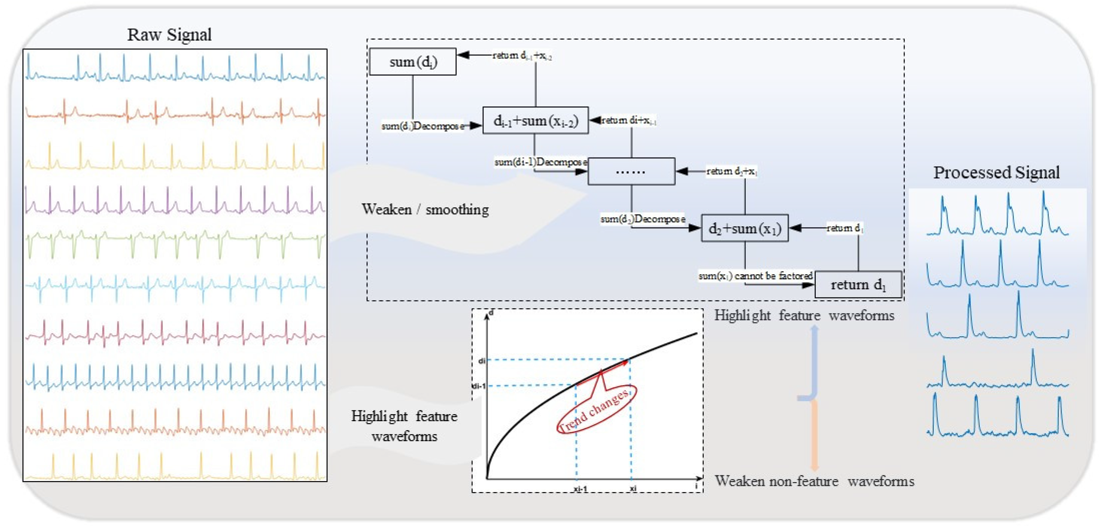
Figure 2. Parameter Setting Process Flowchart.

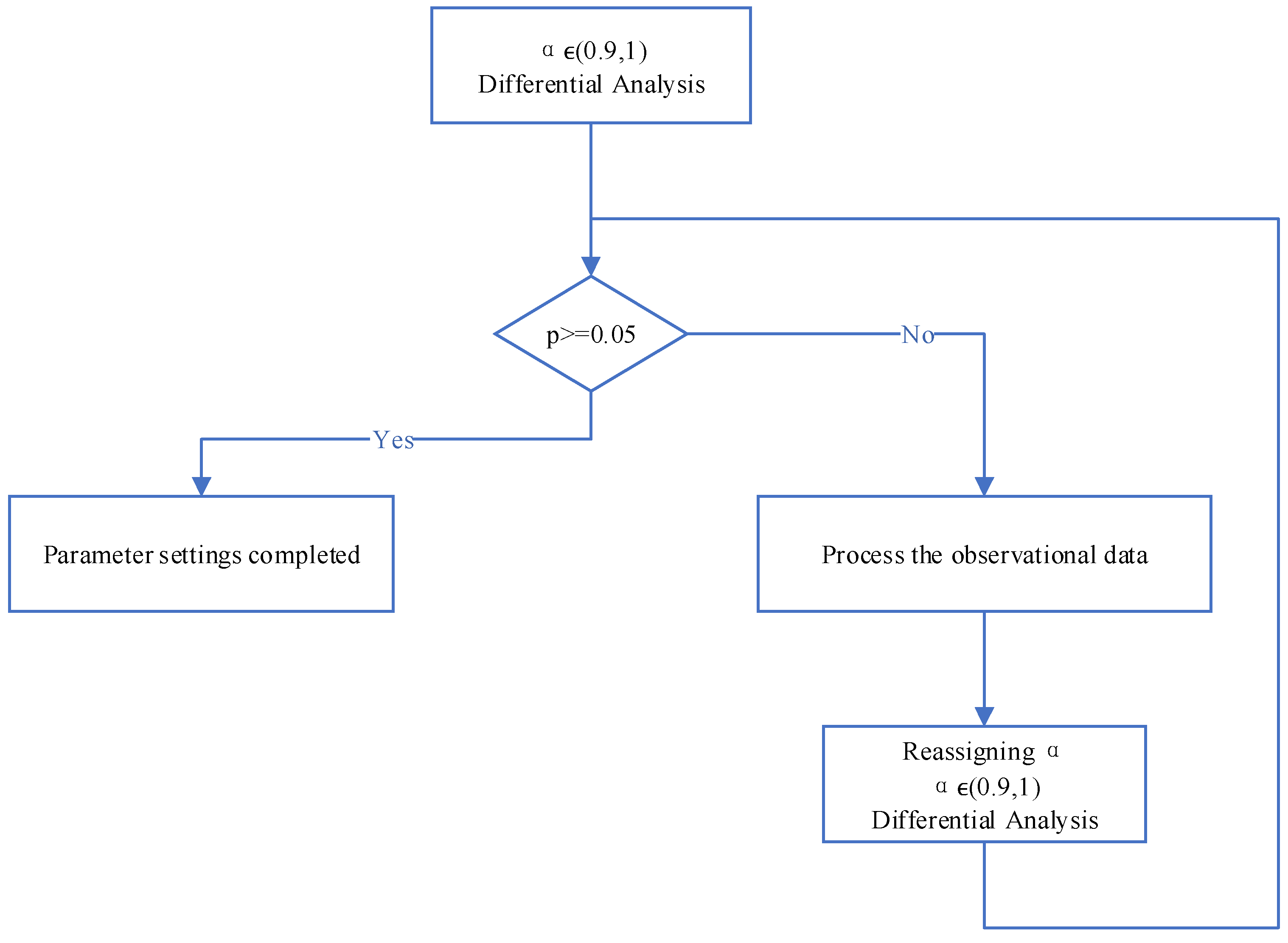
Figure 3. Parameter Setting Steps Based on Differential Analysis.

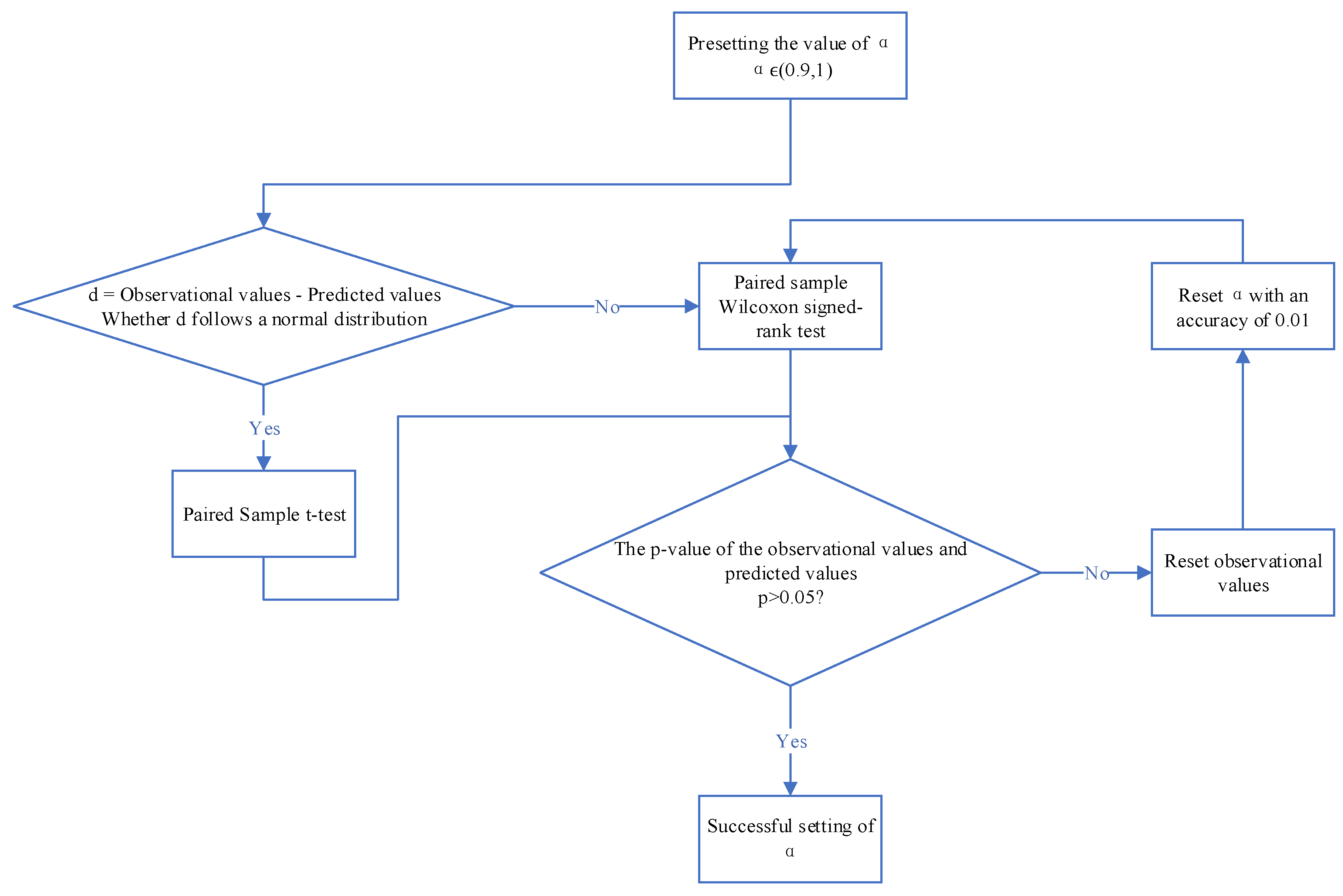
Figure 4. Comparison of Difference Feedback with Absolute Values. The Top Figure: Clinical ECG Data of 500Hz, 10s. The Middle Figure: Output after Formula (2). The Bottom Figure: Output of Formula (2) without Absolute Values.

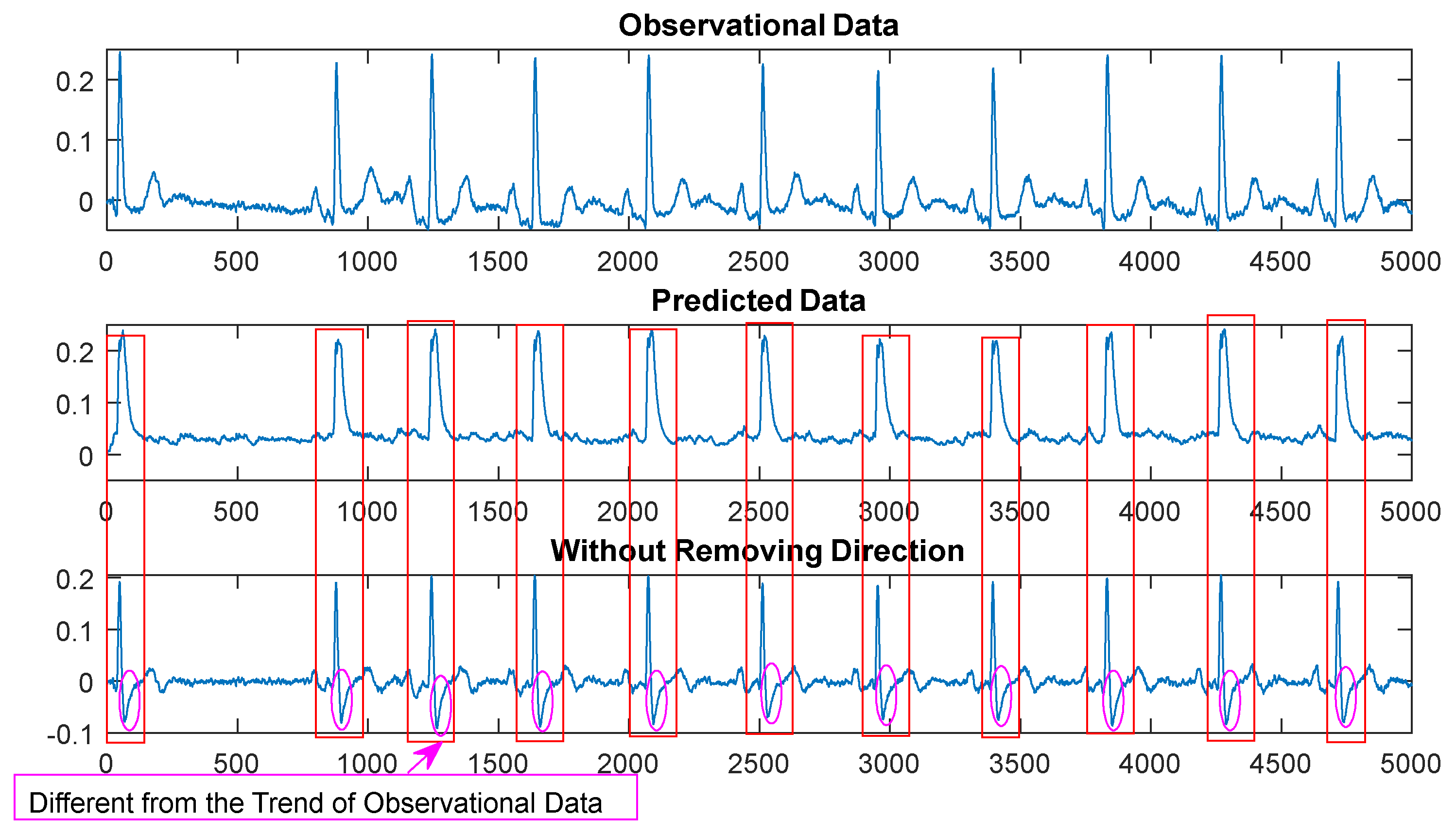
Figure 5. Clinical ECG Data - 10 Typical Conditions. Top Image: Raw Data. Bottom Image: Data after Model Processing.

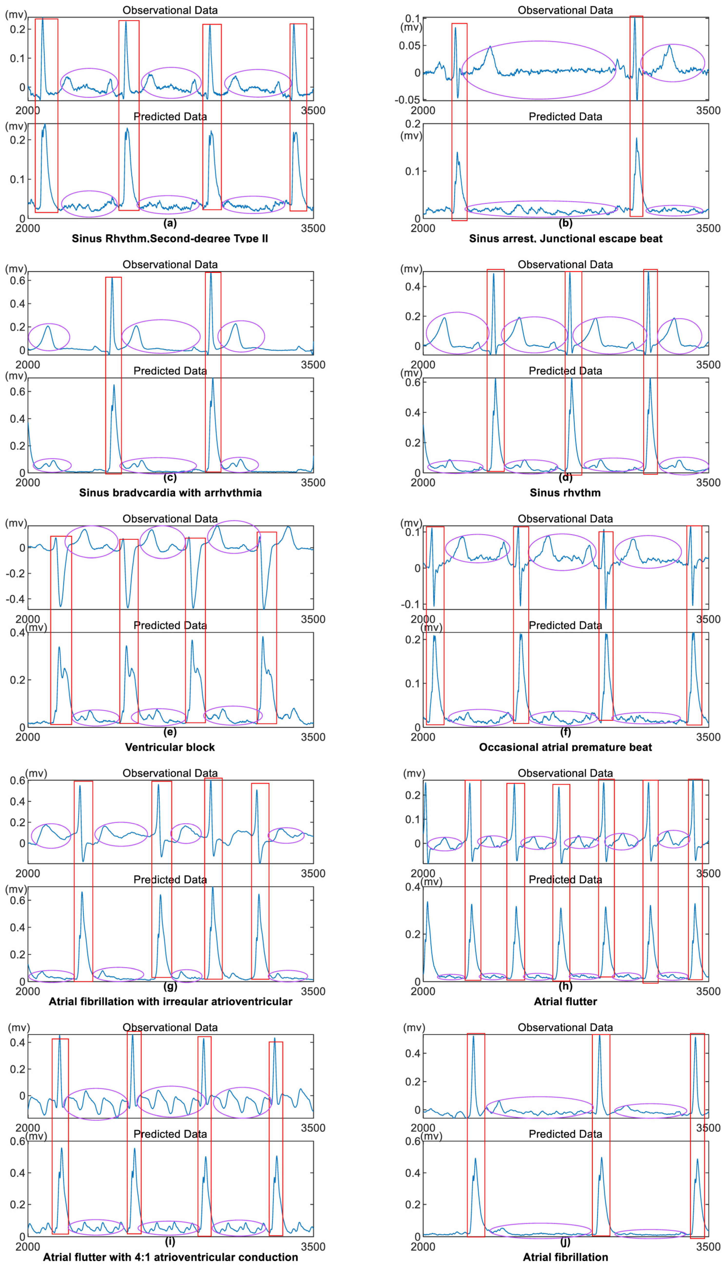
Figure 6. 10 Different ECG Data Samples from MIT-BIH Database Lead II. Top Image: MIT-BIH Data, Bottom Image: Data after Model Processing. (a): From the 90th second. (b): From the 990th second. (c): From the 790th second. (d): From the 900th second. (e): From the 790th second. (f): From the 680th second. (g): From the 480th second. (h): From the 400th second. (i): From the 270th second. (j): From the 200th second.

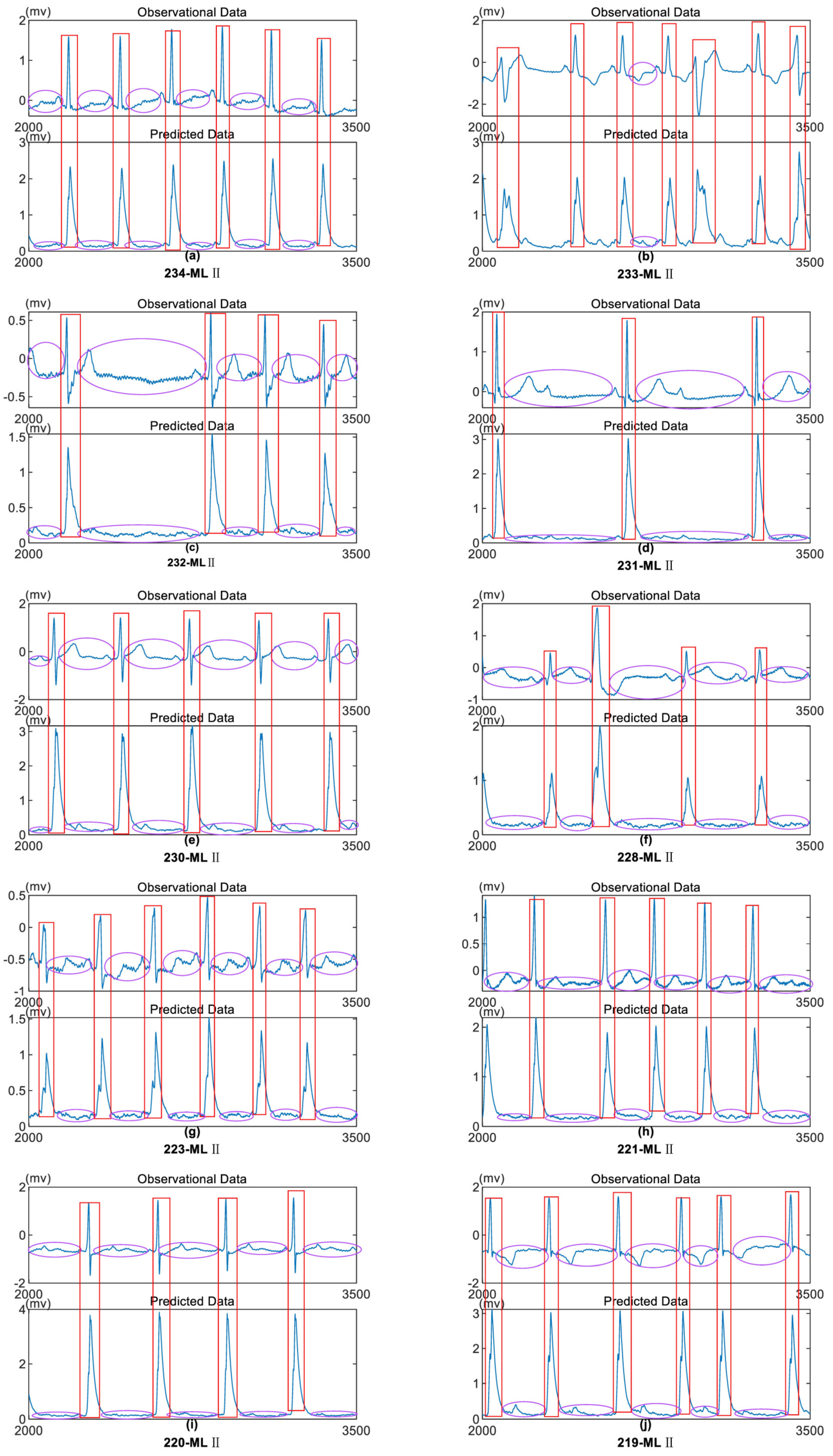
Table 1. Test of Normality for the Residuals of Observational and Predicted Values.

	Kolmogorov-Smirnova			Shapiro-Wilk
	Statistic	df	Sig.	Statistic	df	Sig.
D_value	.163	5000	.000	.810	5000	.000

¹ Lilliefors Significance Correction. ² D_value:

d_{1} - y_{1}

α = 0.94

Table 2. Result of Paired Sample Wilcoxon Test for Two Groups of Data d1 and y1.

d_{1}

: raw data,

y_{1}

: Output data of the algorithm model when

α = 0.94

Table 2. Result of Paired Sample Wilcoxon Test for Two Groups of Data d1 and y1.

d_{1}

: raw data,

y_{1}

: Output data of the algorithm model when

α = 0.94

		N	Mean Rank	Sum of Ranks
$y_{1} - d_{1}$	Negative Ranks	192^a	347.70	66759.00
	Positive Ranks	4791^b	2577.93	12350877.00
	Ties	17^c
	Total	5000
			$y_{1} - d_{1}$
Z			-60.480^d
Asymp. Sig. (2-tailed)			.000

¹ a.

y_{1}

< Real. ² b.

y_{1}

> Real. ³ c.

y_{1}

= Real. ⁴ d. Based on negative ranks.

Table 3. Result of Paired Sample Wilcoxon Test for the Predicted Data and the Reset Observational Data Corresponding to Different Values of

α

Table 3. Result of Paired Sample Wilcoxon Test for the Predicted Data and the Reset Observational Data Corresponding to Different Values of

α

		N	Mean Rank	Sum of Ranks
	Negative Ranks	52^a	48.47	2520.50
Predicted data α=0.94	Positive Ranks	59^b	62.64	3695.50
Reset raw data α=0.94 Predicted data α=0.95 Reset raw data α=0.95 Predicted data α=0.93 Reset raw data α=0.93	Ties Total Negative Ranks Positive Ranks Ties Total Negative Ranks Positive Ranks Ties Total	4889^c 5000 27^d 83^e 4890^f 5000 70^g 41^h 4889ⁱ 5000	26.59 64.90 60.04 49.10	718.00 5387.00 4203.00 2013.00
	Predicted data-Reset raw data, α=0.94	Predicted data-Reset raw data, α=0.95	Predicted data-Reset raw data, α=0.93
Z Asymp. Sig. (2-tailed)	-1.729^j .084	-6.963^j .000	3.222^k .001

* a. Predicted data α=0.94 < Reset raw data α=0.94. * b. Predicted data α=0.94 > Reset raw data α=0.94. * c. Predicted data α=0.94 = Reset raw data α=0.94. * d. Predicted data α=0.95 < Reset raw data α=0.95. * e. Predicted data α=0.95 > Reset raw data α=0.95. * f. Predicted data α=0.95 = Reset raw data α=0.95. * g. Predicted data α=0.93 < Reset raw data α=0.93. * h. Predicted data α=0.93 > Reset raw data α=0.93. * i. Predicted data α=0.93 = Reset raw data α=0.93. * j. Based on negative ranks. * k. Based on positive ranks.

Table 4. Consistency and Variability Analysis Results for 10 Typical Clinical ECG Conditions Result: Output Signals after Model Processing.

	Example data	(a)		(b)		(c)		(d)		(e)
Validation metrics		raw	result	raw	result	raw	result	raw	result	raw	result
Variance		6.32E-04	2.21E-04	1.20E-04	6.23E-05	4.18E-03	3.28E-04	3.63E-03	2.28E-04	1.10E-03	1.26E-04
Correlation coefficient		0.996		0.999		0.995		0.996		0.956
	Example data	(f)		(g)		(h)		(i)		(j)
Validation metrics		raw	result	raw	result	raw	result	raw	result	raw	result
Validation		3.60E-05	2.34E-05	4.21E-03	3.01E-05	6.04E-04	6.89E-07	2.41E-03	1.29E-04	2.58E-03	2.20E-05
Correlation coefficient		0.933		0.984		0.990		0.997		0.990

Table 5. Consistency and Variability Analysis Results for 5 Sets of MIT-BIH Database.

	(a)		(b)		(c)		(d)		(e)
Validation metrics	raw	result	raw	result	raw	result	raw	result	raw	result
Variance	2.68E-02	3.07E-04	8.66E-02	5.64E-02	4.82E-03	9.84E-04	2.60E-02	9.28E-04	6.80E-03	2.15E-03
Correlation coefficient	0.998		0.994		0.998		0.997		0.999

Disclaimer/Publisher’s Note: The statements, opinions and data contained in all publications are solely those of the individual author(s) and contributor(s) and not of MDPI and/or the editor(s). MDPI and/or the editor(s) disclaim responsibility for any injury to people or property resulting from any ideas, methods, instructions or products referred to in the content.

© 2024 by the authors. Licensee MDPI, Basel, Switzerland. This article is an open access article distributed under the terms and conditions of the Creative Commons Attribution (CC BY) license (https://creativecommons.org/licenses/by/4.0/).

Copyright: This open access article is published under a Creative Commons CC BY 4.0 license, which permit the free download, distribution, and reuse, provided that the author and preprint are cited in any reuse.

Downloads

Views

Comments

Subscription

Notify me about updates to this article or when a peer-reviewed version is published.

MDPI Initiatives

Important Links

Choose an area of interest and we will send you notifications of new preprints at your preferred frequency.

Disclaimer

Establishment and Application of Recursive Digital Processing Algorithm with Difference Analysis-Based Parameter Setting and Difference Feedback

Abstract

Keywords:

Subject:

1. Introduction

2. Method

2.1. Mathematical Formulation of the Algorithm

2.2. Meaning and Purpose

2.3. Parameter Settings based on Difference Analysis

2.4. Absolute Value Differential Feedback—— y 2

3. Case Study and Discussion

3.1. Clinical ECG Signal

3.2. MIT-BIH ECG Signal

4. Discussion

5. Conclusion

Supplementary Materials

Author Contributions

Funding

Data Availability Statement

Acknowledgments

Conflicts of Interest

References

MDPI Initiatives

Important Links

Subscribe

2.4. Absolute Value Differential Feedback—— $y_{2}$