An Evolutionary Hybrid Convolutional Deep Learning Network to Classify Paddy Leaf Disease

Preprint

Article

An Evolutionary Hybrid Convolutional Deep Learning Network to Classify Paddy Leaf Disease

Altmetrics

Downloads

Views

Comments

This version is not peer-reviewed

Submitted:

19 June 2024

Posted:

19 June 2024

You are already at the latest version

Alerts

Abstract

Rice has become the second major food among rural people. It is one of the most nutrient and low-cost food available in Asia. Rice is composed of two major subspecies as Japonica and Indica and it belongs to the Poaceae family. The World Bank predicts that rice demand will grow 51% faster than population growth in 2025. It is high time to develop a model which predicts the type of infected paddy leaf and avoids the loss of grains. In this paper, the proposed hybrid CNN model, three CNN networks with different layer properties are trained parallel. The extracted feature from these CNN networks is combined to provide the classification of the type of infected leaf. Fieldwork was carried and about 340 samples are collected from five different types of classes. The proposed hybrid model was tested with both the fieldwork dataset and also with an available dataset on the internet. The experimental results show that the proposed model outperforms the other CNN network and yields an accuracy value of 98%, a precision value of 95%, and a misclassification rate of 4% respectively.

Keywords:

Subject: Engineering - Other

1. Introduction

Over the world, the second major food is rice among the rural people. It is the one of the most nutrient and low-cost food available in Asia. Mostly it is cultivated in the region of Europe, Asia, America, Oceania and Africa. Rice is composed of two major subspecies as Japonica and Indica and it belongs to the Poaceae family. As per the statistics shown by the FAOSTAT, more than 90% of the rice crop are cultivated and consumed by the Asian countries [1]. The remaining 10% will be carried out by the other four countries such as Oceania, Europe, America and Africa. 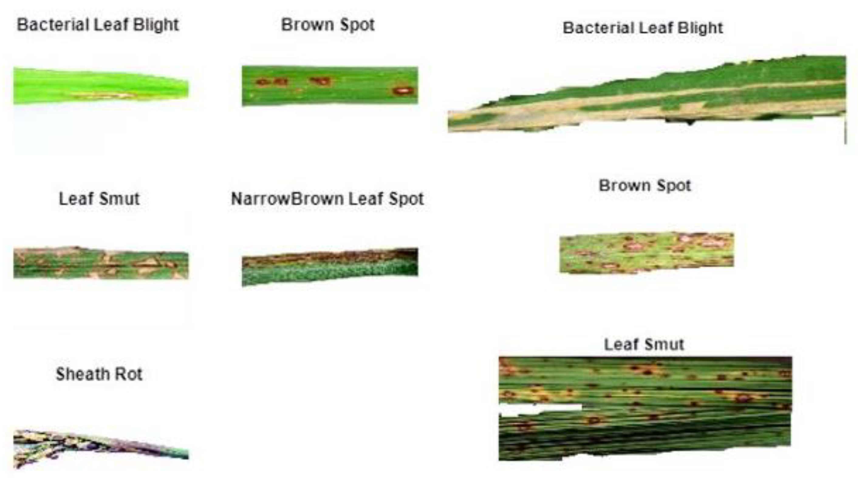The World Bank predicts that rice demand will grow 51% faster than population growth in 2025 [2]. Some of the sample figures from the field work is shown in Figure 1a and from internet is shown in Figure 1b.

False smut, sheath blight, rice blast, leaf scaling, brown spot, bacterial leaf blight, and Bakane are examples of paddy diseases. False Smut is the silvery-white structure that influence panicle development in the late stage. It has a direct effect on paddy yield and is more noticeable during the rainy season when the land has a higher nitrogen concentration and is humid [3]. The second form of paddy disease, sheath blight, infects the straw of the tice and is produced by the Rhizoctonia solani fungus. It happens during the rice harvesting period [4]. The rice explosion is the most common and strongest paddy leaf disease. It happens at almost every stage of rice development, from crop growth to harvest [5,6,7,8]. Node blast, seedling blight, grain spot, leaf blast, and neck blast are all symptoms of this illness. If this type of disease is not treated in advance with proper methodology, the quality and output of grain will be drastically decreased [9,10,11,12]. Leaf scald symptoms include reddish-brown broad bands or golden borders at the leaf edges [13,14,15,16].

In [16] proposed an analysis of insect attack and nutrient deficiency and disease in coconut leaves. Monitoring of coconut leaves after the application of pesticides and fertilizers has been performed using cutting-edge machine learning and image processing methods. SVM and CNN were selected as the best and most suitable classifiers with 93.54% and 93.72% accuracy, respectively. This system has the facility to fully monitor the plant from initial referral to complete recovery.

In [17] propose the correct solution regarding the disease, the identifiable source and the arrangement of the infection. Image processing approaches can automate a number of disease models and pest forecasts. Some types of problems can be identified at an early stage by human vision, while it takes some time to predict. SVM classifier performs better than ANN in detecting yellow rust and septoria with 95% and 70% accuracy, respectively.

In [18] proposed the network was trained to distinguish crop disease using leaf images. The network's several convolutional layers. The image's very basic attributes are extracted in the first few layers, but as we dig deeper, the complexity increases and it can be used to address more intricate issues. In 100 epochs, we were able to achieve 97.50% accuracy for 22 convolution filter sizes, which is superior to other traditional methods.

In [19] suggested a foretelling method using CNN for rice crops to categorize disease predictive. Neural Networks are a collection of complex algorithms modelled after the human brain to recognize different patterns or images. 90.32% accuracy is observed on the test set and 93.58% accuracy on the training set.

In [20] proposed using the NASNet framework for Convolutional Neural Networks (CNNs). Artificial intelligence applications that use deep neural networks have proved effective. One of the main issues, nevertheless, that endangers the availability of sufficient human food is plant diseases. We used different splits including 80%, 60%,50%, 40% and 20%. That is, for example, 80%, 60%, 50%, 40%, and 20% of the total images are reserved for computer training, while the other 40%, 50%, 60%, and 80% are used for validation purposes, respectively.

In [21] Proposed DL as a latest model of ML that uses neural networks that act like the human brain. Early detection and diagnosis of these diseases are critical to the agricultural industry. The system was able to record by the way of classifying and detecting different plant species and plant illnesses, while the trained model had an accuracy rate of 96.5%.

In [22] proposed a model that have already been trained, like VGG19, that are being fine-tuned (transfer learning) to pull out pertinent features from the dataset. pretrained models such as VGG19 that is fine-tuning to extract relevant features from the dataset. Huge amount of data to perform better than other techniques. Potato is a highly versatile crop that contributes about 28.9% of India's total agricultural crop production.

In [23] suggested a method for training deep CNN networks, which need a lot of data and expensive computing power. With the aim of examining the full training and fine-tuning the performance of the CNN, we modified the structure using the bestfit joint model. It is an advanced processing method. ResNet with SGD optimization method achieves the highest test accuracy of 97.28%.

In [24] proposed various image-based CAD systems have been proposed using colour features in agriculture applications. In this work, we have concentrated particularly on the illness of the rice plant (Oryza Sativa). Every year the disease causes huge economic losses to formers. The proposed model can categorize rice diseases with 91.37% classified accuracy for 80%- 20% training-test distribution.

The traditional methods for diagnosing leaf diseases rely on human vision. In these situations, getting expert guidance requires a lot of time and money. The proposed hybrid CNN model mainly focused on identifying various types of diseases present in the leaf of the plant.

For brown spot disease, the symptoms will be dark brown lesions in oval shape occurs in the rice plant leaves. Bacterial leaf blight occurs on leaf tip with elongated lesions. It grows to several inches and becomes as yellow due to the bacterial effects. The last disease in the paddy leaves is Bakane and affects the development phase with abnormal elongation in the seedbed. The major cause of it is the yellow shades leaf with empty panicles, dismissal of the seed at early stage and dehydration of leaves. It looks much higher than normal plants and also widely found in vegetative stage. Therefore, image processing techniques are used to classify paddy leaf diseases. The main contributions of the research work are summarized as follows:

➢: A novel the hybrid CNN model has been proposed to classify the paddy leaf diseases such as bacterial leaf blight, brown spot, sheath rot, narrow brown leaf spot, and leaf smut.
➢: Initially, the input images are gathered from two dataset namely internet dataset and field work dataset.
➢: The collected images are pre-processed using CLAHE filter to remove noise artifacts.
➢: The proposed model is a combination of three CNN network with different layer properties are trained parallel for classification.
➢: The performance of the suggested hybrid CNN is evaluated by using specific performance metrics.

The remaining portions of the analysis are structured as follows: Section II describe the Literature survey in detail. Section III describes the background study of hybrid CNN model. Section IV describes the suggested hybrid CNN model. The result is given in section V and finally section VI describes the conclusion.

2. Materials and Methods

In the paradigms of both supervised and unsupervised, Convolution Neural Network (CNN) model will be the best model for the classification purpose. In the supervised mechanism, the model is learned from the mapping between the desired output and system input. Whereas in the case of unsupervised learning method, the model is trained in such a way to predict the true labels of the given set of input dataset. It is well and good, to understand the architecture and working principle of a CNN before we apply the network to the dataset for the classification purpose. A simple CNN consists of various building blocks referred as CNN layers. It has convolution, normalization, fully connected layers and pooling.

The first stage in the CNN is the pre-processing mechanism; the input image needs to be processed before allowing them to pass through the network. The various methods of data pre-processing are normalization, mean-Subtraction, Local Contrast Normalization, PCA whitening. The normalization method divides the data by its standard deviation. Mean subtraction computes the mean of a dataset and zero-centers it around that mean. In Local Contrast Normalization, a local neighbourhood will be generated first for each pixel, and then it is zero-centered with the mean. In the similar manner, the pixel is also be normalized with respect to the standard deviation. The last pre-processing method is PCA whitening. In this, the data are normalized independently by reducing the correlation between the different dimensions of the data. Initially the data is zero-centered first, and then covariance matrix will be estimated to encode the correlation level between the data dimensions. Using singular value decomposition (SVD) algorithm, the correlation level of the data is decomposed and finally it will be normalized by dividing the data by its corresponding eigen values. To attain stable learning process, mean-subtraction method is widely used, as the PCA whitening results in the amplification of the noise signal along with the data and decays the performance of the network. It is also supportive for the gradient-based learning through mean-subtraction and normalization. It has been proved in the recent research that batch normalization outperforms s the other two normalization methods such as Local response normalization and Local Contrast Normalization. Hence, batch normalization is used in the suggested hybrid CNN network.

The heart of the CNN is the convolution layer; the input data is convolved with the set of the kernels to produce the feature map. Convolution kernels can be also termed as filters in which the dimension of it can be varied by the users. At the start of the training phase of CNN, the weights of each convolution layers are initialized randomly. As the training process progress; the weights are tuned and updated to optimal one for the given pair of the input data with it label. A convolution layer multiplies the input data with the kernels to results in the feature extraction. For example, input data with the dimension of 10x10 convolved with the kernels size of 3x3 results in the feature extraction output with the size of 8x8. These feature data can be down sampled by applying stride in the convolution layer. For the above example, if stride of 2 is applied results in the reduction of the data size from 8x8 to 6x6. In order to maintain the same dimension of the feature data, addition of zeros can be carried and this process is termed as padding. In short input size of 10x10 with kernels size of 3x3, stride value of 2 with same padding result in the feature data size of 8x8.

The third component of the CNN is the pooling layer. It works on the extracted feature output from the convolution layer and combines the activation of the feature data. The two types of pooling layers are mean and max pooling. In the case of mean pooling, the average value of the feature and determined and mapped according to the position of the feature data. The maximum value of the features is evaluated and mapped with respect to the data in the max pooling layer. This pooling operation can be termed as down sampling as it reduces the dimension of the extracted features considerable. The last component of the CNN network is the fully connected layers. It acts like a bridge between the output of pooling layer and number of classes. In most the case, the dimension of the pooling layers will not match with respect to the number of classes, in such a case, fully connected layer will be used. The operation of fully connected layer is matric multiplication followed by vector addition and generally it is placed at the end of the CNN architecture.

2.1. Proposed Hybrid CNN Model

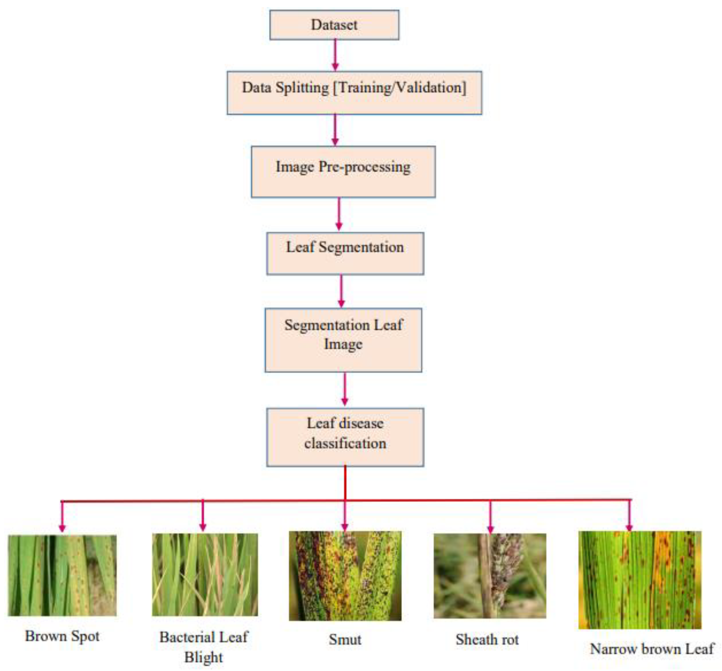
In this section, a novel hybrid CNN model for classifying the blight and spot diseases of the paddy crops as shown in Figure 2. In the pre-processing stage, CLAHE is used to increase the worth of image.

2.1.1. Dataset Description

Internet dataset;

Data set 1 (Internet dataset) consists of 120 images with three different classes of infection: BLB, BS, and LS. Of these, 105 images are used for the training process and the remaining 15 images are used for the validation process.

Fieldwork dataset;

Dataset 2 (Fieldwork dataset) consists of five different classes namely BLB, BS, LS, NBLS, and SR. In the dataset 2, there are 345 images. To train the network, 175 images were used and the remaining 65 images are used for the validation process.

2.1.2. Dataset Pre-Processing

The relative region of an image with adaptive histogram equalization (AHE) tends to have too much noise amplitude. Contrast-Limited Adaptive Histogram Equalization (CLAHE), a variation of Dynamic Histogram, tries to prevent over-amplification by restricting contrast. To produce the enhanced effect, CLAHE was applied. CLAHE was applied when the summary was a degree of decompression to the second-to-last in order to prevent a blocking effect. The high-frequency component at this time was improved by the low-frequency element. Finally, following the image restoration, CLAHE was employed.

The image contrast can be altered by the distribution is redistributed of the image histogram. Histogram equalization, which can increase the dynamic range of the pixel grey value, is essentially a mapping change of the original image's grey level. Thus, the contrast of the image can be improved.

Suppose the greyscale of an image’s size range is [0, m−1], with a grey condition of m. Let (s) be the grey-condition of probability density function (PDF). Then, the probability of the kth grey condition is,

(1)

Where, t=0, 1, 2, …, n−1 and stand for the tth greyscale. Then, the K(st) is a cumulative distribution function (CDF) can be revealed as:

(2)

Where, 0 ≤ f ≤ 1

The stages of CLAHE are:

(1): Divide the input image into regions that are unceasing and don't overlap. The standard setting for the region size is 5×5.
(2): Obtain the histogram for each section, then trim the histogram using the threshold. By clipping the histogram with a predetermined threshold prior to calculating the CDF, the CLAHE algorithm achieves the purpose of restricting the magnification. It controls the slope of the transform function
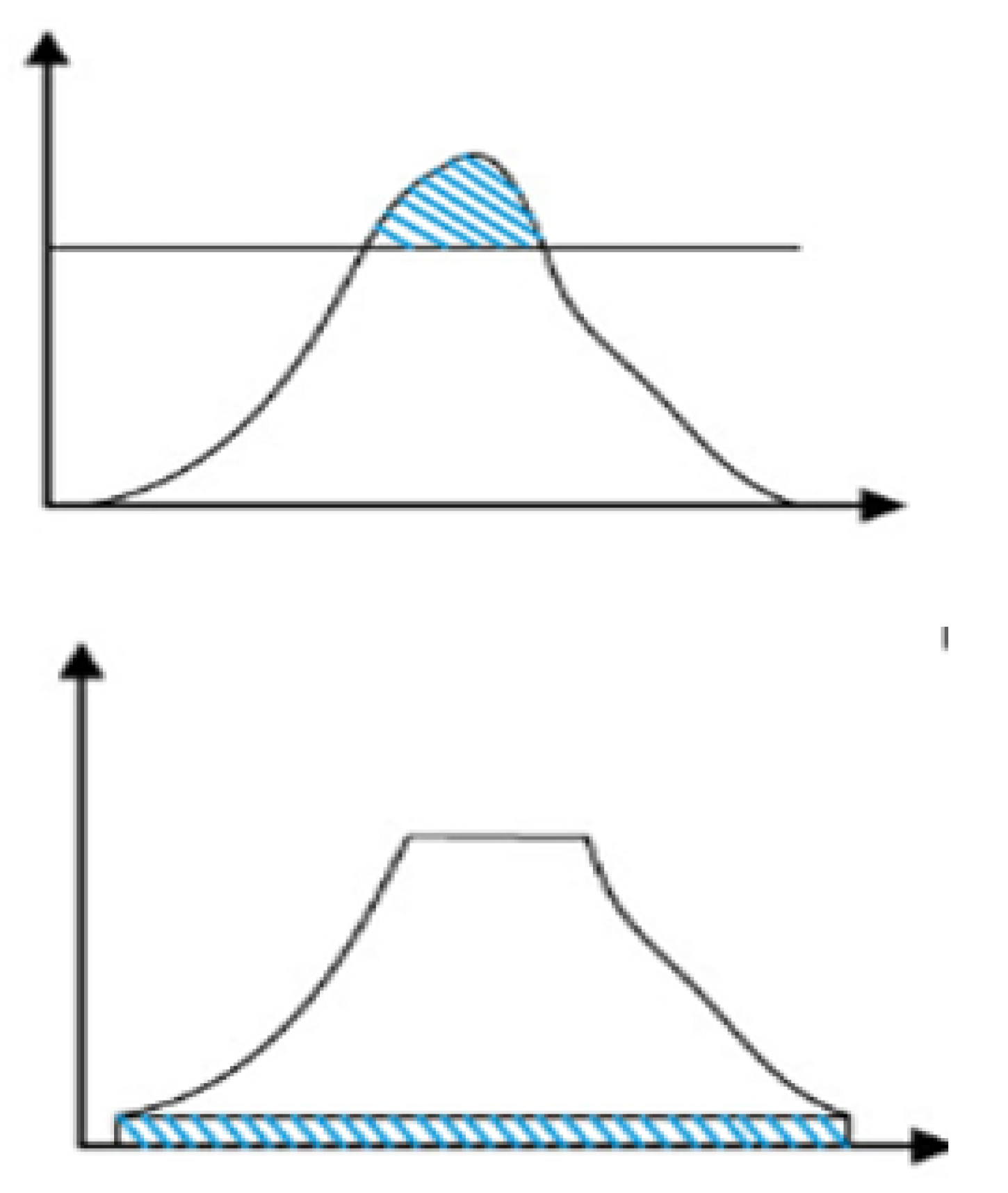
(3): Reassign the pixel values, and then uniformly distribute the clipped pixel values below the histogram. The histogram distribution before and after clipping are shown in figures a and b, respectively.

(4): On each region, carry out a local histogram equalization.
(5): When reconstructing pixel values, use a linear interpolation. Assume that the sample point q' r grey value is r, and that the new grey value obtained using linear interpolation is r'. The surrounding areas' sample points are q1, q2, q3, and q4, and the corresponding r's grey level mappings are fq1 (r), fq2 (r), fq3 (r), and fq4 (r). The new grey value for pixels in the corners corresponds to the region's r's grey-level mapping.

(3)

The interpolation of the grey-condition mapping of r of the two samples of the surrounding areas creates a new grey value for the pixels at the boundaries. For example:

(4)

The interpolation of the r-valued in the grey-condition mapping of the four models from the surrounding areas creates the new grey value for the pixels of the image's centre. For example

(5)

Where, α and β are the normalized distances from the location r1.

Figure 3. Histogram distribution: (a) Initial clipping (b) Final clipping.

2.2. Hybrid CNN

A deep learning model called CNN is used to interpret data with a grid structure, such pictures. CNNs are designed to automatically and adaptively capture spatial hierarchies of information from low-level to high-level patterns inspired by the visual cortex of animals. Convolutional, pooling, and fully-connected layers are three different types of layers (or "building blocks") that often make up a CNN. Convolution and pooling, the first two layers, extract features, and the fully connected third layer, which produces the final output, such as classification, from the extracted features. CNN is a convolution layer, a particular type linear process, made up of a number of mathematical operations. CNN is made up of three layers: convolutional, pooling, and fully connected. The nonlinear ReLU activation function used in the convolutional layer is followed by dropout regularization. Convolution layers are composed of a variety of convolution kernels for extracting input data. The convolution kernels of the convolution layer use convolution operations to apply to the input data in order to extract features. The fully connected layer's FC layer receives flattened input data from the layers above before using it. It is at this moment that the classification process begins. The prediction is processed by the dense layer with softmax using the probability of the score.

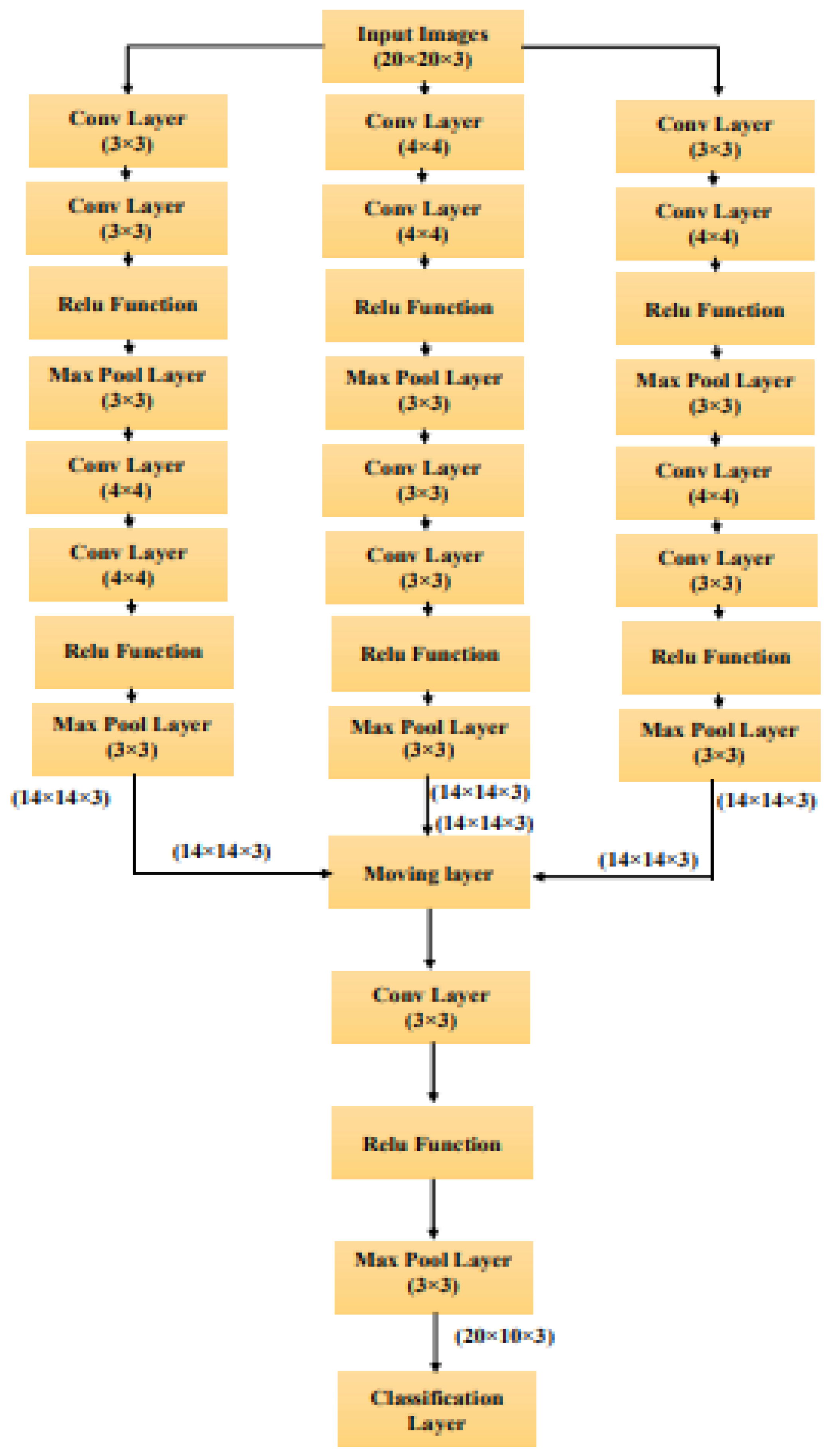
The proposed hybrid CNN consists of three CNN networks followed by a mixed layer of CNN layers. The CNN network accepts an image of pixel size 28 x 28 x 3 and finally outputs feature max pooling layers and ReLU activation functions. In the first CNN network, the input image is processed by two convolutional layers with 16 filters. The first set of each convolutional layer has a kernel size of 3, the second set of convolutional layers has a kernel size of 4, and the extracted features are 14x14x3 using two maximum levels of pooling.

The diagrammatic representation of the proposed hybrid CNN network is shown in the Figure 4. Architecture of Second CNN network is similar to the first CNN network with little modification. It also consists of two set of convolution layer with max pooling layer and ReLU activation function. The kernel size of convolution layer will be 4 in the first set of convolution layer and 3 kernel size in the second set of convolution layer. In the third CNN network, the input image is processed with two convolution layers with 16 filters and has 3 and 4 kernel size during the convolution process. Later these features are given to ReLU activation function to attain the linear output and down sampled with the factor of 2 using max pooling layer and results in the image size of 21x21x3. This process is repeated again to yield the processed image size of 14x14x3.In the mixing layer, the mean output of the three CNN network is accepted and converted into image size of 10x10x3 using convolution layer with 16 filters and kernel size of 3 followed by down sampling with the factor of 2.

Finally, the classification layer is applied to classify the images according to the type of diseases. For field work image dataset, the classification falls into five categories such as BLB, BS, LS, NBLS and SR. In the case of internet dataset, classification will be done based on three classes namely BLB, BS and LS.

Figure 4. Diagrammatic representation of proposed Hybrid CNN Network.

3. Results

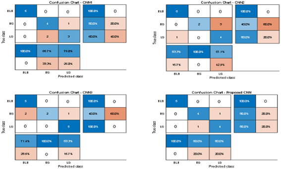
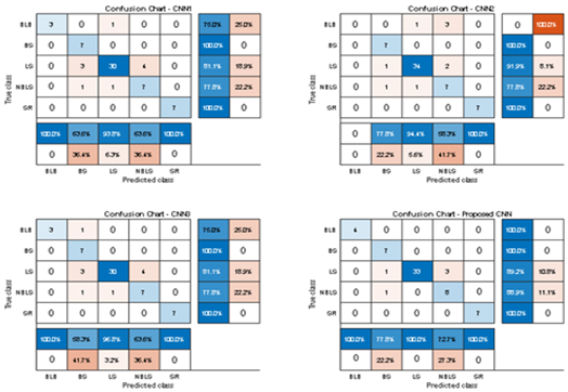
For the simulation purpose, two different datasets are used. Dataset 1 was downloaded from the internet. Dataset2 images are collected through field work. Both datasets are trained to four different models and its confusion chart are shown in the Table 1 and Table 2.

System with Intel core i3 processor with 1.70 Ghz speed, 64-bit processor with 4 GB RAM was used for the simulation purpose. The MATLAB version 2018b was installed in the system and classification of infected paddy leas was carried out. The input image has different pixel size. To maintain the uniformity and reduce the processing time, all the image in the dataset is initially resized into the pixel size of 22x22x3. During the training phase of the CNN network, augmented image dataset is used with the Epoch value of 120, Validation Frequency of 30 and ‘sgdm’ solver.

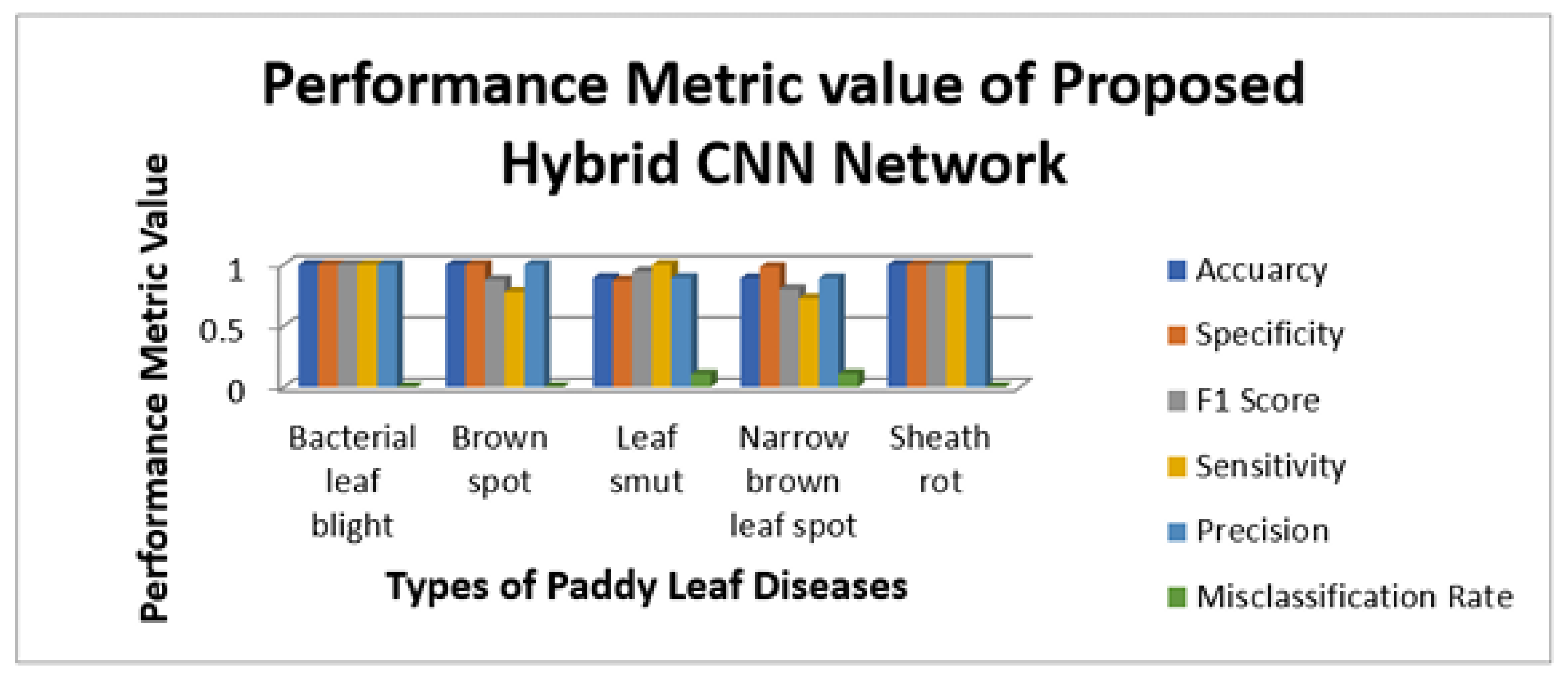
Table 1 which illustrates the efficiency confusion matrix of internet dataset. The actual class of the system is listed as row wise and predicted class as column wise. Basically, it has four terms namely TP means True Positive, TN means True Negative, FP means False Positive and FN means False Negative. Using this confusion matrix, it can analyse the performance of the model through few matric values such as Specificity, Accuracy, F1 Score, Sensitivity, Precision and Misclassification rate. It shows that, the proposed hybrid CNN results in the considerable increase in the accuracy percentage.

This section may be divided by subheadings. It should provide a concise and precise description of the experimental results, their interpretation, as well as the experimental conclusions that can be drawn.

Sensitivity and specificity metrics for two classes can be easily defined and computed in the much simple way. Whereas in the case of the multi-class classification problem, determining these values are bit complicated and cumbersome process. Basically, specificity is defined as the ratio of the true negative class to the total number of normal paddy leaf. The ratio of the true positive to the total number of the disease class is referred as the sensitivity.

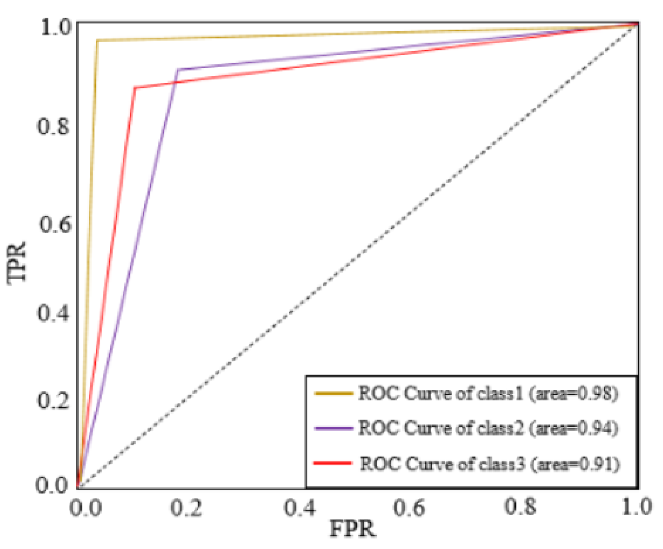
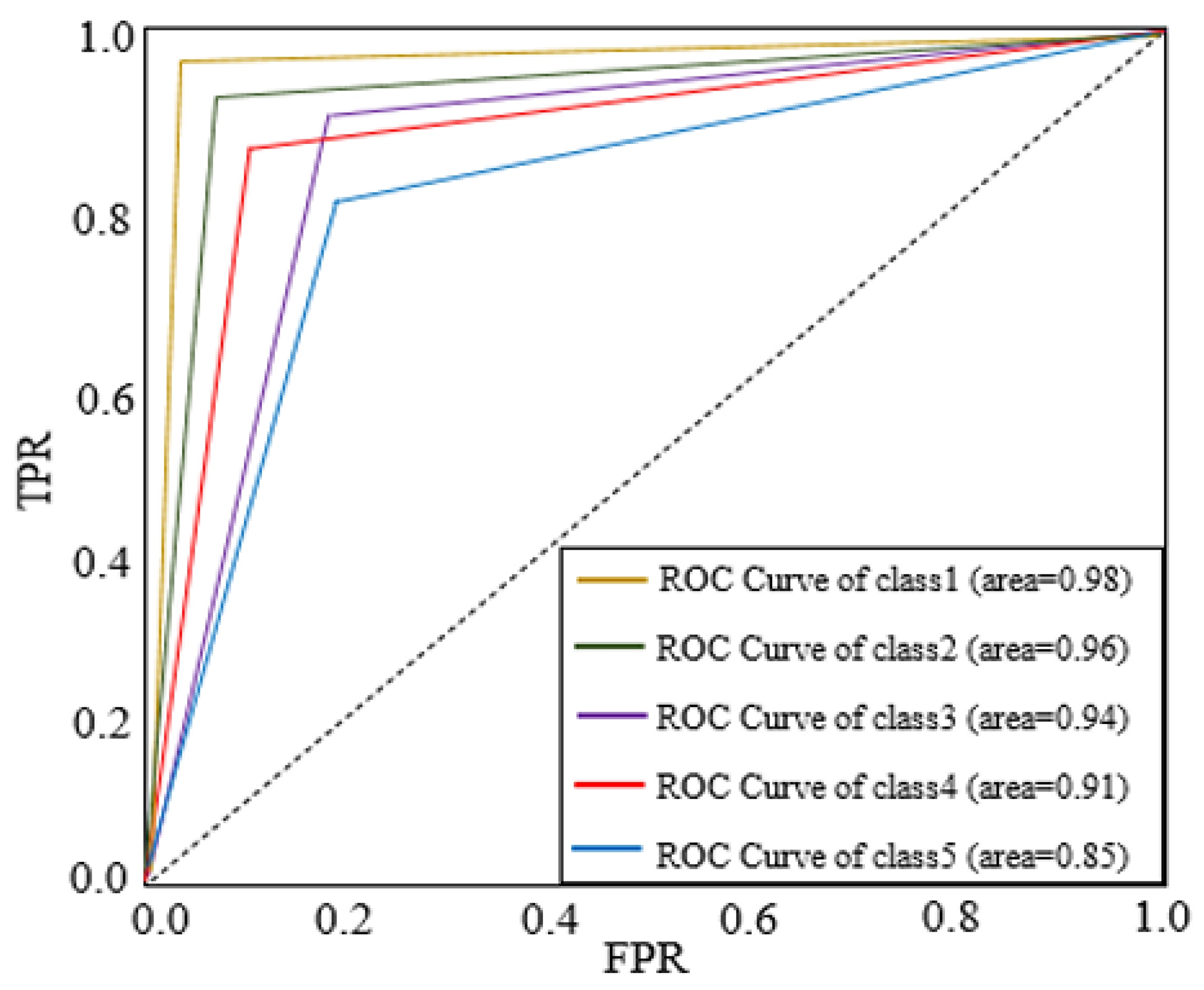
The ROC curve for the features is depicted in Figure 5 using images from internet dataset. BLB, BS, and LS parameters can be used to measure the dataset, the proposed Hybrid CNN method technique achieves greater accuracy.

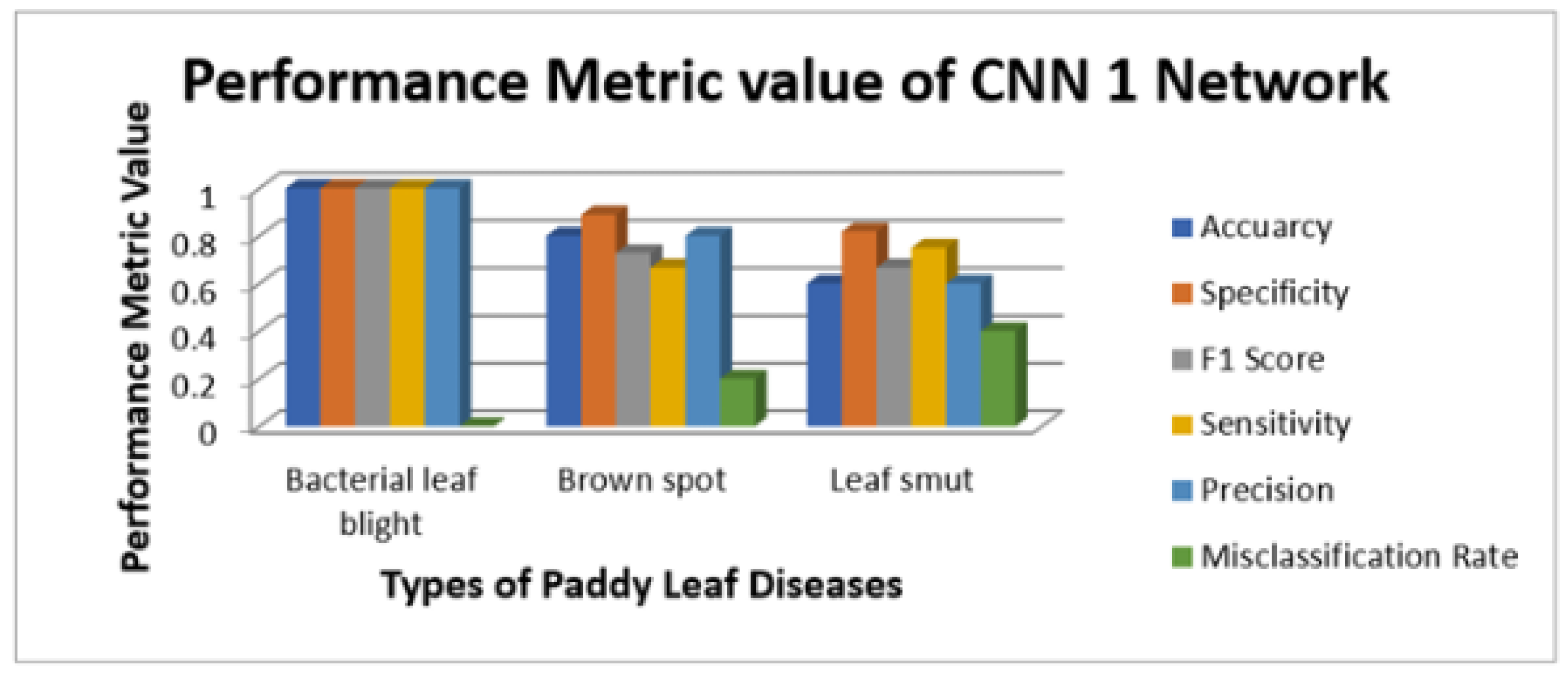
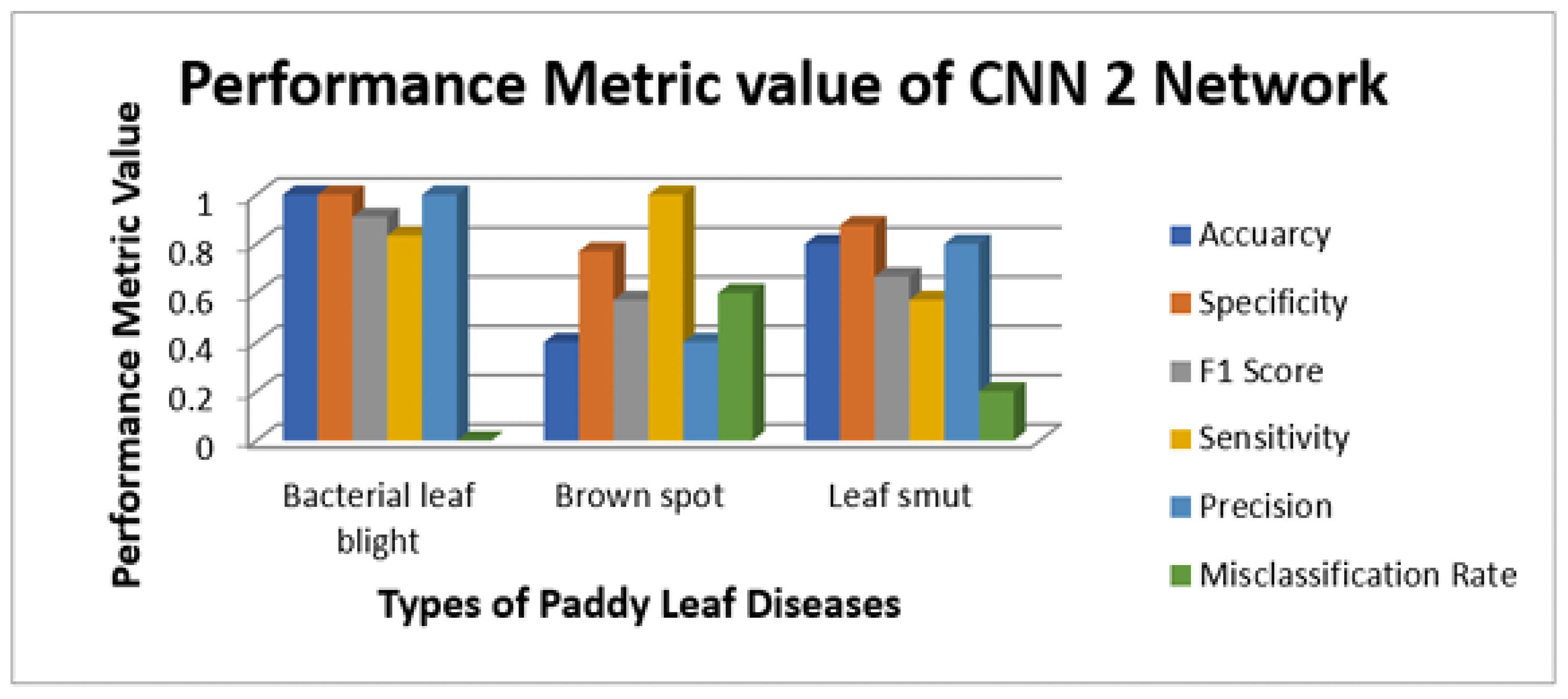
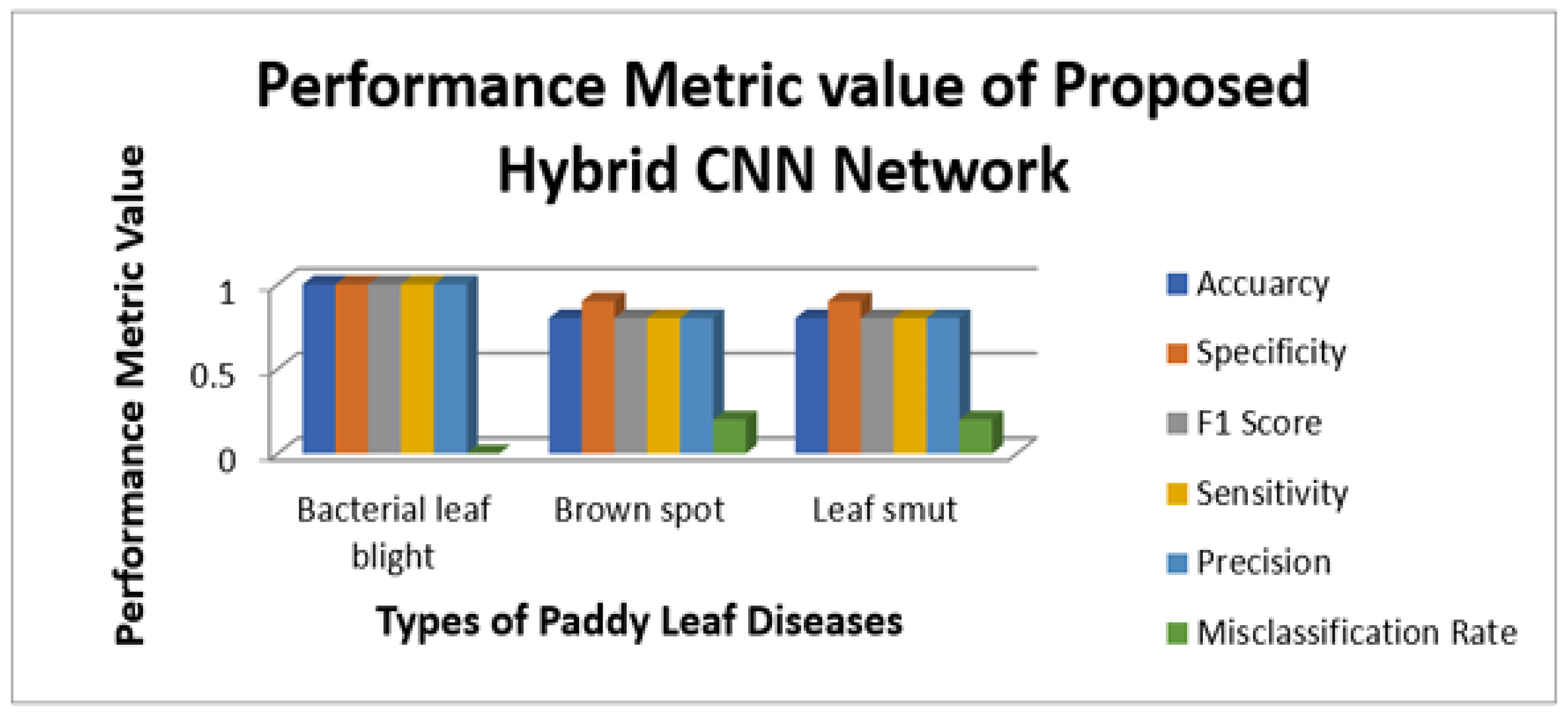
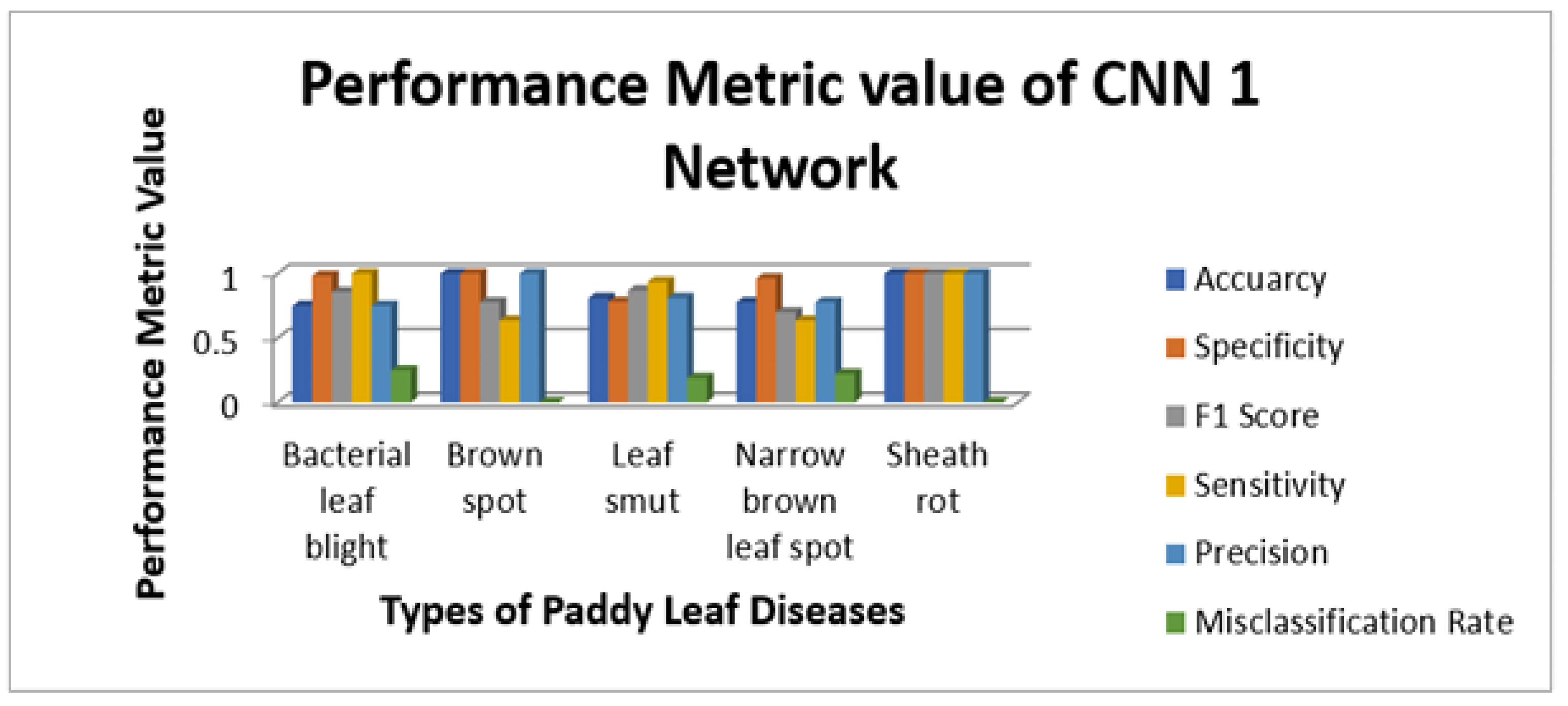
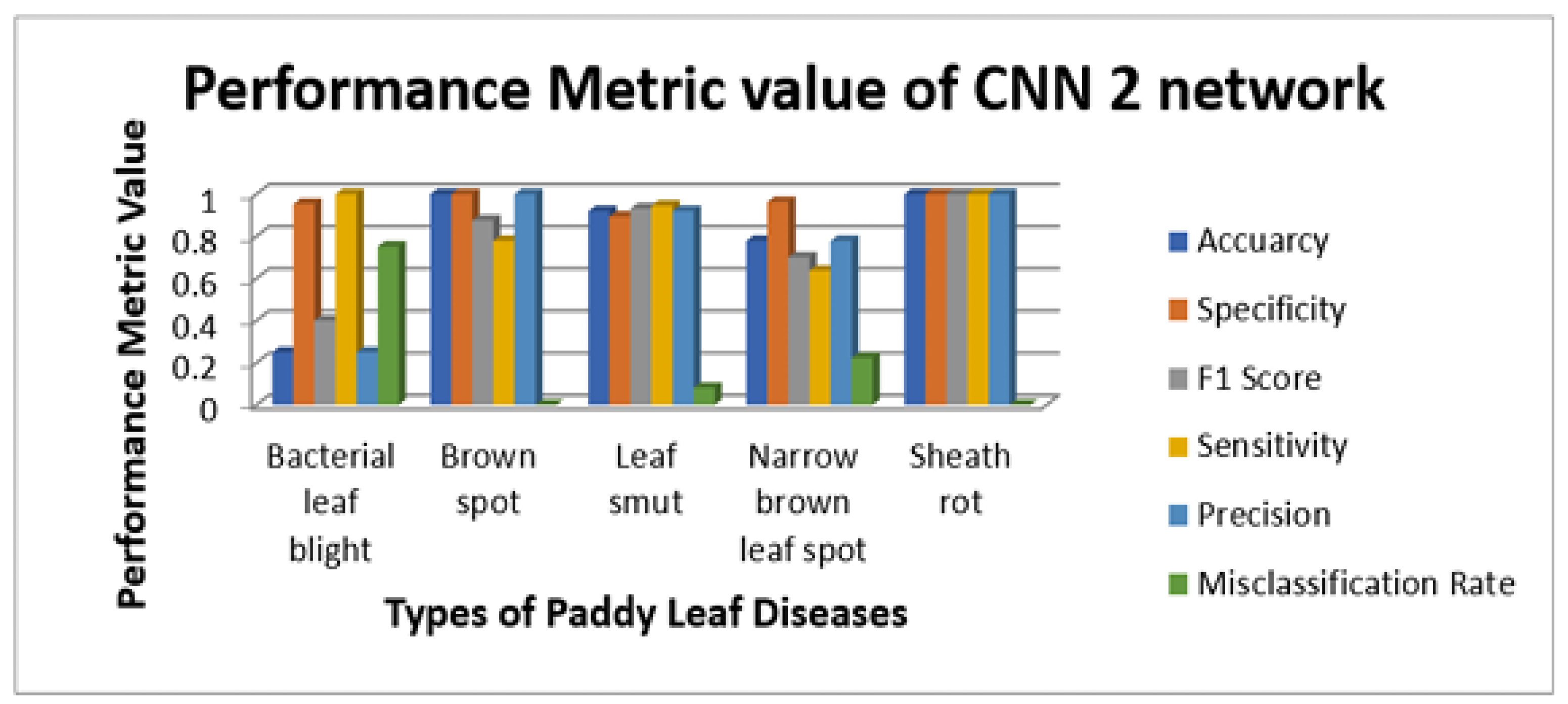
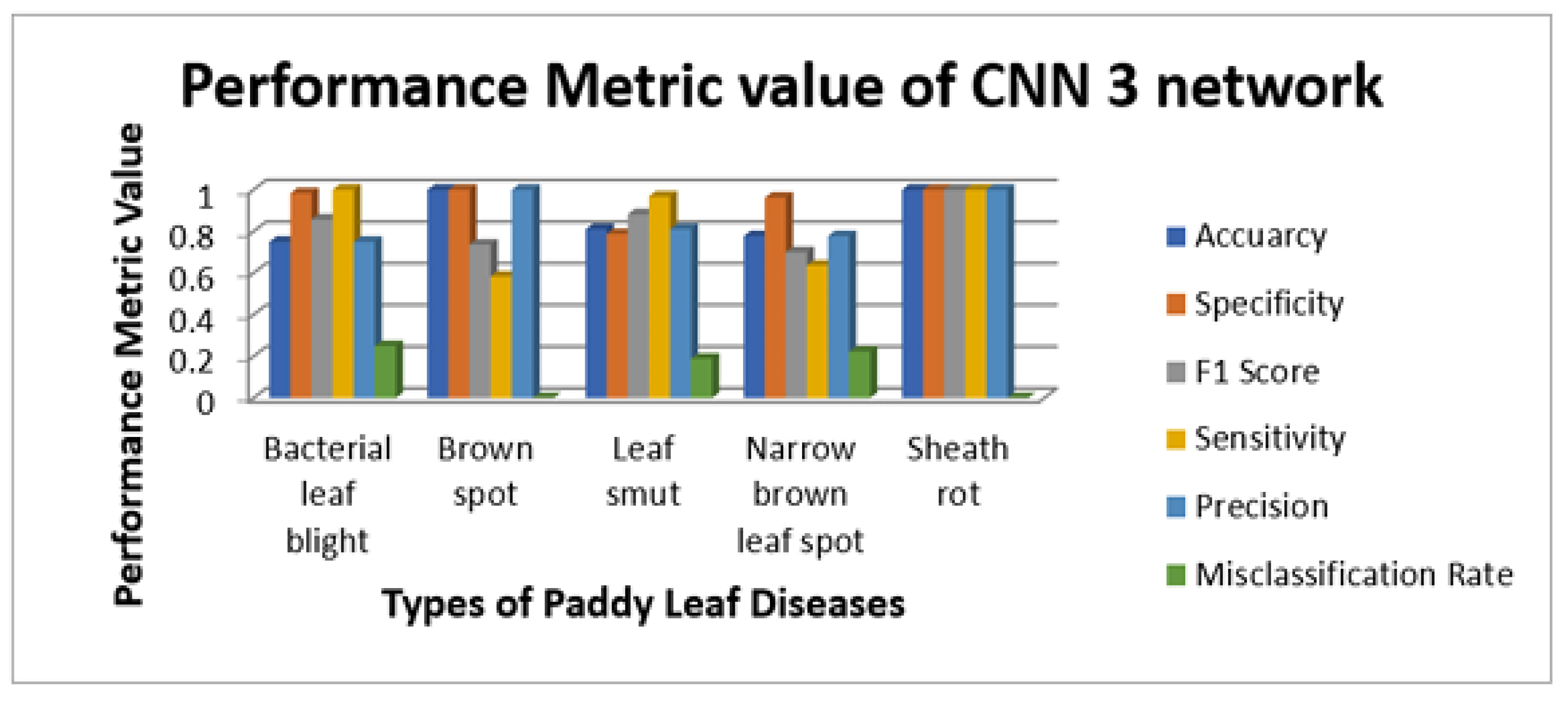
Figure 5, Figure 6, Figure 7, Figure 8 and Figure 9 illustrate the sensitivity and specificity value for the three CNN and proposed Hybrid CNN model for the Internet dataset as bar chart. Internet dataset has three different leaf diseases namely BLB, BS, and LS. To attain the overall specificity value, we can have determined the specificity value individually for each class separately and then average of these values needs to be determined. The CNN1 network predicts the 12 class correctly out of 15 results in the accuracy percentage of 90%, In the same way CNN2 and CNN3 network predicts 11 and 12 classes correctly leads to the accuracy rate of 83% and 85% respectively. The proposed Hybrid CNN outperforms the CNN models and predicts the 13 classes correctly and results in the overall accuracy percentage of 97%.

Table 2 which illustrates the efficiency of the confusion matrix by (Fieldwork dataset). The actual class of the system is listed as row wise and predicted class as column wise. Basically, it has four terms namely TP, TN, FP and FN. In terms of classification of paddy leaf, true positive means that image is infected paddy leaf and trained model predict it as correctly as infected paddy leafThe ROC curve for the features is depicted in Figure 10 using images from fieldwork dataset. BLB, BS, LS, NBLS, and SR parameters can be used to measure the dataset, the proposed CNN method technique achieves greater accuracy.

Figure 11, Figure 12, Figure 13 and Figure 14 illustrate the sensitivity and specificity value for the three CNN and proposed Hybrid CNN model for the field work dataset as bar chart. Field work dataset has five different leaf diseases namely BLB, BS, LS, NBLS, and SR. To attain the overall specificity value, we can have determined the specificity value individually for each class separately and then average of these values needs to be determined. Field work dataset which consists of 64 images, the CNN1, CNN2, CNN3 and proposed Hybrid CNN model will predict the 54, 45, 54 and 59 images in the proper sense and result in the accuracy rate of the 84.37%, 70.31%, 84.37% and 92.18% respectively.

5.1. Comparative Analysis

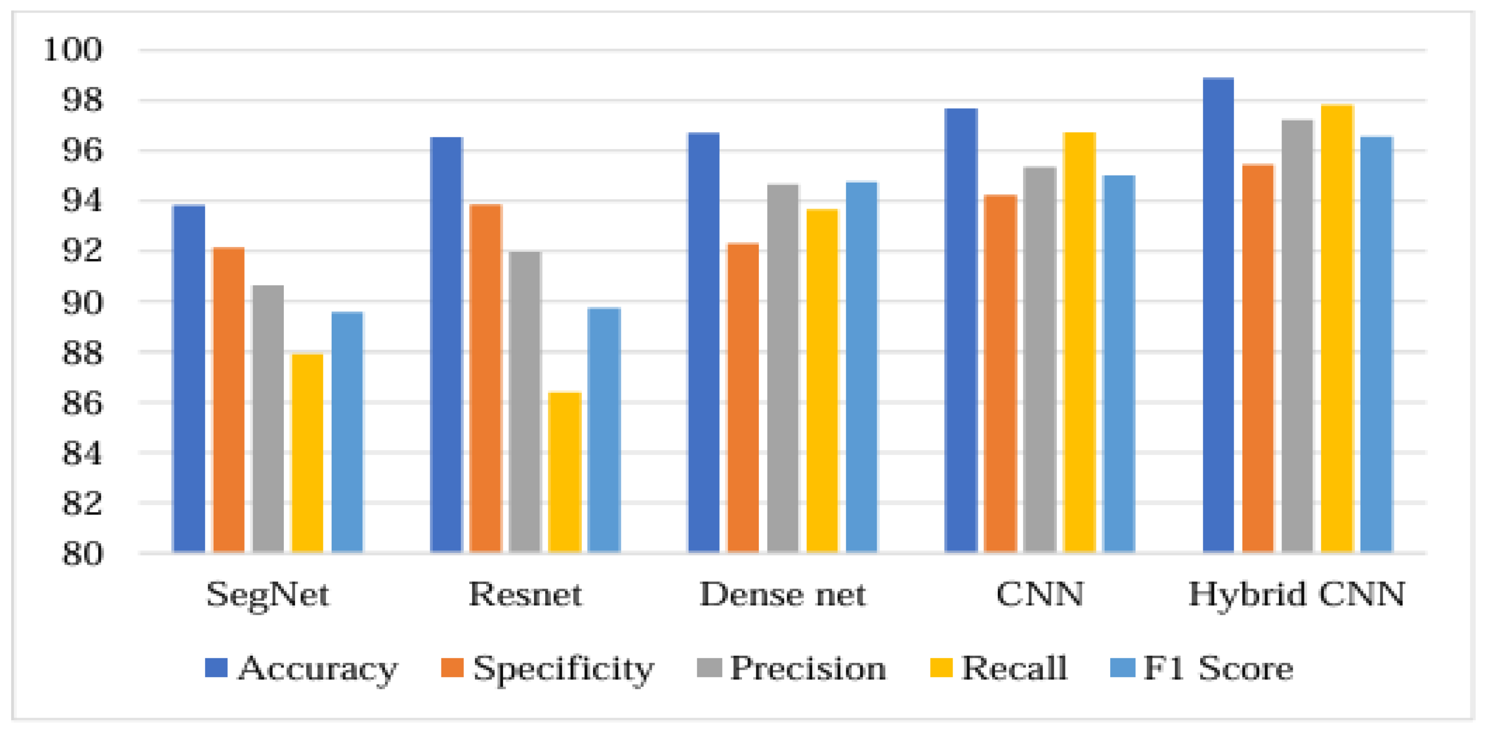
A comparative evaluation between conventional neural networks and the proposed model is also conducted in this division. This technique is more productive than existing methods due to performance comparisons with existing methods. F1 score, precision, specificity, recall, and precision are all used to assess performance. In this comparative analysis, to compare existing deep learning algorithms with our proposed model.

Table 3 shows the final findings in terms of the overall accuracy rate. Table 3 shows that conventional networks such as segnet, Resnet, Dense net, CNN, are lower accuracy than the Hybrid CNN. Hybrid CNN maintains excellent accuracy range of 98.89%.

Figure 15 shows that the accuracy obtained by Seg net, Resnet, Dense net, CNN and Hybrid CNN is 93.82%, 96.54%, 96.70%, 97.66%, and 98.89% respectively. The specificity obtained by Seg net, Resnet, Dense net, CNN and Hybrid CNN is 92.15%, 93.86%, 92.32%.,94.32%, and 95.45%. Precision is obtained by Seg net, Resnet, Dense net, CNN and Hybrid CNN is 90.64%, 91.97%, 94.65%, 95.34 and 97.23%. Recall is obtained by Seg net, Resnet, Dense net, CNN and Hybrid CNN is 87.92%, 86.39%, 93.67%, 96.72% and 97.80%. F1 score is obtained by Seg net, Resnet, Dense net, CNN and Hybrid CNN is 89.58%, 89.75%, 94.76%, 95.01%, and 96.56%. The accuracy rate achieved by the Hybrid CNN is higher efficient than the existing models. Thus, it is clearly shown as the Hybrid CNN model performs better than existing techniques.

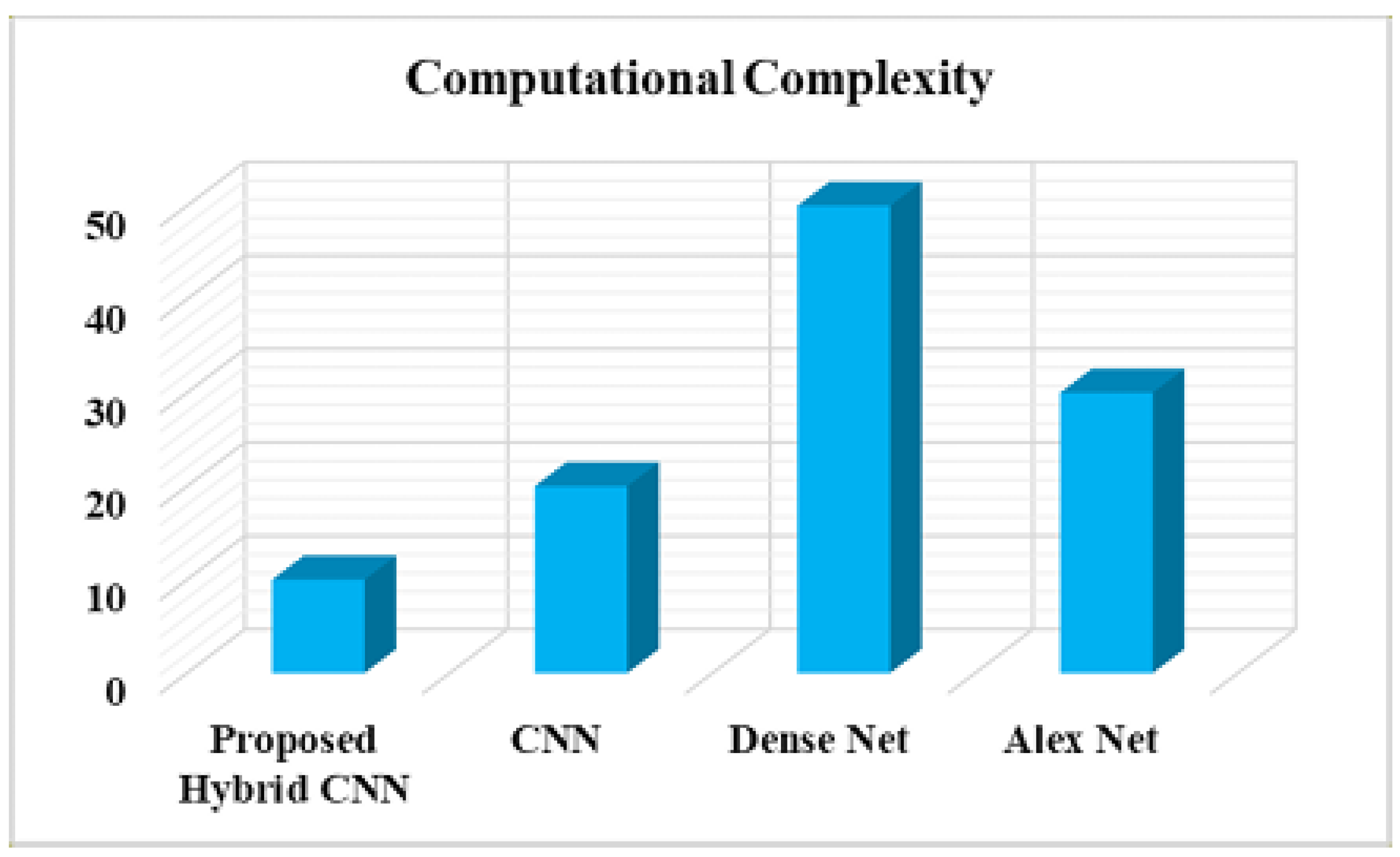
In Figure 16 shows that the Comparison of normalized Computational complexity with respect to hybrid CNN model. The Deep learning networks such as CNN, Dense Net and Alex Net are higher computational complexity than the Hybrid CNN method.

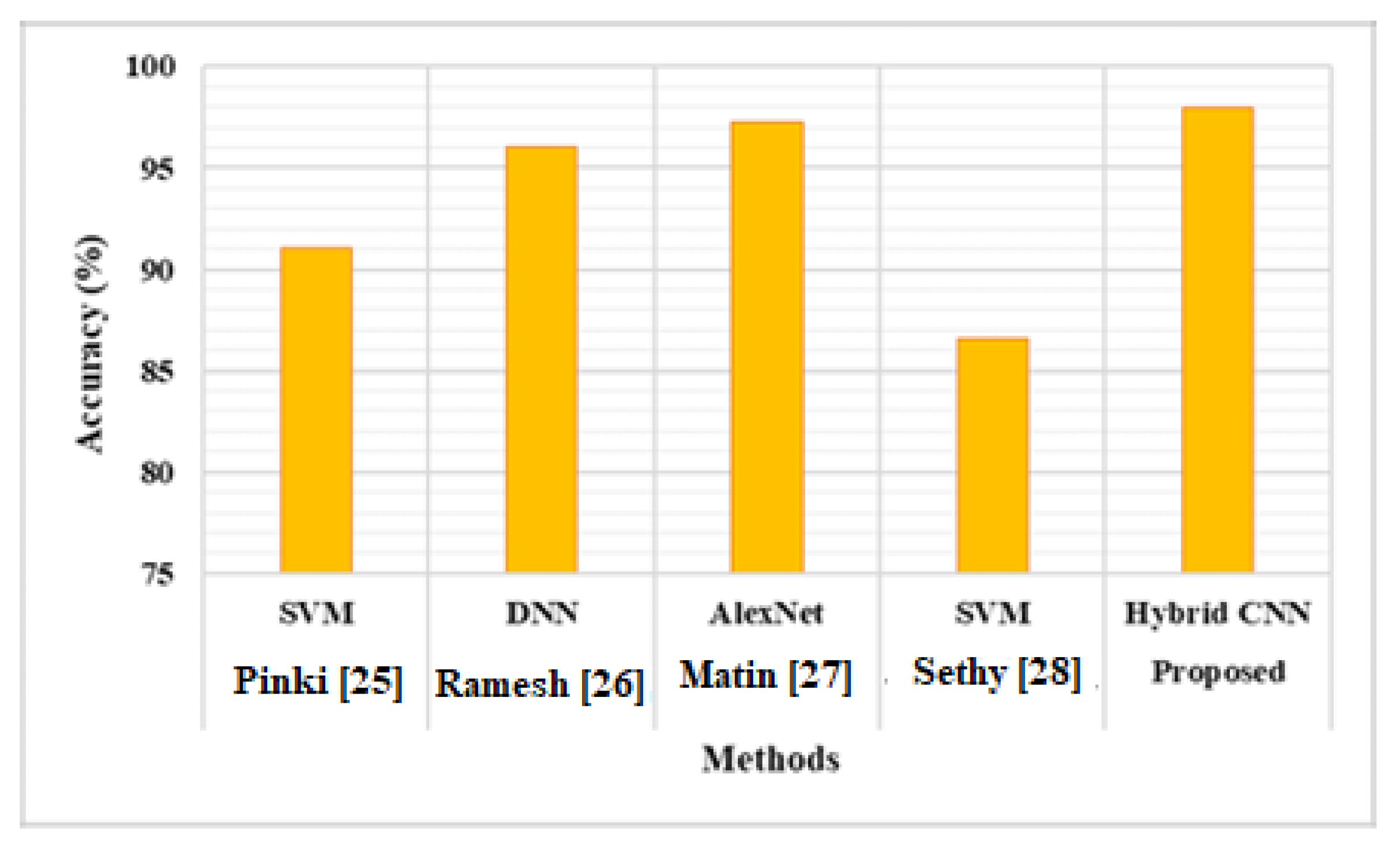
According to Table 3, the suggested Hybrid CNN model improves the overall accuracy of 6.94%, 1.95%, 0.72% and 11.42% better than SVM, DNN, Alexnet respectively.

Figure 17 shows that the proposed hybrid CNN model outperforms the current models in terms of accuracy. In the future, the suggested method's accuracy will be improved in order to correctly segment the diseases and advance the suggested model's accuracy.

5.2. Ablation Study

An ablation study was made to assess the extracted feature from these CNN networks is combined to provide the classification of the type of infected leaf. In this experiment, to comparison CNN1, CNN2, CNN3, and Proposed Hybrid CNN, with the parameters of BLB, BS, LS, NBLS, and SR was illustrated in Table 5. According to our findings, parameters using ablation models was typically less accurate than proposed Hybrid CNN using with CNN2, which proves that the proposed Hybrid CNN using with CNN1, CNN2, and CNN3.

Initially, we have evaluated the effectiveness of the proposed Hybrid CNN and the ablation study is performed with CNN1, CNN2, and CNN3 and without CNN2 method in terms of different parameters. There is a possibility that the model without CNN2 had lowest accuracy in classification. The model for classification the infected leaf uses high level features. The Hybrid CNN model with CNN1, CNN2, and CNN3 had the accuracy in classifying different parameters.

6. CONCLUSION

In this paper, the proposed hybrid CNN model, three CNN networks with different layer properties are trained parallel. The extracted feature from these CNN networks is combined to provide the classification of the type of infected leaf. The experimental results show that the accuracy value of 98% was achieved by the hybrid model, whereas the other three CNN model yields a maximum of 90% accuracy. The proposed CNN model achieved maximum F1 scores of 87% and 91% for the internet and field work dataset. For the fieldwork dataset, the misclassification rate is 20%, 28%, and 20% for the CNN model, a least value of 13% was achieved by the proposed CNN model. In the case of the fieldwork dataset, the rate was further decreased to only 4%. In future work, plan to improve the accuracy using various advanced deep learning techniques or optimized algorithm for accurate and different type of leaf diseases classification and to increase both Training and testing datasets based on diversity and size.

Author Contributions

“The authors confirm contribution to the paper as follows: Conceptualization and methodology: R Sherline Jesie and M S Godwin Premi; software, validation, formal analysis and investigation: R Sherline Jesie and M S Godwin Premi; resources and data curation: R Sherline Jesie; writing—original draft preparation, writing—review and editing: R Sherline Jesie, and M S Godwin Premi; supervision: M S Godwin Premi;. All authors have read and agreed to the published version of the manuscript.”

Funding

The author(s) received no specific funding for this study.

Data Availability Statement

Data sharing does not apply to this article as no new data were created or analysed in this study.

Conflicts of Interest

The authors declare that there are no conflicts of interest to report regarding the present study.

References

Bruckner M; Wood R; Moran D; Kuschnig N; Wieland H; Maus V; Börner J. FABIO the construction of the food and agriculture biomass input–output model. Environmental science & technology 2019, 53, 11302–11312. [Google Scholar]
Sethy PK; Barpanda NK; Rath AK; Behera SK. Image processing techniques for diagnosing rice plant disease: A survey. Procedia Computer Science 2020, 167, 516–530. [Google Scholar] [CrossRef]
Braveen M; Nachiyappan S; Seetha R; Anusha K; Ahilan A; Prasanth A; Jeyam A. ALBAE feature extraction-based lung pneumonia and cancer classification. Soft Computing 2023, 1-14. [Google Scholar]
Queiroz MS; Oliveira CE; Steiner F; Zuffo AM; Zoz T; Vendruscolo EP; Silva MV; Mello BFFR; Cabra RC; Menis FT. Drought stresses on seed germination and early growth of maize and sorghum. Journal of Agricultural Science 2019, 11, 310–318. [Google Scholar] [CrossRef]
Vimal SR; Patel VK; Singh JS. Plant growth promoting Curtobacterium albidum strain SRV4: An agriculturally important microbe to alleviate salinity stress in paddy plants. Ecological Indicators, 2018.
Zhou J; Zhang Z; Xin Y; Chen G; Wu Q; Liang X; Zhai Y. Effects of Planting Density on Root Spatial and Temporal Distribution and Yield of Winter Wheat. Agronomy 2022, 12, 3014. [Google Scholar] [CrossRef]
Bhujel S; Shakya S; Rice Leaf Diseases Classification Using Discriminative Fine Tuning and CLR on EfficientNet, Journal of Soft Computing Paradigm 2022, 4, 172–187.
Basu K; Kharkwal AC; Varma A. Pseudomonas as Biocontrol Agent for Fungal Disease Management in Rice Crop. In Antifungal Metabolites of Rhizobacteria for Sustainable Agriculture 2022, 253-267. [Google Scholar]
Mohapatra SD; Tripathi R; Kumar A; Kar S; Mohapatra M; Shahid M; Raghu S; Gowda BG. Eco-smart pest management in rice farming: prospects and challenges, 2019.
Dhaya R; Kanthavel R; Ahilan A; Developing an energy-efficient ubiquitous agriculture mobile sensor network-based threshold built-in MAC routing protocol (TBMP). Soft Computing 2021, 25, 12333–12342. [CrossRef]
Jayasundara SMW; Paranagama HHWMBS; Gunarathne GWDA; Jayasinghe PYD; Ranthilina KMU. Gunasinghe LAAU “E-KETHA”: Enriching Rice Farmer’s Quality of Life through a Mobile Application. International Journal of Computer Applications, pp. 975: 8887.
Nettleton DF; Katsantonis D; Kalaitzidis A; Sarafijanovic-Djukic N; Puigdollers P; Confalonieri R. Predicting rice blast disease: machine learning versus processbased models. BMC bioinformatics 2019, 20, 1–16. [Google Scholar]
Tholkapiyan M; Aruna Devi B; Bhatt D; Saravana Kumar E; Kirubakaran S; Kumar R. Performance Analysis of Rice Plant Diseases Identification and Classification Methodology. Wireless Personal Communications 2023, 1-25. [Google Scholar]
Mondal B; Mondal CK; Mondal P; Mondal B; Mondal CK; Mondal P. Insect pests and non-insect pests of cucurbits. Stresses of cucurbits: current status and management 2020, 47-113. [Google Scholar]
Zhou S; Tan B. Electrocardiogram soft computing using hybrid deep learning CNN-ELM. Applied Soft Computing 2020, 86, 105778. [Google Scholar] [CrossRef]
Nuseir A; Albalas H; Nuseir A; Alali M; Zoubi F; M. Al-Ayyoub; M. Mahdi; A.A. Omari. Computed tomography scans image processing for nasal symptoms severity prediction. International Journal of Electrical & Computer Engineering 2022, 12. [Google Scholar]
Sakhamuri S; Kompalli VS. An overview on prediction of plant leaves disease using image processing techniques. In IOP conference series: materials science and engineering 2020, 981, 022024. [Google Scholar] [CrossRef]
Khamparia A; Saini G; Gupta D; Khanna A; Tiwari S; de Albuquerque. Seasonal crops disease prediction and classification, convolutional encoder network. Circuits stems, and Signal Processing 2020, 39, 818–836. [Google Scholar] [CrossRef]
Sharma R; Das S; Gourisaria MK; Rautaray SS; Pandey M. A model for prediction of paddy crop disease using CNN. In Progress in Computing, Analytics and Networking. 2020, 533-543.
Adedoja A; Owolawi PA; Mapayi T. Deep learning based on nasnet for plant disease recognition using leave images. In 2019 international conference on advances in big data, computing and data communication systems 2019, 1-5.
Militante SV; Gerardo BD, Dionisio NV; Plant leaf detection and disease recognition using deep learning. In 2019 IEEE Eurasia conference on IOT, communication and engineering 2019, 579-582.
Hussain T; Muhammad K; Ullah A; Cao Z; Baik SW; de Albuquerque VHC. Cloud-assisted multiview video summarization using CNN and bidirectional LSTM. IEEE Transactions on Industrial Informatics 2019, 16, 77–86. [Google Scholar]
Bhujel S; Shakya S. Rice Leaf Diseases Classification Using Discriminative Fine Tuning and CLR on EfficientNet. Journal of Soft Computing Paradigm 2022, 4, 172–187. [Google Scholar] [CrossRef]
Shrivastava VK; Pradhan MK. Rice plant disease classification using colour features: a machine learning paradigm. Journal of Plant Pathology 2021, 103, 17–26. [Google Scholar] [CrossRef]
Pinki; Khatun; Islam. Content based paddy leaf disease recognition and remedy prediction using support vector machine. In 2017 20th international conference of computer and information technology 2017, 1-5. [Google Scholar]
Ramesh; Vydeki. Recognition and classification of paddy leaf diseases using Optimized Deep Neural network with Jaya algorithm. Information processing in agriculture 2020, 7, 249–260. [Google Scholar] [CrossRef]
Matin; Khatun; Moazzam; Uddin. An efficient disease detection technique of rice leaf using AlexNet. Journal of Computer and Communications 2020, 8, 49–57. [Google Scholar] [CrossRef]
Sethy; Barpanda; Rath; Behera. Deep feature based rice leaf disease identification using support vector machine. Computers and Electronics in Agriculture 2020, 175, 105527. [Google Scholar] [CrossRef]

Figure 1. (a). Sample field image which shows the infected paddy leaf, 1 (b): Sample internet image which shows the infected paddy leaf.

Figure 2. The overall process of the proposed methodology.

Figure 5. ROC Curve for different types of classes (Internet dataset).

Figure 6. Illustration of performance metrics of CNN1 network (Internet dataset).

Figure 7. Illustration of performance metrics of CNN2 network (Internet dataset).

Figure 8. Illustration of performance metrics of CNN3 network (Internet dataset).

Figure 9. Illustration of performance metrics of Proposed Hybrid CNN Model (Internet dataset).

Figure 10. ROC Curve for different types of classes.

Figure 11. Illustration of performance metrics of CNN1 Network (Field work dataset).

Figure 12. Illustration of performance metrics of CNN2 Network (Field work dataset).

Figure 13. Illustration of performance metrics of CNN3 Network (Field work dataset).

Figure 14. Illustration of performance metrics of Proposed Hybrid CNN Model (Field work dataset).

Figure 15. Comparison of traditional deep learning models.

Figure 16. Comparison of normalized Computational complexity.

Figure 17. Comparison between proposed and the existing models.

Table 1. Comparison of confusion chart of proposed model with different CNN architecture (Internet Dataset).

Confusion matrix

Table 2. Comparison of confusion chart of proposed model with different CNN architecture (Field work dataset).

Confusion matrix

Table 3. Comparison between traditional deep learning networks.

Networks	Accuracy (%)	Specificity (%)	Precision (%)	Recall (%)	F1-Score (%)
SegNet	93.82	92.15	90.64	87.92	89.58
ResNet	96.54	93.86	91.97	86.39	89.75
Dense Net	96.70	92.32	94.65	93.67	94.76
CNN	97.66	94.23	95.34	96.72	95.01
Hybrid CNN	98.89	95.45	97.23	97.80	96.56

Table 4. Comparison between suggested and the existing models.

Author	Methods	Accuracy (%)
Pinki et al. [25]	SVM	91.06
Ramesh et al. [26]	DNN	96.05
Matin et al. [27]	AlextNet	97.28
Sethy et al. [28]	SVM	86.58
Proposed	Hybrid CNN	98

Table 5. Performance comparison in ablation study.

Parameters	CNN1	CNN2	CNN3	Proposed Hybrid CNN
BLB	97.89	94	97.10	99.01
BS	97	87	97.05	99
LS	96.89	80.67	96.55	98.78
NBLS	96.34	78.06	95	98.50
SR	95	73.90	94.89	98.12

Disclaimer/Publisher’s Note: The statements, opinions and data contained in all publications are solely those of the individual author(s) and contributor(s) and not of MDPI and/or the editor(s). MDPI and/or the editor(s) disclaim responsibility for any injury to people or property resulting from any ideas, methods, instructions or products referred to in the content.

© 2024 by the authors. Licensee MDPI, Basel, Switzerland. This article is an open access article distributed under the terms and conditions of the Creative Commons Attribution (CC BY) license (https://creativecommons.org/licenses/by/4.0/).

Copyright: This open access article is published under a Creative Commons CC BY 4.0 license, which permit the free download, distribution, and reuse, provided that the author and preprint are cited in any reuse.

MDPI Initiatives

Important Links

Choose an area of interest and we will send you notifications of new preprints at your preferred frequency.

Disclaimer

An Evolutionary Hybrid Convolutional Deep Learning Network to Classify Paddy Leaf Disease

Abstract

1. Introduction

2. Materials and Methods

2.1. Proposed Hybrid CNN Model

2.1.1. Dataset Description

2.1.2. Dataset Pre-Processing

2.2. Hybrid CNN

3. Results

5.1. Comparative Analysis

5.2. Ablation Study

6. CONCLUSION

Author Contributions

Funding

Data Availability Statement

Conflicts of Interest

References

MDPI Initiatives

Important Links

Subscribe