
Preprint
Article
Multi-Teacher D-S Fusion for Semi-Supervised SAR Ship Detection
This version is not peer-reviewed.

Submitted:
18 June 2024
Posted:
19 June 2024
You are already at the latest version
A peer-reviewed article of this preprint also exists.
Abstract
Ship detection from synthetic aperture radar (SAR) imagery is crucial for various fields in real-world applications. Numerous deep learning-based detectors have been investigated for SAR ship detection, which require a substantial amount of labeled data for training. However, SAR data annotation is time-consuming and demands specialized expertise, resulting in that deep learning-based SAR ship detectors struggle due to a lack of annotations. With limited labeled data, semi-supervised learning is a popular approach for boosting detection performance by excavating valuable information from unlabeled data. In this paper, a semi-supervised SAR ship detection network is proposed, termed as Multi-Teacher Dempster-Shafer Evidence Fusion Net-work (MTDSEFN). The MTDSEFN is an enhanced framework based on the basic teacher-student skeleton frame, comprising two branches: the Teacher Group (TG) and the Agency Teacher (AT). The TG utilizes multiple teachers to generate pseudo-labels for different augmentation versions of unlabeled samples, which are then refined to obtain high-quality pseudo-labels by using Dempster-Shafer (D-S) fusion. The AT not only serves to deliver weights of its own teacher to the TG at the end of each epoch, but also updates its own weights after each iteration, enabling the model to effectively learn rich information from unlabeled data. The combination of TG and AT guarantees both reliable pseudo-label generation and learning comprehensive diversity information from numerous unlabeled samples. Extensive experiments were performed on two public SAR ship datasets, and the results demonstrated the effectiveness and superiority of the proposed approach.
Keywords:
synthetic aperture radar (SAR)
; ship detection
; deep learning
; semi-supervised learning
1. Introduction
As an active remote sensing system, Synthetic Aperture Radar (SAR) is a type of active data collection where a sensor produces its own energy and then records the amount of that energy reflected back after interacting with the Earth. In contrast to optical imaging sensors, SAR can produce high-resolution images, enabling 24-hour observation of the Earth surface regardless of weather conditions [1]. Therefore, SAR systems have been widely applied in a variety of fields, such as ocean monitoring, urban planning, smart agriculture and battlefield reconnaissance [2,3,4,5,6,7,8]. Ship detection plays an important role within the vessel traffic service, fishery, and military sectors. Previous researchers have developed a large number of methods, based on the significant electromagnetic scattering characteristic discrepancy between ships and ocean surface. Generally, these traditional approaches consist of statistics-based algorithms and feature-based algorithms [9,10,11,12,13].
However, when facing complex backgrounds, such as inshore scenes, the aforementioned algorithms usually suffer from severe false or missed alarms, with reduced performance. Thanks to successful development of deep learning (DL), convolutional neural networks (CNN) have made major breakthroughs in the field of SAR target detection. By extracting high-level semantic features with discriminative and generalized ability, DL models greatly enhance the accuracy of target detection from SAR imagery [14]. DL-based detectors are mainly divided into two categories: two-stage detectors (e.g. Faster R-CNN [15] and Mask R-CNN [16]) and single-stage detectors (e.g. YOLO series [17] and CenterNet [18]). A two-stage detector has a separate module trying to find an arbitrary number of objects proposals during the first stage, and then classify and localize them in the second. As these detectors have two separate stages, they generally have sophisticated architecture and take longer to create proposals. In comparison, single-stage detectors use dense sampling to classify and localize semantic objects in a single shot, by exploiting predefined boxes/keypoints of various scale and aspect ratio. Thus, they hold advantages in real-time performance and simpler design. While CNNs have been the backbone on advancement in detection tasks, they have some intrinsic weak points like the lack of global context learning, fixed post-training weights etc [19]. Transformers being successful in the natural language processing (NLP) remedy these shortcomings of CNNs, which triggers interest in its application in computer vision [20]. One typical representative is Swin-Transformer, seeking to provide a transformers-based detector and achieving superior performance on many optical datasets [21]. In the optical image object detection domain, DL-based detectors have been studied actively and shown to produce state-of-the-art results over the past few years. Although SAR image characteristics are severely different with optical image, DL-based detectors have also demonstrated remarkable target detection performance. Ai et al. [22] proposed a multi-scale rotation-invariant haar-like feature integrated CNN-based ship detection algorithm. Cui et al. [23] presented a method based on CenterNet with spatial shuffle-group enhance attention for ship detection in large-scale SAR images. An anchor-free DL detector, termed as feature balancing and refinement network, was developed for the multiscale SAR ship detection in the complex scenes [24].
However, despite the success of DL for SAR ship detection, training DL models requires a vast amount of labeled samples. The evident challenge lies in that SAR data annotation can be a bottleneck, due to the professional expert knowledge and time-consuming process [25]. Therefore, there is an urgent need for a DL model that can learn from both a few labeled samples and substantial unlabeled samples. The semi-supervised learning (SSL) makes a great contribution in this direction, and numerous studies have investigated its application to object detection tasks. Currently, the semi-supervised object detection (SSOD) approaches are mainly based on consistency learning and pseudo-labels. Jeong et al. [26] firstly introduced the consistency constraint not only for object classification but also for the localization. Sohn et al. [27] proposed a SSOD model on the basis of pseudo-label prediction, which utilized labeled data to train a pretrained model for generating pseudo-labels and then annotated unlabeled data. For SSOD from SAR imagery, Wang et al. [28] presented consistent augmentation strategy and label propagation to make full use of available unlabeled data. Hou et al. [29] proposed a SSOD framework for ship detection, which contains a consistency learning module and an adversarial learning module. In order to leverage the scene-level annotations, Du et al. [30] designed a scene characteristic learning branch to construct a SSOD network for SAR ship detection. Aiming to enhance the SSOD model’s robustness for the strong interference, Zhou et al. [31] introduced the interference consistency learning mechanism and a pseudo-label calibration network for arbitrary-oriented ship detection.
Among overall SSOD approaches, a series of methods based on teacher-student skeleton frame have shown outstanding performance. Specifically, this methodology uses a teacher with weakly augmented labeled data to produce reliable pseudo-labels for the student with strong data augmentation. Following this fashion, the teacher-student paradigm for SSOD, named STAC, was proposed for the first time in [27]. In recent years, a number of researchers endeavor to improve this methodology. For example, Liu et al. [32] proposed the Unbiased Teacher, training a student and a progressive teacher together with a class-balance loss to mitigate the class-imbalance and over-fitting problems. Xu et al. [33] presented a Soft Teacher mechanism as well as a box jittering method to select reliable pseudo boxes, in which the classification score was used to weight the classification loss of unlabeled bounding box. Mi et al. [34] exploited the active sampling strategy and selected examples from the perspective of data initialization, leading to Active Teacher. In the aforementioned approaches, the generation of pseudo-labels typically depends on the nearest updated teacher’s weights, obtained from the student’s weights via Exponential Moving Average(EMA). However, under this learning pattern, the teach-er’s weights progressively converge to the student’s, placing a cap on the model’s performance [35]. Moreover, although employing data augmentation techniques does improve the generalization ability, it may also lead to noisy pseudo-labels, thereby misguiding the model. To tackle this deficiency, Chen et al. [35] developed the Temporal Self-Ensembling Teacher (TSET) model for SSOD by using one student and multiple teachers. In special, each teacher contains weights obtained at different epoch numbers, and pseudo-labels are predicted for different augmented versions of an unlabeled sample. An obvious merit of TSET lies in that it integrates several temporal predictions of stochastic augmented versions of an unlabeled sample via a simple averaging operation, enhancing the reliability of pseudo-labels. However, the TSET merely em-ploys a simple averaging of pseudo-labels predicted by multiple teachers, which may not effectively manage multiple sources of uncertainty. Moreover, the knowledge of the multiple teachers in TSET is underutilized, since each teacher merely take the weights information of the corresponding epoch while neglecting the fresh knowledge learned by student updated in current training batch. Particularly, two teachers updated under different epoch numbers may produce different pseudo-labels for the same input, due to discrepant weights between them. Actually, they learn and assimilate different knowledge from the student. Thus, it is crucial to effectively leverage these knowledge to ensure the generalization and robustness of the trained SSOD model. In response to the aforementioned challenges, we propose a novel semi-supervised SAR ship detection framework, termed as Multi-Teacher Dempster-Shafer (D-S) Evidence Fusion Network (MTDSEFN). The proposed method consists of two primary branches. One branch is the Teacher Group (TG) including multiple teachers, each of which is updated with different weight parameters corresponding to different epochs. And, each teacher in TG generates a pseudo-label and pseudo-box for a weak augmented version of an unlabeled image. We employ a D-S evidence fusion strategy to optimize the pseudo-labels produced by multiple teachers in TG, and apply a weighted average to derive the bounding box (bbox). Indeed, the TG excavate diverse data augmentation techniques to enhance model generalization, while guaranteeing the acquisition of high-quality and reliable pseudo-labels. The other branch is named as the Agency Teacher (AT), guiding student model to assimilate the latest knowledge from the current unlabeled data. The AT feeds back the weights under different epochs to the TG. It is noteworthy that the updating schedules for the weights are different between the TG and AT. The former updates weights at the end of different epochs, while the latter updates weights at the end of each batch. Although both of them generate pseudo-labels during the training procedure, the student can learn different knowledge from these two branches. Thus, the combination of TG and AT guarantees the acquisition of comprehensive knowledge from substantial unlabeled data by the whole SSOD model.
In summary, our main contributions are threefold.
- We propose a novel semi-supervised SAR ship detection approach based on the popular teacher-student architecture, consisting of TG and AT. The TG Branch updates weights at the end of different epochs, focusing on integrating multiple temporal information. The AT Branch updates weights at the end of each batch, emphasizing the fresh knowledge learned by the student. The proposed framework guarantees the acquisition of comprehensive knowledge from massive unlabeled data by integrating these two branches, so as to improve the generalization and robustness of the whole model.
- Designing multi-teacher D-S evidence fusion to optimize pseudo-labels generated by mul-tiple teachers of the Teacher Group. The D-S fusion is able to reduce the uncertainty of pseudo-labels, being beneficial to steer the evolution of the student model.
- Extensive experiments were carried out to validate the proposed approach on the public released SAR Ship Detection Dataset(SSDD) and AIR-SARShip-1.0 datasets. Comprehensive experimental results demonstrate that our method can achieve significant performance in semi-supervised SAR ship detection.
The rest of the article is arranged as follows. The related work is introduced in Section II. Section III shows the framework of the proposed method and describes each module in detail. The experimental results and analysis are presented in Section IV. Finally, in Section V, this article is concluded.
2. Related Work
2.1. Supervised SAR Ship Detection
With the continuous advancement of deep learning, its remarkable accuracy and generalization capabilities have led to its widespread application for target detection from SAR imagery. Zhang et al. [36] introduced Scattering-Point-Guided RPN for Oriented Ship Detection (SPG-OSD), which integrated a directional two-stage detection module based on scattering characteristics. Notably, it leveraged SAR target scattering characteristics in the initial stage to enhance network performance. Jeong et al. [37] proposed a SAR ship detection framework that leveraged label-rich electro-optical (EO) images to address speckle noise issues in SAR images. The framework incorporated a multi-level domain alignment module, reducing distribution differences between EO and SAR feature maps at local, global, and instance levels. In [38], a saliency-guided attention-based feature pyramid network was presented for ship detection from SAR imagery. This technique exploited an unsupervised visual saliency map to guide feature pyramid network (FPN) toward regions of interest (ROIs), and employed a supervised non-local feature self-attention map to enhance FPN’s global representation ability. An instance-based contrastive loss was developed for ship detection without requiring label supervision [39], where an instance-based ROI encoding head was designed to encode samples for contrastive learning, improving the final detection accuracy. Recently, Liu et al. [40] leveraged evidence learning to capture epistemic uncertainty for sample bias learning, and utilized contrastive learning to correct learning bias under intra-class imbalance. Fu et al [24] unveiled feature balancing and refinement network (FBR-Net). This method addressed the limitations of anchors by adopting a generalized anchor-free strategy, which directly learned the encoding bounding box. Additionally, it incorporated an attention-guided balancing pyramid to semantically balance multiple features at different levels. Finally, a feature refinement module was proposed to refine object features and guide semantic enhancement.An anchorless technique based on CenterNet, defines targets as points and locates their center points through key point estimation. This approach effectively mitigates the risk of missing small targets [23]. This approach effectively mitigates the risk of missing small targets. Additionally, CenterNet incorporates the Spatial Shuffling Group Enhancement (SSE) attention module for further enhancement. A directional ship detection and classification method based on YOLOV8 utilizes lightweight receptive field feature convolution of SAR images, a bottleneck transformer, and a probabilistic cross-combination network (R-LRBPNet) to enhance detection and classification capabilities [41]. Despite the significant enhancement in model performance facilitated by the integration of deep learning, the extensive requirement for annotated data imposes substantial labor costs during model training.
2.2. Semi-Supervised Object Detection
The emergence of semi-supervised object detection (SSOD) addresses the need to alleviate the high labor costs associated with labeling data. The SSOD utilizes a small subset of labeled images alongside a larger pool of unlabeled images for model training. While semi-supervised methods have long been employed in target classification tasks, their application in target detection is relatively recent. Jeong et al. [26] was the first to introduce self-supervision into object detection, utilizing image flipping to achieve consistency learning. Sohn et al. [27] utilized labeled data to train a pre-trained model for generating pseudo-labels of unlabeled data, and then completed model training by using all of the labeled and pseudo-labeled data. The series of teacher-student based SSOD approaches were successively developed by many researchers, such as Unbiased Teacher and Soft Teacher described in the Introduction section. Dense Teacher [42] was an alternative framework, which advocated for the utilization of dense prediction as a form of pseudo-labeling. In contrast to pseudo-bboxes, dense pseudo-labeling (DPL) circumvented any influence on post-processing methods, thereby preserving richer information within the labels. Active Teacher [34] extended the teacher-student framework into an iterative version by introducing an approach to label set initialization and expansion. Initially, the label set was partially initialized, and subsequently expanded gradually. This expansion process was guided by evaluating three key factors: difficulty, information content, and diversity of unlabeled examples. By systematically assessing these factors, Active Teacher maximized the utilization of limited label information while simultaneously enhancing the quality of pseudo-labels. Aiming to mitigate inconsistencies within the semi-supervised learning process, Consistent Teacher [43] adopted three strategies, containing adaptive sample assignment (ASA), feature alignment module (FAM) and a Gaussian mixture model (GMM). ASA was used to dynamically adjust anchor assignments, enabling the student network to better handle variations in bounding box predictions. FAM calibrated subtask predictions, facilitating adaptive querying of optimal feature vectors for the regression task. And, GMM was employed to dynamically adjust the score threshold of pseudo-boxes, guaranteeing more reliable pseudo-labels.
2.3. Semi-Supervised SAR Ship Detection
Recently, several studies were conducted for SAR ship detection under SSOD fashion. Wang et al. [44] adopted label propagation and consistency enhancement to construct a semi-supervised learning framework for ship detection from SAR imagery. Hou et al. [29] proposed the semi-supervised consistency learning adversarial network (SCLANet), which not only leveraged adversarial learning to align features generated from unlabeled data but also exploited noise consistency learning to increase the model robustness. Du et al. [30] developed a semi-supervised SAR ship detection scheme on the basis of scene characteristic learning, primarily utilizing scene-level annotation images to enhance detection performance in scenarios with limited target-level annotations. In [31], an end-to-end semi-supervised framework with a pseudo-label calibration network was devised for arbitrary-oriented ship detection, incorporating an interference consistency learning mechanism to bolster model robustness.Apparently, the amount of study done on SSOD based on the SAR datasets is far less than that on the natural optical image datasets.
3. Methods
In this section, we elaborate on the proposed MTDSEFN, as shown in Figure 1. It is noteworthy that the proposed framework includes two main modules, namely, TG and AT. The TG consists of several teachers, and its primary function is to acquire high-quality pseudo-labels. The AT contains only one teacher and one student, tasked with updating the weight and the optimal utilization of the most recent training data. Note that all teachers hold the same network structure. Within MTDSEFN, there are three key learning strategies: Multi-Teacher D-S Fusion, Agency Teacher-Student Consistency Learning, and Supervised Learning.
3.1. Overall SSOD Framework
The proposed method follows the pseudo-label based SSOD scheme. In order to provide a fair comparison with earlier approaches, Faster R-CNN is utilized as the default baseline in this study to demonstrate the performance of our approach.
Two components make up the entire model training process: supervised and unsupervised learning. Given a labeled set with N samples and an unlabeled set with M samples. Where denotes the image data and denotes the label of the image. The labeled samples in with weak augmentation are first used to train the student under supervision. At each iteration, the teacher weights of the AT is updated by utilizing the weights of the student via EMA [45]. Utilizing the unlabeled training data, the AT and TG carry out the unsupervised learning. Note that the agecny teacher not only updates its own weights at each iteration, but also conveys the weights to each teacher of the TG at the end of different epochs. Moreover, the AT is responsible for guiding the student to learn the latest knowledge from unlabeled data. Aiming to boost the generalization of the whole model, we adopt the popular weak and strong augmentation techniques in Fixmatch [46]. For example, an unlabeled sample is subjected to weak augmentation, and the agency teacher generates pseudo-labels and pseudo-bboxes for the augmented version. Meanwhile, a strong augmented version is produced and fed into the student model, followed by computing loss with the above pseudo-labels obtained by the agency teacher. Simultaneously, several weak augmented versions of are obtained through different weak augmentation transformations, and then fed into each teacher of the TG. Multiple pseudo-labels are predicted by these teachers, and further fused based on D-S evidence theory to derive high-quality pseudo-labels. Subsequently, these pseudo-labels undergo thresholding to filter out targets with high confidence, which are used to compute loss with the predictions of the student model.
It is worthnoting that these teachers of the TG differ in their weights from one another, since their weights are updated and conveyed via EMA at different epochs as shown in Figure 1. Thus, different pseudo-labels are achieved by these teachers for different weak augmented version of the same unlabeled image, and fusing them is actually temporal ensembling [35]. Note that the weights of the agency teacher are updated at every iteration. Therefore, combining the AT and TG guarantees that the whole model can not only produce highly reliable pseudo-labels from unlabeded data, but also facilitate the student to learn the latest knowledge and diversity of these data.
We maintain two teacher detectors , and a student detector that minimize the loss.
where A and stands for weak and strong image augmentation, is the ground truth (GT) including bboxes label and classification label . and is the pseudo-bboxes generated by the teacher model. Teacher parameter is updated as . and are Multi-Teacher D-S Fusion weighting parameter and Iterative Consistency weighting parameter. is the cross-entropy loss function and is smooth L1 loss function.
3.2. Multi-Teacher D-S Fusion
In the SSOD models, the training of the model is successively iterative, and the teacher model usually make low use of the knowledge of the previous epochs [33]. To tackle this problem, Laine [47] highlighted the effectiveness of self-ensembling techniques, in which the output of unlabeled samples across various epochs during network training is aggregated to yield more dependable predictions. Further, Mean Teacher with the famous teacher-student architecture was developed to form a target-generating teacher model, by averaging model weights of the student via EMA [45]. As outlined in literature [35], the efficacy of the teacher model lies in its ability to accurately predict targets within unlabeled samples. Moreover, these predictions should exhibit discernible differences from those of the student model to a certain degree. This facilitates the comprehensive capture of knowledge across all samples, subsequently distilled into the student model. Temporal ensembling based on multiple teachers is an effective technique to improve the generalization ability of the SSOD model. In [35], a method was proposed for integrating temporal teacher predictions from recent training epochs. This approach enables weakly augmented images of varying perturbations to be fed into multiple teacher models, fostering diversified learning of both data and temporal models through self-ensembling. Consequently, this ensures improved predictions of the teacher model on unlabeled samples. However, the simple averaging method adopted in the above method may fail to exploit the uncertainty information embodied in these temporal predictions. To address this challenge, we proposed multi-Teachers D-S fusion based temporal ensembling. D-S evidence fusion offers a solution being capable of effectively handling uncertain information from diverse sources. It extends traditional Bayesian theory, adept at addressing scenarios involving both single and compound hypotheses. Its widespread application spans fields such as risk assessment and fault diagnosis.
Following a methodology akin to the approach outlined in literature [35], we augment the unlabeled data, wherein different augmented versions of the same sample may yield disparate predictions. Thus, alignment of these predictions becomes imperative prior to temporal ensembling. The alignment involves reverting the prediction to the original reference image by tracking the diversification of the image throughout augmentation.
First, the pseudo-labels generated by multiple teachers are represented by , where represents the k-th teacher model parameters, and the teacher model is used to predict the pseudo-label results of the image obtained by the k-th augmentation method. The Frame of Discernment(FoD) can be denoted as , where indicates that the target is judged to be foreground and indicates that the target is judged to be foreground. It operates under two assumptions: and , representing the probabilities of an entity being foreground and background, respectively.These assumptions correspond to the mapping , which inherently adheres to the basic probability assignment (BPA), as illustrated in Equation 2.
The mapping g is generated as the confidence of the foreground, so the power set of the event can be expressed as follows:
where m represents the confidence of a pseudo label. For events: the probability of being judged as a foreground, the following formula can be obtained using D-S fusion.
K can be obtained by the formula.
Combined with the special case of this paper, FoD has two mutually exclusive events. So, when the intersection is empty, it can only be a single event. Then the generalized formula for D-S fusion can be rewritten as follows.
At this point, K can be expressed as follows.
In addition, the pseudo-bboxes of the targets need to be fused. We adopt a weighted average method to obtain the fused bbox, as shown in Equation 8.
where O represents the label of the bounding box; w is the weight, where the weight is m, which is the confidence mentioned above.
Finally, the obtained labels are filtered according to the obtained confidence level, and targets higher than the fixed threshold are selected as the pseudo labels finally obtained by the TG.
| Algorithm 1. Multi-Teacher D-S Fusion module |
| Input: SAR image x, the teacher model , the image augmentation ; |
| Output: the pseudo label ; |
| 1. ; |
| 2. ; |
| 3. If then is the same object; |
| 4. ; |
| 5. ; |
| 6. for ; |
| if then delete from ; |
| 7. Return |
3.3. Agency Teacher-Student Consistency Learning
SSOD leverages a limited number of labeled samples alongside a vast pool of unlabeled samples for training purposes. The predominant methodologies in SSOD revolve around consistency-based approaches and pseudo-label based techniques. The Teacher-Student method employed in this study belongs to the latter. Different from supervised learning paradigms, semi-supervised learning hinges on the utilization of pseudo-labels for model training. The creation of these pseudo-labels relies on predictions made by the teacher model. Consequently, the knowledge encapsulated within the teacher model profoundly influences the performance of the overall model.
In this paper, we designed a branch of the AT steming from the necessity to ensure comprehensive knowledge acquisition based on consistency learning within the proposed framework. It earns its moniker, "Agency Teacher," due to its dual role: facilitating knowledge transfer to the TG while promptly leveraging feedback from students to guide their learning process. On one hand, the AT serves as a conduit for transmitting knowledge to the TG, contributing to the enrichment of the collective knowledge base. On the other hand, it dynamically utilizes the information promptly fed back by students to offer tailored guidance, thereby fostering effective learning outcomes.
Indeed, the AT and the TG play distinct roles and possess different functionalities within the proposed framework. Firstly, the AT dynamically updates its parameters during each iteration in every epoch to glean knowledge from each unlabeled sample. Consequently, it undergoes online update based on the parameters of the student model. Collaborating closely with the student model, the AT facilitates the implementation of semi-supervised learning on unlabeled images. Its real-time update enables itself to capture nuanced knowledge from individual unlabeled samples, thereby avoiding the risk of this information being overshadowed within the broader context of the entire epoch, as is the case with the TG. Secondly, from a model training perspective, the TG focuses on temporal integration across different augmented versions of the same unlabeled image. This procedure yields more accurate and reliable pseudo-labels and pseudo-bboxes, which are instrumental in enhancing the training of the student model. By aggregating predictions from various temporal instances, the TG ensures robust learning outcomes. Thirdly, it’s essential to note that the weight parameters of each teacher in both the AT and the TG are distinct, reflecting their unique roles and responsibilities within the proposed framework. While the TG consolidates knowledge across epochs, the AT operates at the iteration level, ensuring the student model’s continual adaptation to the latest information.
Similar to the teacher-student semi-supervised paradigm framework, the AT also generates pseudo-labels during the training process. These pseudo-labels serve as the real labels for the student. It’s imperative that the predictions generated by both the teacher and the student of the AT for the same image exhibit a high degree of similarity. To this end, a consistency learning approach is employed to compare these two predictions. The comparison guides the student model throughout the training process, facilitating effective learning and convergence toward accurate predictions. When obtaining pseudo-labels, it is necessary to obtain targets with higher confidence. This will lead to a large number of correct samples being judged as negative samples, resulting in the problem of low recall rate. To solve this problem, we introduce the weighted loss function [33]. For positive samples, the loss of the sample is calculated normally, but for negative samples, its confidence is used as the weight. The operation can prevent the recall rate from being too low, resulting in the problem of misjudgment of negative samples.
where represents the number of targets judged as foreground; is the target judged as foreground; is the number of targets judged as background; is the target judged as background; is represented by the following formula; is the pseudo-categorized label.
where m represents the predicted confidence.
3.3.1. Loss Function
The overall loss function of the model has been introduced in the previous part, as shown in Formula 1. For semi-supervised loss functions, the loss function of Soft Teacher is used. This method introduced the classification loss function and did not show that the bbox loss function. Therefore, the supplementary description of the bbox loss function in semi-supervision learning is a loss function equivalent to the loss of the loss of supervision. Therefore, the boundary frame loss function of the semi-supervision and supervision for training section is shown in the formulas as follows.
where are regression targets and are predicted results, Smooth L1 loss is defined as:
The loss function for a supervised model differs from that of a semi-supervised model. In supervised learning, the loss function is based on true labels, so there is no need to address issues related to low recall. The loss function for a supervised classification model is given below:
4. Numerical Experiments
4.1. Datasets and Setting
4.1.1. Introduction to Datasets
The datasets used in this study consist of the SSDD dataset and the AIR-SARShip-1.0 dataset. Zhang et al. [48] introduced the SSDD da-taset, which comprised a total of 1160 images containing 2456 ships, with an average of 2.12 ships per image. The target areas were manually labeled with ship placements after being cropped to roughly 500 by 500 pixels. RadarSat-2, TerraSAR-X, and Sentinel-1 sen-sors provided the majority of the data for SSDD, with four polarization modes (HH, HV, VV, and VH) and resolutions ranging from 1 to 15 meters. The data’s scenarios encompass extensive marine regions and nearshore areas where ships are present. Sun et al. [49] presented the AIR-SARShip-1.0 dataset. The Gaofen-3 satellite provided the publicly ac-cessible AIR-SARShip-1.0 collection, which consists of 31 large images with 1 and 3 meter resolutions. All the images of this dataset were acquired in both strip and spotlight modes with single-polarization. For training the model, these large images were cropped and subdivided into small images. Specific information on the two datasets is shown in Table 1, and Figure 2 illustrates individual samples from the two datasets.
Following the semi-supervised training procedure, we need to partition the datasets. The datasets were divided into training, validation and testing sets. Further, the training set was divided into labeled and unlabeled data according to the corresponding ratios.
4.1.2. Experimental Setup
We carried out the experiments with Pytorch 1.9 and Cuda 11.6, using a personal computer with Intel 12th i7-12700F CPU and NVIDIA GeForce RTX 3070 on a Windows 10 system. Each dataset was randomly divided into training and testing sets according to the ratio of 8:2, where 10% of the training set was used as the validation set. The Faster R-CNN initialized with ImageNet pre-training weights was adopted as the backbone of the proposed approach. The model was trained using the Stochastic Gradient Descent (SGD) algorithm, with the learning rate set as 0.005, weight decay set as 0.0005, and momentum as 0.9.
4.2. Evaluation Metric
The two primary metrics used to quantitatively evaluate the performance of the proposed approach are precision and recall. Precision (p) measures the proportion of all positively identified samples that are actually positive, while recall (r) measures the proportion of all actual positive samples that are correctly identified. The calculation of these evaluation indicators is as follows.
where TP represents the number of correctly identified positive samples, FP represents the number of incorrectly identified positive samples, and FN represents the number of missed positive samples.
AP (Average Precision), defined as the area under the precision-recall curve, is one of the most common metrics for object detection. It quantifies the trade-off between precision and recall across various threshold values.
The COCO index, commonly used in object detection evaluation, calculates the intersection over union (IOU) between predicted results and ground truth bounding boxes. Based on different IOU thresholds, the mean AP of the results is computed.
Table 2 presents the COCO metrics, which typically include AP scores at various IOU thresholds and object areas. These metrics provide insights into the performance of object detection algorithms across different levels of overlap between predicted and ground truth bounding boxes.
4.3. Comparison with Other CNN-Based Methods
In the whole training samples, the ratio of labeled images to unlabeled images is included as 1:10. To validate the performance of the proposed approach, we adopted several well-known and popular detectors for comparison, including supervised and semi-supervised detection methods. Among them, supervised detectors include Faster R-CNN [15], YOLOv8 [50] and Swin-Transformer [21], which were trained with only labeled data. Semi-supervised detectors include Soft Teacher [33] and TEST [35], which were trained with both labeled and unlabeled data.
The quantitative analysis results for each algorithm on SSDD are presented in Table 3. Several visual detection results on SSDD are presented in Figure 3.
Faster R-CNN stands out as one of the most classical two-stage algorithms recog-nized for its high accuracy in supervised detection tasks. As demonstrated in Table 3, it showcased commendable performance across various COCO metrics, with a notable AP50 score of 0.839. As shown in the first row of Figure 3, while it successfully identified several targets in the nearshore area, its performance suf-fered from missed detections for small targets located farther away. Moreover, it tended to detect partially adjacent targets as a single ship target, including instances where ships were adjacent to other ships or clutter.
The quantitative results highlight that the single-stage supervised detector YOLOv8 achieved the lowest performance on most indices among these methods. With an AP50 score of only 0.766 and an APl score of merely 0.013, YOLOv8 demonstrated inferior performance compared to other detectors. Furthermore, the detection visualization results in Figure 3 reveal that YOLOv8’s detection performance is not as good as to that of Faster R-CNN. YOLOv8 ex-hibited significant performance degradation in near-shore scenarios, missing a number of vessel targets. This deficiency may be attributed to its lightweight architecture and rapid detection process.
Among three supervised detectors, Swin-Transformer demonstrated commendably with an AP50 value of 0.878. Swin-Transformer was able to capture image detail information and model global contextual information. Despite advancements, it still suffered from high missed alarms for small targets on the far shore and an increased false alarm rate in nearshore scenarios.
Soft Teacher and TSET are semi-supervised detectors, both of which utilize the Faster R-CNN as the baseline. The former leverages a special loss function to learn from negative samples addressing issues of low recall rates, while the latter optimizes pseudo-labels by employing multiple teacher models.
Soft teacher achieved AP50 accuracy of 0.868. Particularly, as prioritizing negative samples, it yielded favorable results in the detection of small far-shore targets. Nevertheless, due to its lack of emphasis on pseudo-label refinement, it was prone to produce missed alarms when filtering targets based on confidence. And, Soft Teacher achieved degraded detection performance in complex near-shore scenarios (e.g., multiple ships docked at the same port, as illustrated in the second of Figure 3(b)). Given that the SSDD dataset primarily consists of small to medium-sized targets, Soft Teacher obtained superior detection performance in larger targets, with APl of 0.392.
Despite leveraging semi-supervised target detection, TSET’s performance remained subpar. As evident from the COCO metrics presented in Table 3, its AP50 score is a mere 0.769, falling behind the Swin-Transformer in several metrics. Moreover, as depicted in Figure 3(d), TSET struggled with multiple far-shore targets, often ignoring or completely missing small targets. While there was an improvement in the accuracy of near-shore targets, TSET still exhibited more missed targets compared to the Swin-Transformer.
In contrast, our method outperformed all others in five COCO metrics, namely AP, AP50, AP75, APs, and APm, with respective values of 0.498, 0.905, 0.461, 0.504, and 0.483. Typically, attention is placed on the performance of AP50. In this regard, our method demonstrated a notable improvement of approximate 4% compared to Soft Teacher. From Figure 3, it can also be found that our approach excelled in gaining a high recall rate for far-shore targets. In multi-target far-shore scenes, our model succeeded to detect the majority of ship targets, significantly enhancing the recall rate. Although all other methods failed to distinguish adjacent docked ships accurately, our model effectively discerned ship targets in complex near-shore backgrounds. Specifically, in Figure 3(b), our model successfully distinguished targets docked at the same port. While our model may produce a small number of false positive detections, the overall performance advantage is substantial in terms of decreased missing alarms. In summary, our method outperformed other five detectors in performance metrics.
The PR curves for each algorithm are depicted in Figure 4, with the AP50 values of each algorithm displayed alongside the plot. It is evident that our method achieves the maximum area under the curve (AUC), which is 0.90. This verifies that our method exhibits the best performance among all six algorithms.
Additionally, we conducted experiments on the more complex AIR-SARShip-1.0 dataset. Table 4 gives the quantitative analysis results on this dataset for six algorithms. And, the detection results on three representative scenes for these algorithms are illustrated in Figure 5. Similar to Figure 3, the green boxes denote all detected targets achieved by each algorithm. The red ellipses represent the false alarms identified by the algorithms. The orange ellipses denote missed instances that the algorithms failed to detect.
On this dataset, supervised methods exhibit a noticeable decrease in performance compared to semi-supervised methods. This is mainly attributed to the complex environment and low image quality.
In terms of AP, all supervised methods fell below 0.3, while semi-supervised methods reached a minimum of 0.34. MTDSEFN obtained the highest AP value at 0.351. Regarding the crucial metric AP50, our method exhibited the best performance at 0.793. Notably, semi-supervised methods demonstrated a remarkable improvement of 0.1 compared to supervised methods. Additionally, the proposed method achieved near 2% improvement compared to the second place on this dataset. Due to the low resolution of images in the AIR-SARShip-1.0 dataset, which mainly comprises medium to large targets with very few small targets, all algorithms exhibited low APs values. In a nutshell, the proposed method achieved optimal performance in AP, AP50, APs, APm and APl metrics, with 0.351, 0.79, 0.097, 0.363 and 0.524, respectively.
As can be observed from Figure 5, for Faster R-CNN, there are considerable false alarms of near shore targets. Even under far-shore conditions, significant missed detections occur. YOLOv8 had more false alarms compared to Faster R-CNN and demonstrated poorer quantification of its performance relative to the coco metrics. As for Swin-Transformer, it demonstrated an outstanding detection performance particularly in detecting far-shore targets, which could be observed from the results of the column scene in Figure 5(b).
Semi-supervised models exhibited more superior performance in detecting far-shore targets. As can be seen from Figure 5, most far-shore targets are successfully detected by three semi-supervised models. However, there are still huge challenges for detecting near-shore ships. Although Soft Teacher and TEST struggled to detect near-shore small targets, adjacent ship targets were not distinguished correctly in the second scene of Figure 5(b). Additionally, in scene (c) of Figure 5, both of them failed to detect two near-shore small targets in the upper right corner. In contrast, for our method, adjacent ships in the second scene were clearly distinguished, and two near-shore small targets were successfully detected in the third scene. Moreover, the proposed method did not exhibit a significant increase in false detections of docked ships.Briefly, the effectiveness of our method is demonstrated on both datasets.
Figure 6 displays the PR curves on AIR-SARShip-1.0 dataset for six algorithms. In this plot, the superiority of semi-supervised algorithms is more pronounced. Our approach, compared to all others, performed relatively better overall, maintaining higher precision under both low and high recall conditions. For our approach, the area under the curve (AUC) reaches 0.79, indicating its effectiveness and superiority.
4.4. Ablation Study
We conducted ablation experiments on the AIR-SARShip-1.0 dataset with a labeled-to-unlabeled data ratio of 1:10, so as to analyze the effect of different modules of our method. The experimental parameters remained consistent with the comparative experiments, and the results were summarized in Table 5. The experimental results demonstrate that the joint utilization of the TG and AT modules leads to a remarkable increase in detection performance. Within the TG, two parts are em-ployed: multi-teacher and D-S evidence fusion. It is worth noting that D-S evidence fusion requires multiple sources of data as input. Thus, it is not applicable when multi-teacher is absent.
From Table 5, it is evident that our method achieves optimal performance in four out of six Coco indicators. Specifically, the metrics AP, AP50, APm, and APl reach the highest levels, with values of 0.351, 0.793, 0.363, and 0.524, respectively. Notably, AP50 exhibits a nearly 2% increase. However, for the AP75 and APs indicators, the separate TG exhibited superior performance. AP75 and APs, which denote targets with an IoU greater than 0.75 and smaller size, respectively, require more precise bounding box predictions. The potential inconsistency between the pseudo-bboxes generated by the AT and those generated by the TG may introduce bias into the bboxes learned by the student model. Consequently, when the AT is excluded, our method attained more accurate bbox predictions, reflected in higher AP75 and APs performance. The experimental setup in the fourth row does not employ D-S evidence fusion, despite utilizing both the TG and the AT. As a result, the reliability of the pseudo-labels cannot be guaranteed, leading to suboptimal AP50 performance. This underscores the crucial role of the D-S fusion mechanism proposed in this paper, which significantly enhances the quality of pseudo-labels and overall model performance.
In a nutshell, the experimental results indicate that the combination of the two pro-posed branches in our method effectively boosts the performance of the semi-supervised detector.
4.5. Hyperparameters Experiments
This section will explores the impact of each hyperparameter of the model on the model detection performance.
Firstly, we investigated the influence of the number of teachers in the TG. The experimental results, depicted in Figure 7, reveal that increasing the number of teachers enhances the model performance. However, as the number of teachers grows, the computational load during the model training increases remarkably. Notably, when the number of teachers reaches 5 from 4, the accuracy improvement is tiny. To mitigate the computational burden, we select 5 teachers in the TG in our framework.
Next, we analyzed the impact of parameters and in the loss function on model performance.
Table 6 illustrates the effect of on model performance, with AP50 serving as the performance metric. Here, another parameter is set to 1. The optimal performance is observed when the parameter value is 0.05. Inadequately small parameters as 0.01 impede the model from assimilating the latest knowledge. Conversely, excessively large parameters restrict the AT’s ability to guide the student learning, because the negative effect caused by incorrect pseudo-labels would be amplified resulting in the declined performance of the whole model.
Table 7 displays the impact of on model performance, with fixed as 0.05. The best performance occurs when the value of is 1. The TG is designed to obtain high-quality pseudo-labels. When the associated parameter is set too low, the generated labels are of lower quality. Conversely, if the parameter is too high, the model becomes overly reliant on the pseudo-labels generated by the TG, consequently neglecting the guiding information provided by the AT. This imbalance can lead to performance degradation.
Furthermore, we address the significance of the threshold hyperparameter , which is used to judge sample trade-offs after D-S evidence fusion, shown in Figure 8. An excessively large threshold yields a low recall rate, while an overly small threshold compromises pseudo-label quality. From the figure, it can be seen that the model has the best performance when the threshold is chosen as 0.6.
5. Discussion
In this paper, we propose a semi-supervised framework for ship detection from SAR imagery, employing two branches to generate diverse pseudo-labels for consistent learn-ing. Our method demonstrates superiority on the SSDD and AIR-SARShip-1.0 datasets.
Compared to the TEST method leveraging simple averages for pseudo-label genera-tion, we utilize D-S evidence fusion to boost the accuracy of pseudo-labels. This approach yields more reliable pseudo-labels in favor of training the whole model. Furthermore, both the TG and AT produce different pseudo-labels during training and guide the student model’s learning process. They play distinct roles: the TG utilizes multiple teachers to generate high-quality pseudo-labels, while the AT updates the weights at each iteration, delivering timely information to ensure the model learns more detailed features. This dual mechanism ensures comprehensive learning, allowing the model to extract as much knowledge as possible from a large volume of unlabeled samples, thereby maximizing its generalization ability. Comparative experiments reveal significant improvements achieved by our method, achieving the accuracy of 90.3% and 79.3% on the SSDD and AirSARShip1.0 datasets, re-spectively. These results underscore the effectiveness of our approach.
In the work presented in this paper, the pseudo-bbox in the TG is obtained through a weighted average operation, which is not an optimal fusion strategy. There are two main key technologies to tackle the issue: an effective fusion method and a well-designed evalu-ation criterion for pseudo-bboxes. Therefore, future work will focus on these two direc-tions.
6. Conclusions
In this study, we propose a semi-supervised target detection framework called MTDSEFN for ship detection from SAR imagery. MTDSEFN employs two branches, the TG and the AT, to guide the training process of the model. The former generates multiple pseudo-labels for diverse weak augmented versions of an unlabeled sample, and fused them using D-S evidence to produce a high-quality pseudo-label. Meanwhile, the latter learn from every unlabeled sample, by dynamically modifying its parameters during each iteration in every epoch. The AT functions at the iteration level, guaranteeing the student model’s constant adaptation to the most recent data, whereas the TG consolidates knowledge over epochs. We conducted comparative experiments on two real SAR datasets, and the results demonstrated the effectiveness of our approach. Additionally, multiple ablation experiments were performed to validate the necessity of each module.
Author Contributions
Conceptualization, X.Z. and J.L.; methodology, X.Z.; software, J.L.; validation, J.L., C.L. and X.Z.; formal analysis, G.L.; investigation, J.L.; resources, X.Z.; data curation, C.L.; writing—original draft preparation, J.L.; writing—review and editing, X.Z.; visualization, G.L.; supervision, X.Z.; project administration, X.Z.; funding acquisition, X.Z. All authors have read and agreed to the published version of the manuscript.
Funding
This work was supported by the National Natural Science Foundation of China (Grant No.61301224) and the Natural Science Foundation of Chongqing (Grant No.cstc2021jcyj-msxmX0174).
Data Availability Statement
The datasets used in the article are noted in the text. Further inquiries can be directed to the corresponding author
Acknowledgments
We would like to express our gratitude to the developers and contributors of the MMDetection toolbox, an open-source object detection toolbox based on PyTorch. For more information about MMDetection, please visit [https://github.com/open-mmlab/mmdetection]
Conflicts of Interest
The authors declare that they have no conflict of interest to disclose.
References
- Wu, Z.; Hou, B.; Jiao, L. Multiscale CNN With Autoencoder Regularization Joint Contextual Attention Network for SAR Image Classification. IEEE Transactions on Geoscience and Remote Sensing 2021, 59, 1200–1213. [Google Scholar] [CrossRef]
- Zhou, H.; Wei, L.; Lim, C.P.; Creighton, d.; Nahavandi, S. Robust Vehicle Detection in Aerial Images Using Bag-of-Words and Orientation Aware Scanning. IEEE Transactions on Geoscience and Remote Sensing 2018, 56, 7074–7085. [Google Scholar] [CrossRef]
- Wang, Y.; Liu, H. PolSAR Ship Detection Based on Superpixel-Level Scattering Mechanism Distribution Features. IEEE Geoscience and Remote Sensing Letters 2015, 12, 1780–1784. [Google Scholar] [CrossRef]
- Wu, Z.; Hou, B.; Ren, B.; Ren, Z.; Jiao, L. A Deep Detection Network Based on Interaction of Instance Segmentation and Object Detection for SAR Images. Remote Sensing 2021, 13, 2582. [Google Scholar] [CrossRef]
- Chen, X.; Xiang, S.; Liu, C.L.; Pan, C.H. Vehicle Detection in Satellite Images by Hybrid Deep Convolutional Neural Networks. IEEE Geoscience and Remote Sensing Letters 2014, 11, 1797–1801. [Google Scholar] [CrossRef]
- Wen, Z.; Hou, B.; Wu, Q.; Jiao, L. Discriminative Feature Learning for Real-Time SAR Automatic Target Recognition With the Nonlinear Analysis Cosparse Model. IEEE Geoscience and Remote Sensing Letters 2018, 15, 1045–1049. [Google Scholar] [CrossRef]
- Ren, Z.; Hou, B.; Wen, Z.; Jiao, L. Patch-Sorted Deep Feature Learning for High Resolution SAR Image Classification. IEEE Journal of Selected Topics in Applied Earth Observations and Remote Sensing 2018, 11, 3113–3126. [Google Scholar] [CrossRef]
- Hou, B.; Wen, Z.; Jiao, L.; Wu, Q. Target-Oriented High-Resolution SAR Image Formation via Semantic Information Guided Regularizations. IEEE Transactions on Geoscience and Remote Sensing 2018, 56, 1922–1939. [Google Scholar] [CrossRef]
- Hou, B.; Chen, X.; Jiao, L. Multilayer CFAR Detection of Ship Targets in Very High Resolution SAR Images. IEEE Geoscience and Remote Sensing Letters 2015, 12, 811–815. [Google Scholar] [CrossRef]
- Wang, Y.; Liu, H. A Hierarchical Ship Detection Scheme for High-Resolution SAR Images. IEEE Transactions on Geoscience and Remote Sensing 2012, 50, 4173–4184. [Google Scholar] [CrossRef]
- Zhang, T.; Ji, J.; Li, X.; Yu, W.; Xiong, H. Ship Detection From PolSAR Imagery Using the Complete Polarimetric Covariance Difference Matrix. IEEE Transactions on Geoscience and Remote Sensing 2019, 57, 2824–2839. [Google Scholar] [CrossRef]
- Cui, X.C.; Tao, C.S.; Chen, S.W.; Su, Y. PolSAR Ship Detection with Polarimetric Correlation Pattern. 2019 6th Asia-Pacific Conference on Synthetic Aperture Radar (APSAR), 2019, pp. 1–4. [CrossRef]
- Tello, M.; Lopez-Martinez, C.; Mallorqui, J. A novel algorithm for ship detection in SAR imagery based on the wavelet transform. IEEE Geoscience and Remote Sensing Letters 2005, 2, 201–205. [Google Scholar] [CrossRef]
- Li, J.; Qu, C.; Shao, J. Ship detection in SAR images based on an improved faster R-CNN. 2017 SAR in Big Data Era: Models, Methods and Applications (BIGSARDATA), 2017, pp. 1–6. [CrossRef]
- Ren, S.; He, K.; Girshick, R.; Sun, J. Faster R-CNN: Towards Real-Time Object Detection with Region Proposal Networks. IEEE Transactions on Pattern Analysis and Machine Intelligence 2017, 39, 1137–1149. [Google Scholar] [CrossRef] [PubMed]
- He, K.; Gkioxari, P.; Girshick, R. Mask R-CNN. 2017 IEEE International Conference on Computer Vision (ICCV), 2017, pp. 2980–2988. [CrossRef]
- Redmon, J.; Divvala, S.; Girshick, R.; Farhadi, A. You Only Look Once: Unified, Real-Time Object Detection. 2016 IEEE Conference on Computer Vision and Pattern Recognition (CVPR), 2016, pp. 779–788. [CrossRef]
- Duan, K.; Bai, S.; Xie, L.; Qi, H.; Huang, Q.; Tian, Q. CenterNet: Keypoint Triplets for Object Detection. 2019 IEEE/CVF International Conference on Computer Vision (ICCV), 2019, pp. 6568–6577. [CrossRef]
- Lin, T.Y.; Girshick, R.; He, K.; Hariharan, B.; Belongie, S. Feature Pyramid Networks for Object Detection. 2017 IEEE Conference on Computer Vision and Pattern Recognition (CVPR), 2017, pp. 936–944. [CrossRef]
- Vaswani, A.; Shazeer, N.; Parmar, N.; Uszkoreit, J.; Jones, L.; Gomez, A.N.; Kaiser, L.; Polosukhin, I. Attention Is All You Need. arXiv 2017. [Google Scholar]
- Liu, Z.; Lin, Y.; Cao, Y.; Hu, H.; Wei, Y.; Zhang, Z.; Lin, S.; Guo, B. Swin Transformer: Hierarchical Vision Transformer using Shifted Windows. 2021 IEEE/CVF International Conference on Computer Vision (ICCV), 2021, pp. 9992–10002. [CrossRef]
- Ai, J.; Tian, R.; Luo, Q.; Jin, J.; Tang, B. Multi-Scale Rotation-Invariant Haar-Like Feature Integrated CNN-Based Ship Detection Algorithm of Multiple-Target Environment in SAR Imagery. IEEE Transactions on Geoscience and Remote Sensing 2019, 57, 10070–10087. [Google Scholar] [CrossRef]
- Cui, Z.; Wang, X.; Liu, N.; Cao, Z.; Yang, J. Ship Detection in Large-Scale SAR Images Via Spatial Shuffle-Group Enhance Attention. IEEE Transactions on Geoscience and Remote Sensing 2021, 59, 379–391. [Google Scholar] [CrossRef]
- Fu, J.; Sun, X.; Wang, Z.; Fu, K. An Anchor-Free Method Based on Feature Balancing and Refinement Network for Multiscale Ship Detection in SAR Images. IEEE Transactions on Geoscience and Remote Sensing 2021, 59, 1331–1344. [Google Scholar] [CrossRef]
- Tang, P.; Ramaiah, C.; Xu, R.; Xiong, C. Proposal Learning for Semi-Supervised Object Detection 2020.
- Jeong, J.; Lee, S.; Kim, J.; Kwak, N. Consistency-based Semi-supervised Learning for Object detection. Neural Information Processing Systems, 2019.
- Sohn, K.; Zhang, Z.; Li, C.L.; Zhang, H.; Lee, C.Y.; Pfister, T. A Simple Semi-Supervised Learning Framework for Object Detection 2020.
- Wang, Y.; Chen, H.; Heng, Q.; Hou, W.; Fan, Y.; Wu, Z.; Wang, J.; Savvides, M.; Shinozaki, T.; Raj, B. FreeMatch: Self-adaptive Thresholding for Semi-supervised Learning 2022.
- Hou, B.; Wu, Z.; Ren, B.; Li, Z.; Guo, X.; Wang, S.; Jiao, L. A Neural Network Based on Consistency Learning and Adversarial Learning for Semisupervised Synthetic Aperture Radar Ship Detection. IEEE Transactions on Geoscience and Remote Sensing 2022, 60, 1–16. [Google Scholar] [CrossRef]
- Du, Y.; Du, L.; Guo, Y.; Shi, Y. Semisupervised SAR Ship Detection Network via Scene Characteristic Learning. IEEE Transactions on Geoscience and Remote Sensing 2023, 61, 1–17. [Google Scholar] [CrossRef]
- Zhou, Y.; Jiang, X.; Chen, Z.; Chen, L.; Liu, X. A Semisupervised Arbitrary-Oriented SAR Ship Detection Network Based on Interference Consistency Learning and Pseudolabel Calibration. IEEE Journal of Selected Topics in Applied Earth Observations and Remote Sensing 2023, 16, 5893–5904. [Google Scholar] [CrossRef]
- Liu, Y.C.; Ma, C.Y.; He, Z.; Kuo, C.W.; Vajda, P. Unbiased Teacher for Semi-Supervised Object Detection, 2021.
- Xu, M.; Zhang, Z.; Hu, H.; Wang, J.; Wang, L.; Wei, F.; Bai, X.; Liu, Z. End-to-End Semi-Supervised Object Detection with Soft Teacher. 2021 IEEE/CVF International Conference on Computer Vision (ICCV), 2021, pp. 3040–3049. [CrossRef]
- Mi, P.; Lin, J.; Zhou, Y.; Shen, Y.; Luo, G.; Sun, X.; Cao, L.; Fu, R.; Xu, Q.; Ji, R. Active Teacher for Semi-Supervised Object Detection. 2022 IEEE/CVF Conference on Computer Vision and Pattern Recognition (CVPR), 2022, pp. 14462–14471. [CrossRef]
- Chen, C.; Dong, S.; Tian, Y.; Cao, K.; Liu, L.; Guo, Y. Temporal Self-Ensembling Teacher for Semi-Supervised Object Detection. IEEE Transactions on Multimedia 2022, 24, 3679–3692. [Google Scholar] [CrossRef]
- Zhang, Y.; Lu, D.; Qiu, X.; Li, F. Scattering-Point-Guided RPN for Oriented Ship Detection in SAR Images. Remote Sensing 2023, 15. [Google Scholar] [CrossRef]
- Jeong, S.; Kim, Y.; Kim, S.; Sohn, K. Enriching SAR Ship Detection via Multistage Domain Alignment. IEEE Geoscience and Remote Sensing Letters 2022, 19, 1–5. [Google Scholar] [CrossRef]
- Zhang, T.; Zhang, X.; Shao, Z. Saliency-Guided Attention-Based Feature Pyramid Network for Ship Detection in SAR Images. IGARSS 2023 - 2023 IEEE International Geoscience and Remote Sensing Symposium, 2023, pp. 4950–4953. [CrossRef]
- Lv, Y.; Li, M.; He, Y. An Effective Instance-Level Contrastive Training Strategy for Ship Detection in SAR Images. IEEE Geoscience and Remote Sensing Letters 2023, 20, 1–5. [Google Scholar] [CrossRef]
- Liu, Y.; Yan, G.; Ma, F.; Zhou, Y.; Zhang, F. SAR Ship Detection Based on Explainable Evidence Learning Under Intraclass Imbalance. IEEE Transactions on Geoscience and Remote Sensing 2024, 62, 1–15. [Google Scholar] [CrossRef]
- Gao, G.; Chen, Y.; Feng, Z.; Zhang, C.; Duan, D.; Li, H.; Zhang, X. R-LRBPNet: A Lightweight SAR Image Oriented Ship Detection and Classification Method. Remote Sensing 2024, 16. [Google Scholar] [CrossRef]
- Zhou, H.; Ge, Z.; Liu, S.; Mao, W.; Li, Z.; Yu, H.; Sun, J. Dense Teacher: Dense Pseudo-Labels for?Semi-supervised Object Detection. Computer Vision – ECCV 2022; Avidan, S., Brostow, G., Cissé, M., Farinella, G.M., Hassner, T., Eds.; Springer Nature Switzerland: Cham, 2022; pp. 35–50. [Google Scholar]
- Wang, X.; Yang, X.; Zhang, S.; Li, Y.; Feng, L.; Fang, S.; Lyu, C.; Chen, K.; Zhang, W. Consistent-Teacher: Towards Reducing Inconsistent Pseudo-Targets in Semi-Supervised Object Detection. 2023 IEEE/CVF Conference on Computer Vision and Pattern Recognition (CVPR), 2023, pp. 3240–3249. [CrossRef]
- Wang, C.; Shi, J.; Zou, Z.; Wang, W.; Zhou, Y.; Yang, X. A Semi-Supervised Sar Ship Detection Framework Via Label Propagation and Consistent Augmentation. 2021 IEEE International Geoscience and Remote Sensing Symposium IGARSS, 2021, pp. 4884–4887. [CrossRef]
- Tarvainen, A.; Valpola, H. Mean teachers are better role models: Weight-averaged consistency targets improve semi-supervised deep learning results 2017.
- Sohn, K.; Berthelot, D.; Carlini, N.; Zhang, Z.; Zhang, H.; Raffel, C.A.; Cubuk, E.D.; Kurakin, A.; Li, C.L. FixMatch: Simplifying Semi-Supervised Learning with Consistency and Confidence. Advances in Neural Information Processing Systems; Larochelle, H.; Ranzato, M.; Hadsell, R.; Balcan, M.; Lin, H., Eds. Curran Associates, Inc., 2020, Vol. 33, pp. 596–608.
- Laine, S.; Aila, T. Temporal Ensembling for Semi-Supervised Learning. ArXiv, 2016. [Google Scholar]
- Zhang, T.; Zhang, X.; Li, J.; Xu, X.; Wang, B.; Zhan, X.; Xu, Y.; Ke, X.; Zeng, T.; Su, H.; Ahmad, I.; Pan, D.; Liu, C.; Zhou, Y.; Shi, J.; Wei, S. SAR Ship Detection Dataset (SSDD): Official Release and Comprehensive Data Analysis. Remote Sensing 2021, 13. [Google Scholar] [CrossRef]
- Sun, X.; Wang, Z.; Sun, Y.; Diao, W.; Zhang, Y.; FU, K. AIR-SARShip-1.0: High-resolution SAR Ship Detection Dataset. Journal of Radars 2019, 8, 852–862. [Google Scholar]
- Jocher, G.; Chaurasia, A.; Qiu, J. Ultralytics YOLO 2023.
Figure 1.
Overview of the proposed SSOD framework. Unsupervised learning is performed on the TG and AT. Several different weak augmented versions of an unlabeled image are fed into the TG. At the same time, another weak augmented version and strong augmented version are respectively fed into the AT and the student. While, the labeled images are fed into student for supervised learning. The red arrows indicate gradient computation, the blue arrows indicate parameters conveying. “aug” is the abbreviation for “augmentation”.
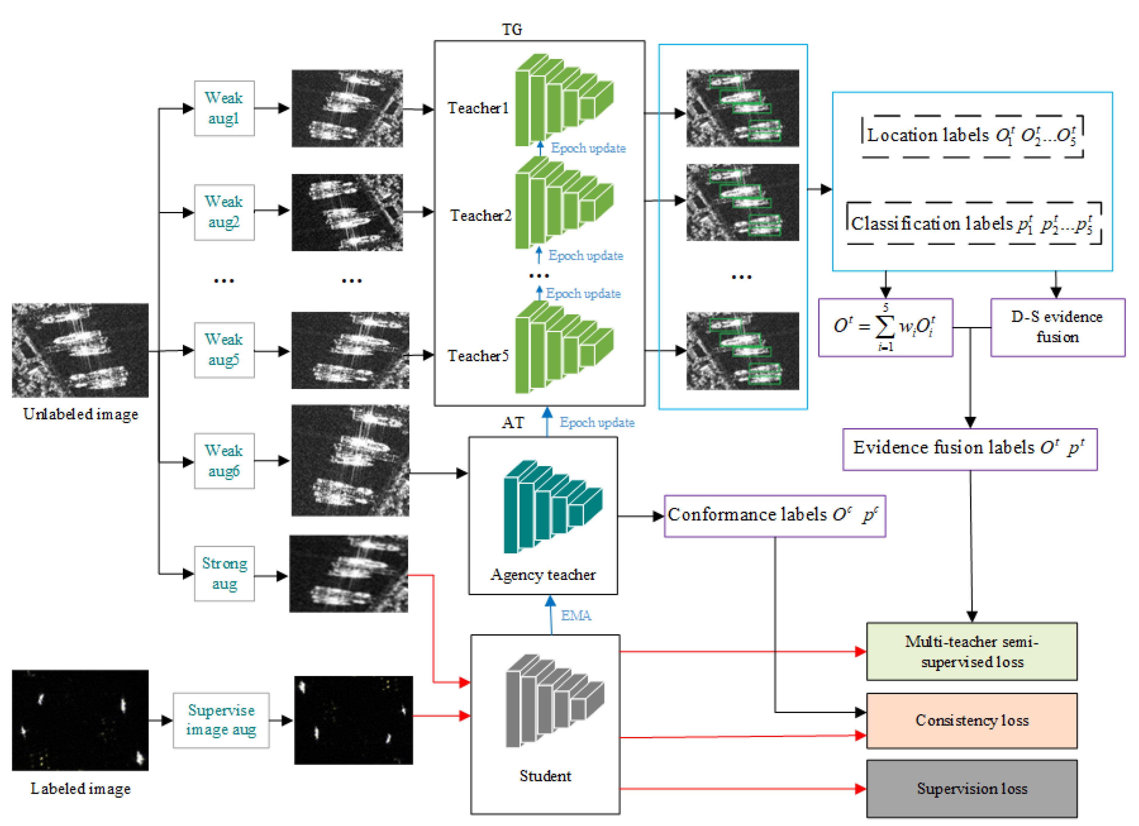
Figure 2.
Samples from the SSDD and AIR-SARShip-1.0 datasets. (a) SSDD; (b) AIR-SARShip-1.0.
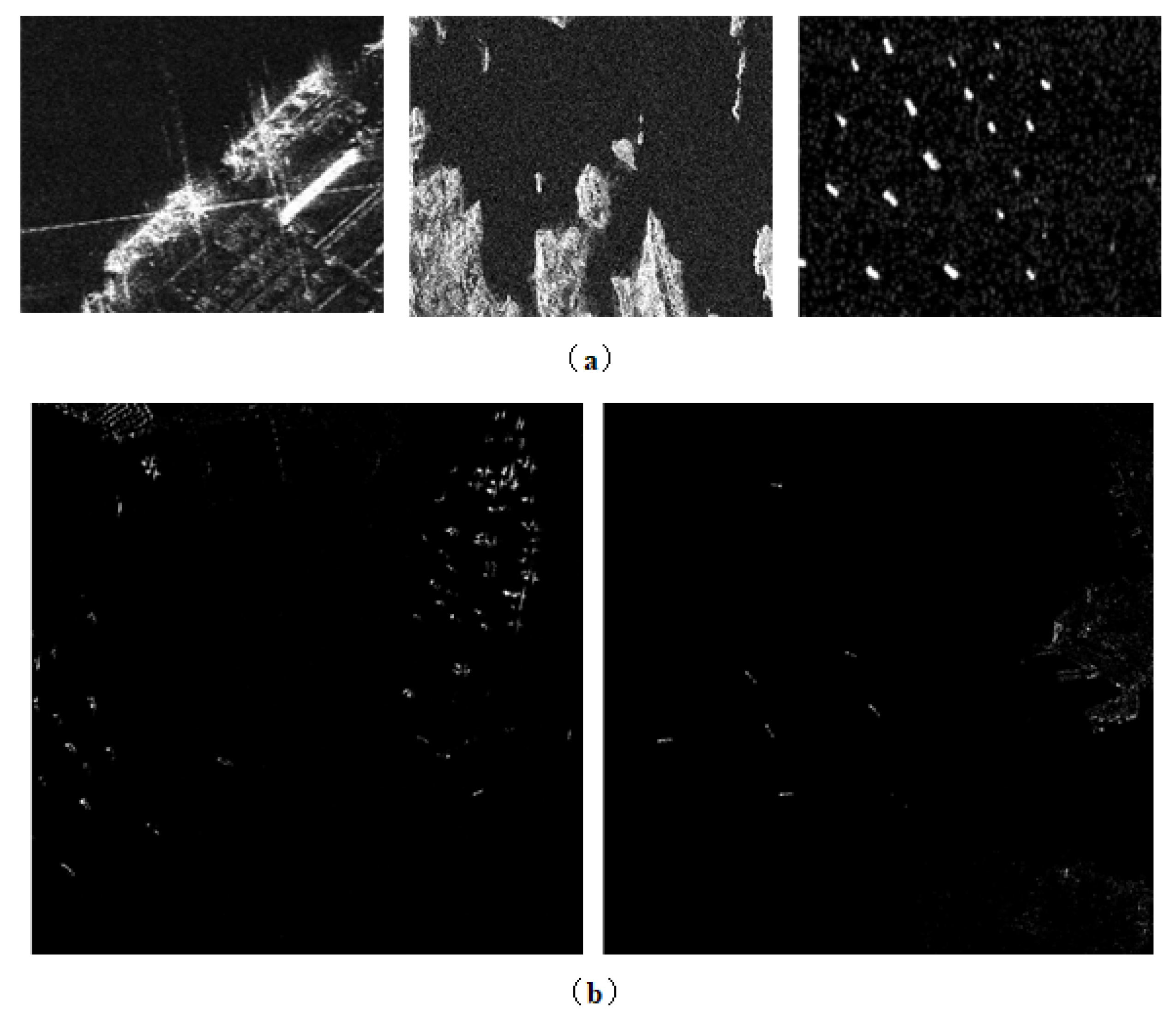
Figure 3.
The results of different algorithms on the SSDD dataset. From top to bottom, the results of Faster R-CNN, YOLOv8, Swin-Transformer, Soft Teacher, TSET, and Ours, are in that order. The green boxes denote all detected targets achieved by each algorithm. The red ellipses represent the false alarms identified by the algorithms. The orange ellipses denote missed instances that the algorithms failed to detect.
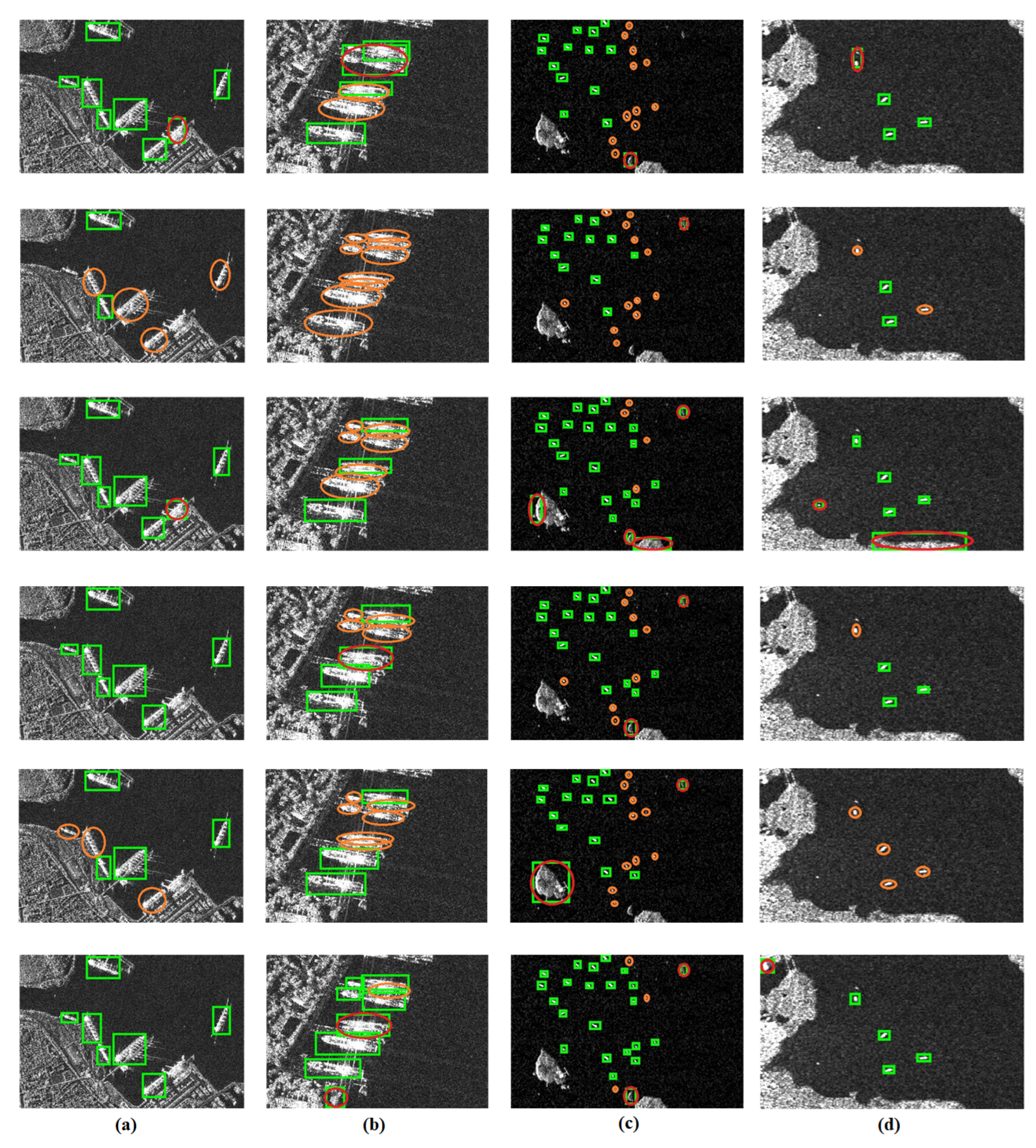
Figure 4.
pr curves for each algorithm on SSDD dataset
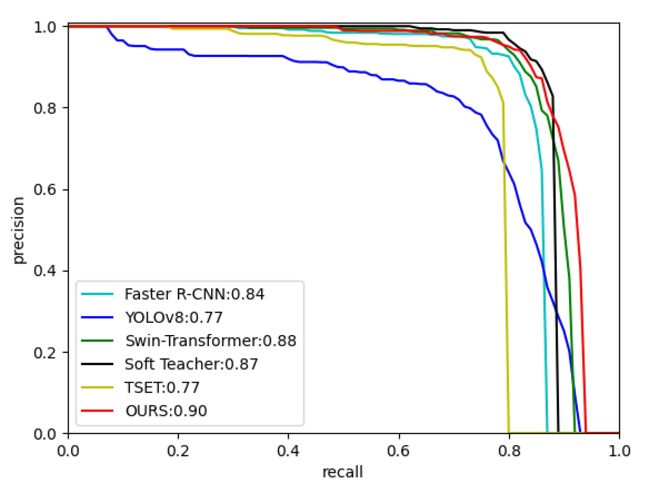
Figure 5.
The results of six algorithms on the AIR-SARShip-1.0 dataset. From top to bottom, the results of Faster R-CNN, YOLOv8, Swin-Transformer, Soft Teacher, TSET, and Ours, are in that order. The green boxes denote all detected targets achieved by each algorithm. The red ellipses represent the false alarms identified by the algorithms. The orange ellipses denote missed instances that the algorithms failed to detect.
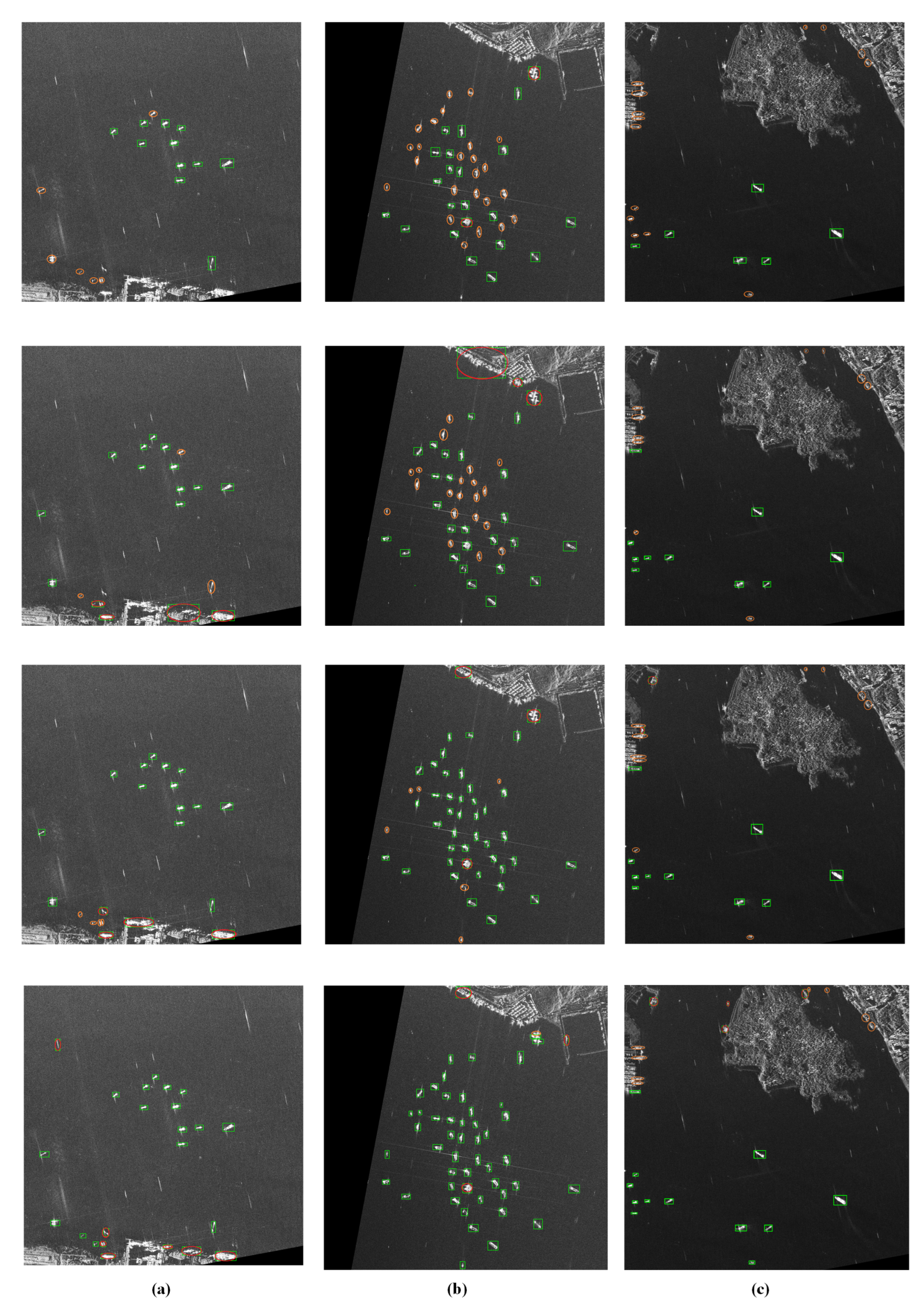
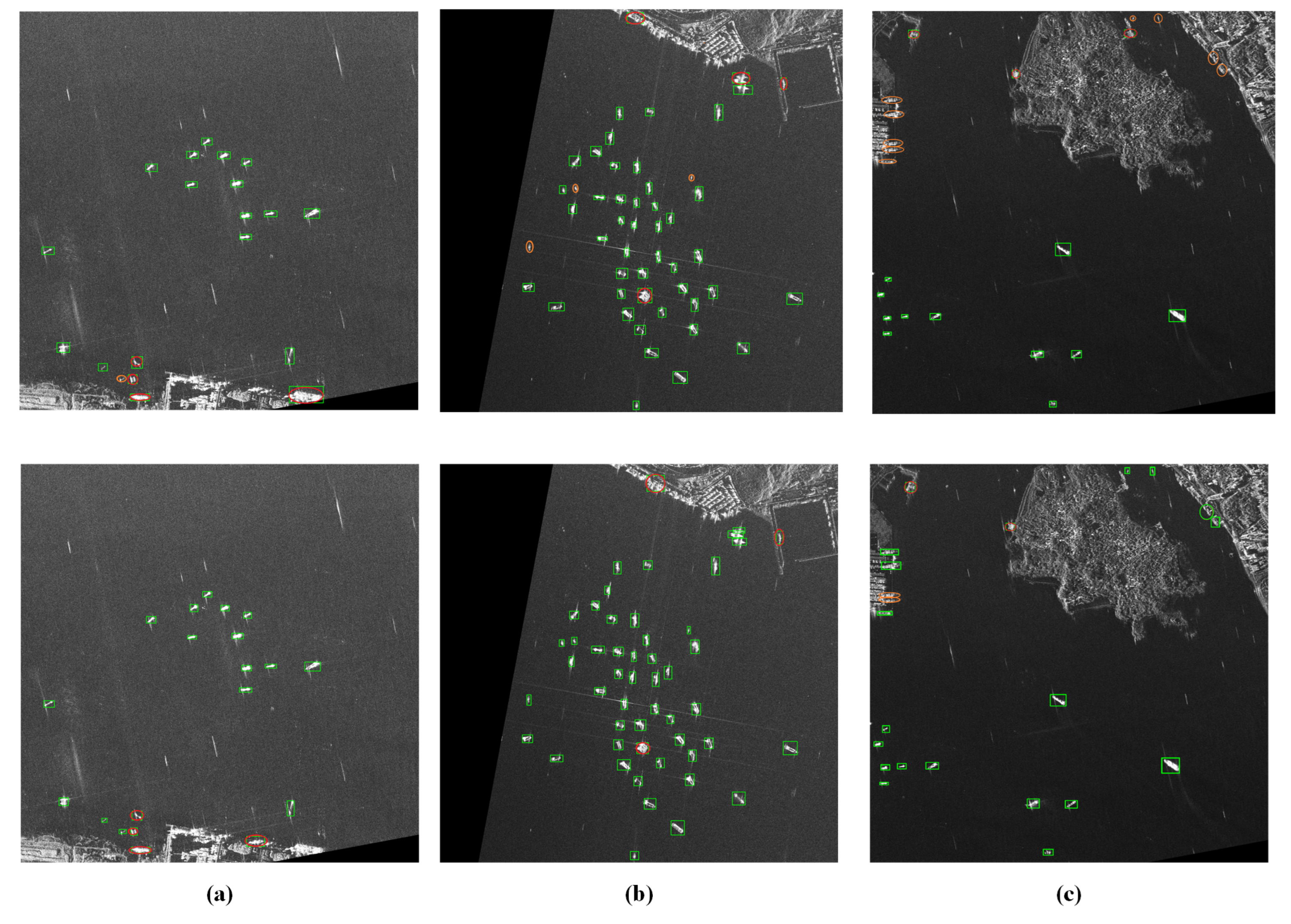
Figure 6.
pr curves for each algorithm on AIR-SARShip-1.0 dataset

Figure 7.
AP50 at different number of teacher
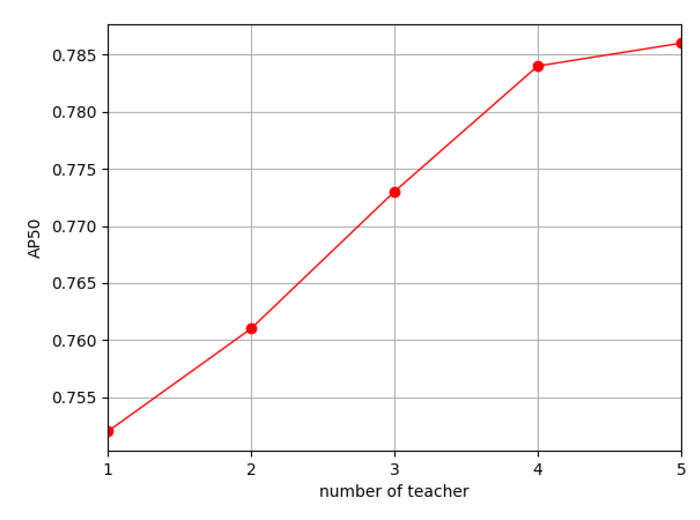
Figure 8.
Affects of .
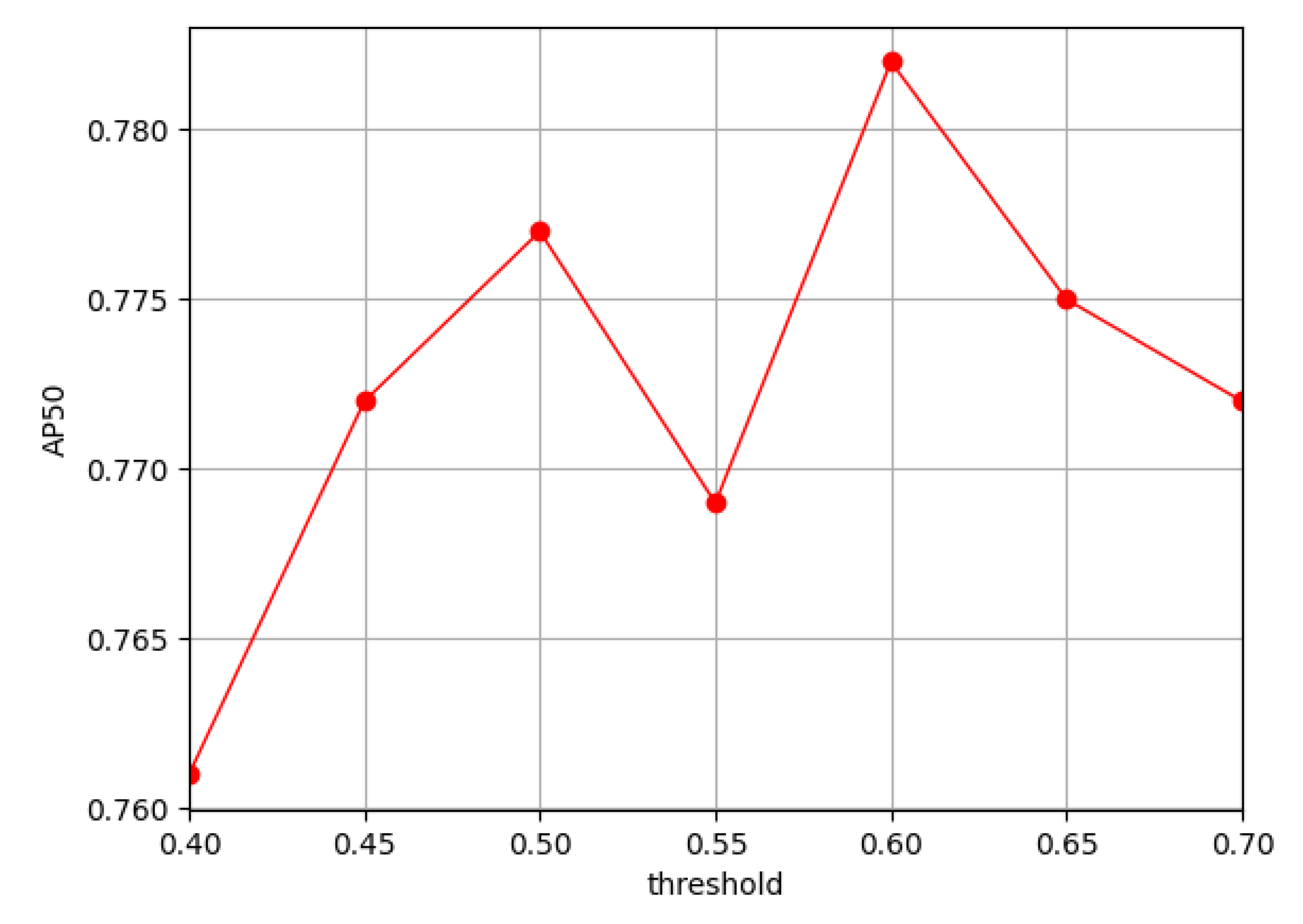

Table 1.
Specific information on the two datasets, SSDD and AIR-SARShip-1.0.
| Dataset | Sensors | Resolution | Polarization | Scenes |
|---|---|---|---|---|
| SSDD | RadarSat-2, TerraSAR-X, Sentinel-1 | 1m-15m | HH, HV, VV, VH | Nearshore, Offshore |
| AIR-SARShip-1.0 | Gaofen-3 | 1m, 3m | Single-Polarization | Ports, Islands, Various Sea Conditions |
Table 2.
COCO Metric.
| Metric | Meaning |
|---|---|
| AP | AP at IOU=0.50:0.05:0.95 |
| AP50 | AP at IOU=0.50 |
| AP75 | AP at IOU=0.75 |
| APS | AP for small object: area<322 |
| APM | AP for medium object: 322<area<962 |
| APL | AP for large object: 962<area |
Table 3.
COCO metrics on SSDD.
| Method | AP | AP50 | AP75 | APs | APm | APl |
|---|---|---|---|---|---|---|
| Faster R-CNN | 0.433 | 0.839 | 0.373 | 0.445 | 0.4 | 0.065 |
| YOLOv8 | 0.405 | 0.766 | 0.378 | 0.461 | 0.334 | 0.013 |
| Swin-Transformer | 0.464 | 0.878 | 0.412 | 0.484 | 0.396 | 0.153 |
| Soft Teacher | 0.437 | 0.868 | 0.340 | 0.435 | 0.454 | 0.392* |
| TSET | 0.415 | 0.769 | 0.365 | 0.422 | 0.403 | 0.151 |
| Ours | 0.498* | 0.905* | 0.461* | 0.504* | 0.483* | 0.23 |
* represents the best outcome.
Table 4.
COCO metrics on AIR-SARShip-1.0.
| Method | AP | AP50 | AP75 | APs | APm | APl |
|---|---|---|---|---|---|---|
| Faster R-CNN | 0.294 | 0.684 | 0.301* | 0.005 | 0.311 | 0.443 |
| YOLOv8 | 0.174 | 0.662 | 0.111 | 0.028 | 0.183 | 0.233 |
| Swin-Transformer | 0.291 | 0.681 | 0.175 | 0.047 | 0.303 | 0.454 |
| Soft Teacher | 0.35 | 0.776 | 0.232 | 0.023 | 0.363 | 0.463 |
| TSET | 0.34 | 0.764 | 0.219 | 0.024 | 0.356 | 0.450 |
| Ours | 0.351* | 0.793* | 0.233 | 0.097* | 0.363* | 0.524* |
* represents the best outcome.
Table 5.
COCO metrics of Ablation Study on AIR-SARShip-1.0.
| Multi-teacher | Ds Evidence Fusion | Agency Teacher | AP | AP50 | AP75 | APs | APm | APl |
|---|---|---|---|---|---|---|---|---|
| ✓ | ✗ | ✗ | 0.342 | 0.762 | 0.213 | 0.021 | 0.355 | 0.451 |
| ✓ | ✓ | ✗ | 0.349 | 0.770 | 0.257* | 0.143* | 0.359 | 0.508 |
| ✓ | ✗ | ✓ | 0.341 | 0.743 | 0.228 | 0.019 | 0.353 | 0.523 |
| ✗ | ✗ | ✓ | 0.35 | 0.776 | 0.232 | 0.023 | 0.363 | 0.463 |
| Ours | 0.351* | 0.793* | 0.233 | 0.097 | 0.363* | 0.524* | ||
* represents the best outcome.
Table 6.
impact on model performance.
| 0.01 | 0.05 | 0.1 | 0.5 | 1 | 2 | |
| AP50 | 0.779 | 0.793* | 0.788 | 0.786 | 0.773 | 0.75 |
* represents the best outcome.
Table 7.
impact on model performance.
| 0.1 | 0.25 | 0.5 | 0.75 | 1 | 1.5 | 2 | |
| AP50 | 0.773 | 0.785 | 0.784 | 0.768 | 0.793* | 0.775 | 0.764 |
* represents the best outcome.
Disclaimer/Publisher’s Note: The statements, opinions and data contained in all publications are solely those of the individual author(s) and contributor(s) and not of MDPI and/or the editor(s). MDPI and/or the editor(s) disclaim responsibility for any injury to people or property resulting from any ideas, methods, instructions or products referred to in the content. |
© 2024 by the authors. Licensee MDPI, Basel, Switzerland. This article is an open access article distributed under the terms and conditions of the Creative Commons Attribution (CC BY) license (http://creativecommons.org/licenses/by/4.0/).
Copyright: This open access article is published under a Creative Commons CC BY 4.0 license, which permit the free download, distribution, and reuse, provided that the author and preprint are cited in any reuse.
Downloads
108
Views
31
Comments
0
Subscription
Notify me about updates to this article or when a peer-reviewed version is published.


MDPI Initiatives
Important Links
© 2025 MDPI (Basel, Switzerland) unless otherwise stated