1. Introduction
COVID-19, caused by the SARS-CoV-2 virus, emerged as a significant global health threat in late 2019 [
1]. Identified initially in Wuhan, Hubei province of China, the disease quickly spread globally, leading the World Health Organization (WHO) to declare it a pandemic in March 2020. The virus’s origins have been the subject of extensive research, with studies suggesting that it likely jumped from an animal host, potentially bats, to humans, possibly with an intermediate host involved [
2]. The primary transmission mode is through respiratory droplets, although contact with contaminated surfaces can also result in infection [
3]. The disease manifests symptoms from mild cough and fever to severe respiratory distress, with older adults and those with underlying health conditions particularly vulnerable [
4]. COVID-19 has had profound global implications, affecting public health systems, economies, and daily lives. Efforts to combat its spread have included worldwide vaccination campaigns, the efficacy of which has been a primary focus of scientific research and public health initiatives [
5]. While there hasn’t been an approved vaccine or antiviral treatment for COVID-19, many countries and people have adopted non-pharmaceutical measures like wearing face masks in public, practising social distancing, and enforcing lockdowns to help curb the spread of the virus. [
6,
7]. Recent epidemiological research suggests that it’s important to consider the co-existence of COVID-19 and comorbidities like diabetes, lung disease, and heart disease. Individuals with these underlying conditions appear to have a heightened risk of contracting the virus [
8,
9]. Bjorgul, Novicoff and Saleh [
10] characterise comorbidities as diseases or medical conditions that coexist with the primary diagnosis under consideration while not sharing an origin or causal relationship. A mathematical model assessing the impact of comorbidity on COVID-19 dynamics, revealing that strategies preventing infection in individuals with comorbidities, particularly diabetes, are the most cost-effective as presented in [
32]. In line with the Centers for Disease Control and Prevention (CDC), individuals of any age with conditions such as chronic kidney disease, COPD (chronic obstructive pulmonary disease), a weakened immune state from a solid organ transplant, obesity (defined by a body mass index [BMI] of 30 or above), serious heart conditions like heart failure and coronary artery disease, Type 2 diabetes mellitus, hypertension or high blood pressure, and neurological conditions like dementia are at a heightened risk of experiencing severe complications from COVID-19 [
11]. A clinical study reported as [
12] further reinforces this understanding. In an examination of 41 confirmed COVID-19 patients, it was found that thirteen of them had pre-existing conditions such as hypertension, chronic obstructive pulmonary disease, cardiovascular disease, and diabetes. The transmission methods for infectious diseases have also been outlined in various studies, as indicated in [
13,
14].
In Nigeria, it has been observed that individuals with diabetes mellitus are more susceptible to contracting COVID-19. Studies suggest that those with severe COVID-19 symptoms have a higher incidence of diabetes mellitus than those with milder symptoms [
4]. The WHO recently cautioned that no conclusive evidence suggests that individuals who have recovered from COVID-19 are immune to a second infection [
15].
Models play a pivotal role in understanding the transmission dynamics of infectious diseases. The utilization of mathematical models for examining infectious diseases has seen a marked rise in recent periods, as indicated by studies [
16,
17]. Hence, the emergence of a branch has been done, which is called mathematical epidemiology. Frequent diagnostic tests, the availability of clinical data, and electronic surveillance have facilitated mathematical models’ applications to critically examine scientific hypotheses and design real-life strategies for controlling diseases [
18].
According to WHO, the COVID-19 vaccine is highly effective, but a small percentage of people will still get ill from COVID-19 after vaccination [
19,
20,
21]. Everybody could also pass the virus on to others who are not vaccinated. Mathematical models provided invaluable insights into potential transmission dynamics, peak infection times, and the potential impact of interventions [
22]. These models also identified key parameters like the basic reproduction number (R₀) and offered scenarios based on various containment strategies. The complexities surrounding COVID-19 transmission dynamics, co-infections, and their impact on global health have necessitated mathematical modelling as an essential tool in understanding and predicting disease trends [
23,
24,
25]. Recently, researchers have significantly contributed to the mathematical modelling of COVID-19 co-infections with other diseases.
Askari et al.[
26] , reported a groundbreaking understanding of the co-infections between COVID-19 and kidney disorders. It was observed that kidney disorders may exacerbate the progression of the COVID-19 disease. Dadashi et al. [
27] explored the co-infection rates of COVID-19 and influenza during the flu season. Mousquer et al. [
28] investigated the implications of co-infection of COVID-19 and tuberculosis in patients with compromised lung function.
Omame et al. [
16] conducted a study on co-infection transmission involving COVID-19 and diabetes in unvaccinated individuals. Hence, current research needs to address more comprehensively the intricacies of COVID-19 co-infections with diseases like diabetes. When juxtaposed with a contagious disease like COVID-19, many of these chronic and acute conditions offer a complex picture of public health. These interrelations, explored through mathematical models, have proved invaluable in shaping the global response and will continue to play a pivotal role in future public health crises.
This study investigates into the intricacies of these co-infections and will explore vaccination aimed at mitigating the severity and spread of the diseases. Therefore, conducting focused, comprehensive studies on these co-infections remains a crucial objective in our continued fight against the COVID-19 pandemic. A compartmental epidemic model with vaccination that cannot produce 100% immunity, analytical analysis of the model, numerical simulation, and discussions. This study explores the comparative dynamics of coronavirus disease with vaccination among individuals with or without comorbidity (diabetes mellitus).
2. Model Formulation
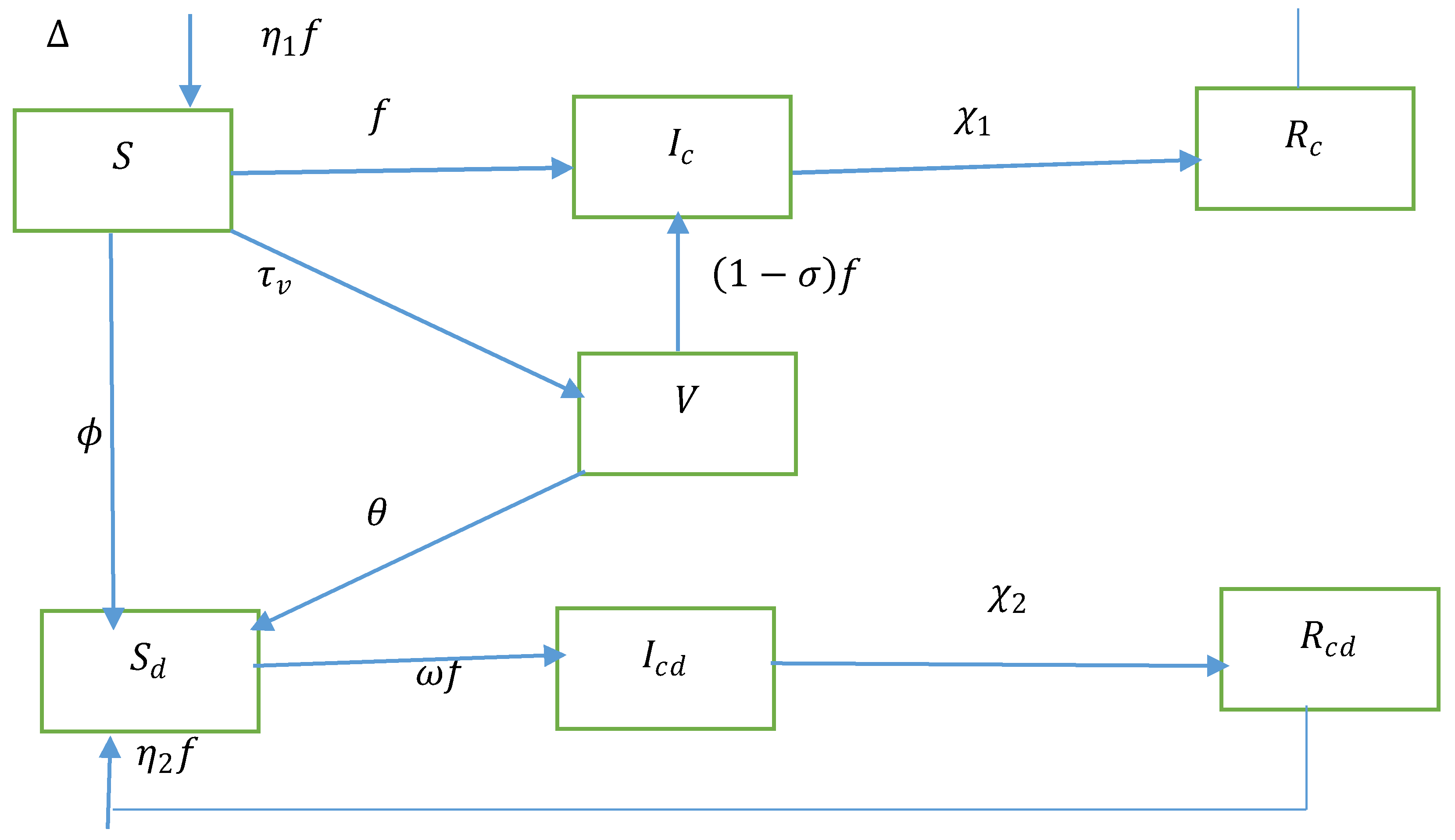
We delved into a seven-compartment model for a randomised human population. The entire group is split into seven distinct categories, namely susceptible population (S), COVID-19 infected, covid-19 vaccinated susceptible diabetic sensitive individualsCo infected Covid-19 and diabetics, Recover from Covid-19, Recover from Covid-19 but with people with diabetes.
We assumed that the recruitment increases the susceptible population at a rate. All populations in each compartment suffer from a natural death rate μ. The susceptible population (S) acquires COVID-19 at the rate where indicates the COVID-19 contact rate, Parameter alteration for higher infectiousness of co-infected persons due to comorbidity. Diabetes is becoming more common among people at this epidemiological rate at . Diabetes development rate in vaccinated susceptible persons. Vaccinated susceptible acquire COVID-19 at a decreased rate, where is the COVID-19 vaccine efficacy. COVID-19 vaccination rate from the susceptible populations. Diabetic susceptible acquire COVID-19 at the rate , where accounts for diabetics’ greater susceptibility rate. indicate recovery metrics for COVID-19 based on individual groupings and Covid-19 co-infected respectively. Reinfection rates for Individuals recovered from COVID-19 are in compartments and respectively.
Figure 1.
The transmission dynamics of diabetes and COVID-19 co-infection are shown in a flow chart.
Figure 1.
The transmission dynamics of diabetes and COVID-19 co-infection are shown in a flow chart.
Table 1.
Parameter description with values.
Table 1.
Parameter description with values.
| Parameter |
Biological Interpretation |
Value |
References |
|
Recruitment rate to susceptible populations |
630 |
calculated |
|
Vaccination rate COVID-19 (rate of people who are vaccinated) |
0.25 |
[4] |
|
COVID-19 contact rate |
1.2 |
Fitted |
|
Parameter alteration for higher infectiousness of co-infected persons due to comorbidity |
0.5776 |
Fitted |
|
COVID-19 vaccine efficacy |
0.70 |
[3] |
|
The compartment indicates the reinfection rates for individuals recovered from COVID-19. |
0.0013 |
Estimated |
|
The compartment indicates the reinfection rates for individuals recovered from COVID-19. |
0.0013 |
Estimated |
|
Accounts for diabetics’ greater susceptibility rate. |
0.60 |
[1] |
|
Rate of Diabetes development for susceptible humans |
0.0028 |
Estimated |
|
Diabetes increased rate in vaccinated susceptible persons |
0.018 |
Fitted |
|
Recovery rates for COVID-19 within the compartment. |
0.00014 |
Fitted |
|
Recovery rates for COVID-19 within the compartment. |
0.0124 |
Fitted |
|
Natural death rate |
|
calculated |
Theorem 1. All the populations of the system with positive initial conditions are nonnegative let
, then
of the system are positive for all time
.
By using the technique of variable separation
can be reduced to
Then, the above equation is integrated to yield the solution below
Since the initial value, and the exponential functions in equation (8) are always positive
Hence,
is positive. Using a similar technique to verify other equations of equations (1) to (7), this shows that
Theorem 2. The dynamical system (1) to (7) is positively invariant in the closed invariant set
To obtain an invariant region that shows that the solution is bounded, we have
The general solution of the equation
, where
We can follow that
as
Thus, it can be concluded that
is boundedas
Hence, the feasible region of the model in the nonnegative region is defined as
3. Analytical Analysis of Co-Infection Model
We compute the equilibrium and provide conditions for their existence. We also determine the reproduction number of the model and use it to study the stability of the computed equilibria and the sensitivity of the model.
3.1. The Disease-Free Steady-State Equilibrium Points of the Model
The disease-free equilibrium of equations (1) to (7) are given by
Hence, the disease-free equilibrium point (DFEP) of the COVID-19 co-infection model is
3.2. The Basic Reproduction Number
The largest eigenvalue is the basic reproduction number.
3.3. Stability Analysis at Disease-Free Equilibrium Point
The disease-free equilibrium is locally asymptotically stable if , and unstable if .
Jacobian matrix of the system (1) to (7)
At the disease-free equilibrium point
where,
, and the solution of
Polynomial characteristic
Utilising the Routh-Hurwitz criterion, if , equation (12) will only have roots with negative real parts. Consequently, the disease-free equilibrium J is locally stable when .
3.4. Endemic Equilibrium Analysis
For the equilibrium points of the equations (1) to (7),
Let ,
represents the disease equilibrium point. The components of
are the positive solutions of the nonlinear system of equations
Theorem 3. The endemic equilibrium point is locally stable when the basic reproduction number.
3.5. Global Stability of DFE and the EE Point
At the COVID-19 free equilibrium point (CFE) we have the following form
Hence,
if and only if
. Therefore, L is a Lyapunov function for the system (1) to (7). It follows by the La Salle’s Invariance Principle [
24], that the CFE of the model (1) to (7) are globally
The lyapunov function is defined as
The function
needs to be proven to determine whether the Lyapunov function is valid or invalid for
It is proven that
Because
, so that it is showed that
.
Now,Based on the description above, it can be concluded that if and if . Hence, by LaSalle’s invariance principle, it means that the endemic equilibrium point in the spread o fCOVID-19 is globally asymptotically stable if R0>1.
3.6. Sensitivity Analysis
The sensitivity index quantifies the relative variation in a state variable in response to a parameter modification and is determined using sensitivity analysis. Using the method developed by Chitnis et al. [
28], we calculate the sensitivity indices of
to the model parameters. These indices highlight the significance of each aspect in the dynamics and prevalence of disease transmission. Sensitivity analysis is used to identify the most relevant elements that impact the community’s ability to contain and spread infection. We apply the technique offered to do sensitivity analysis.
The sensitivity indices in
Table 2 are described as follows: for parameters with positive indices, the corresponding basic reproduction number increases (decreases) as those parameters increase (decreases). On the other hand, negative indices suggest that as those parameters increase, the associated basic reproduction number decreases, and vice versa. According to
Table 2, 10% increase or reduction of
causes 10% increase or reduction in the value of
, 10% increase or reduction of
causes 10 % increase or decrease in the value of
, 10% increase or reduction of
causes 1.1% increase or decrease in the value of
, 10% increase or reduction of
causes 1.6% reduction or increase in the value of
, 10% increase or reduction of
causes 10% reduction or increase in the value of
, 10% increase or reduction of
causes 9.4 % reduction or increase in the value of
, and 10% increase or reduction of
causes 4.2 % reduction or increase in the value of
.
Sensitivity analysis was conducted using the partial rank correlation coefficients (PRCCs) combined with the Latin hypercube sampling to assess the influence of each model parameter on the initial spread of the disease, represented by
.
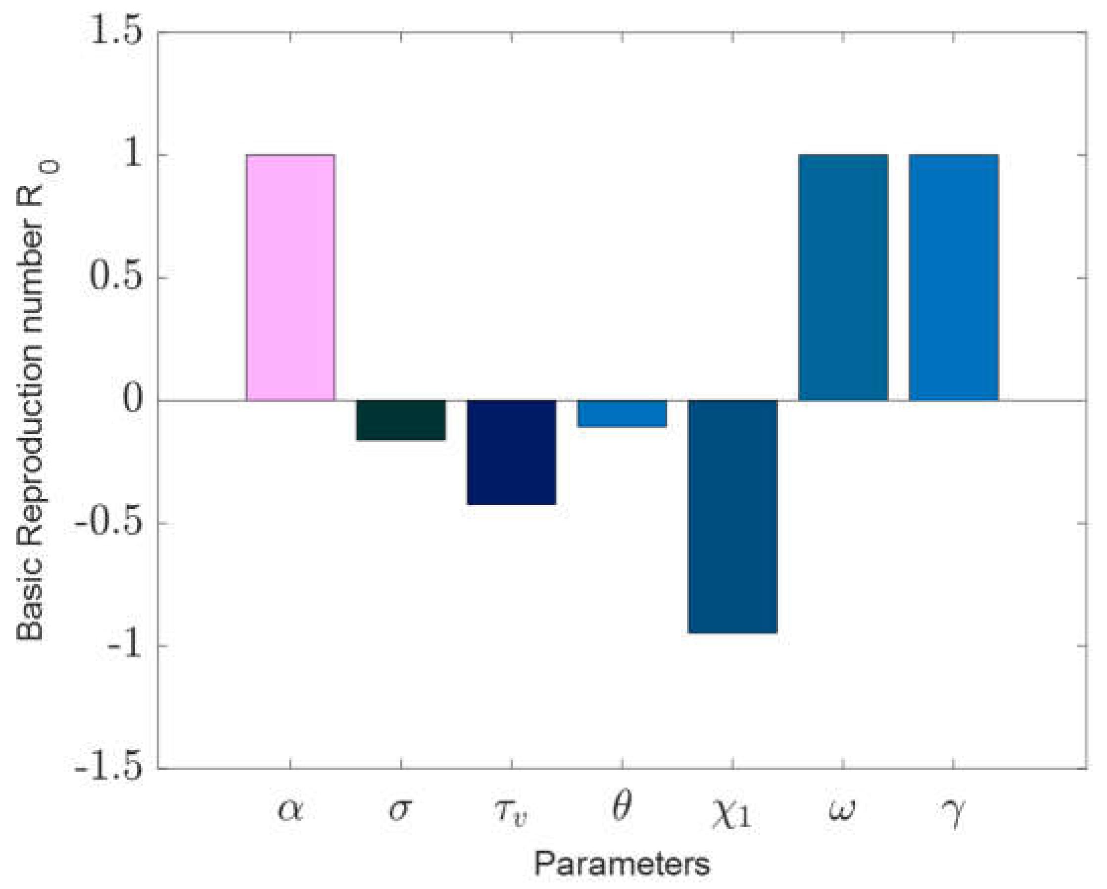
Figure 2 illustrates the PRCCs, highlighting the ramifications of altering input parameters on the basic reproduction number,
. Parameters that have positive PRCCs enhance the initial transmission rates, whereas those with negative PRCCs curtail
A closer look at
Figure 2 helps pinpoint the most impactful parameters.
Table 2’s sensitivity indices reveal that when the values of α, ω, and γ surge, and other parameters remain constant, there’s an uptick in
suggesting increased disease endemicity due to the positive indices. Conversely, when the parameters
and
drop and other values remain unchanged,
diminishes, indicating a decline in disease endemicity given the negative indices. The contact rate
and the higher infectiousness of the co-infected person’s rate
are the most sensitive parameters.
3.7. Data Fitting and Parameters
The population of Bangladesh, as cited in source [
26], is approximately 170000000. Additionally, referencing a study by Dahiru et al. [
29], which investigated the prevalence of diabetes mellitus in Bangladesh, we set specific initial conditions in our analysis of COVID-19 in the region. Considering the first infected in Bangladesh, we try to explore the dynamics of worldwide daily and cumulative cases from April 2020. The data is retrieved from the World Health Organization (WHO) ‘s website [
26]:
= 0.93 * 170000000: This represents the initial number of susceptible individuals without comorbidities, calculated as 93% of the total population.
) = 0.07 * 1700000: This denotes the initial number of susceptible individuals with comorbidities at 7% of the total population.
= 412320: This indicates the initial number of COVID-19 cases without comorbidities.
) = 0: This is the initial number of recovered individuals from COVID-19 without comorbidities.
: This signifies the initial number of COVID-19 cases with comorbidities.
= 0: This represents the initial number of recovered individuals from COVID-19 with comorbidities. In our analysis, two optimisation algorithms were utilised for data fitting purposes. The objective function is root mean error square
.The first was the genetic algorithm (GA), and the second was the fmincon algorithm, as documented in references [
30,
31].
This led to the calculation of the natural mortality rate per month as the inverse of life expectancy, resulting in a value of
. Furthermore, the recruitment rate was approximated by manipulating the ratio of
to yield the initial population, resulting in
individuals per day. Due to limited data on co-infections, we estimated certain co-infection-related parameters, while others were deduced from actual data. During the estimation process, the initial conditions of the state variables were set as delineated in
Table 1.
The
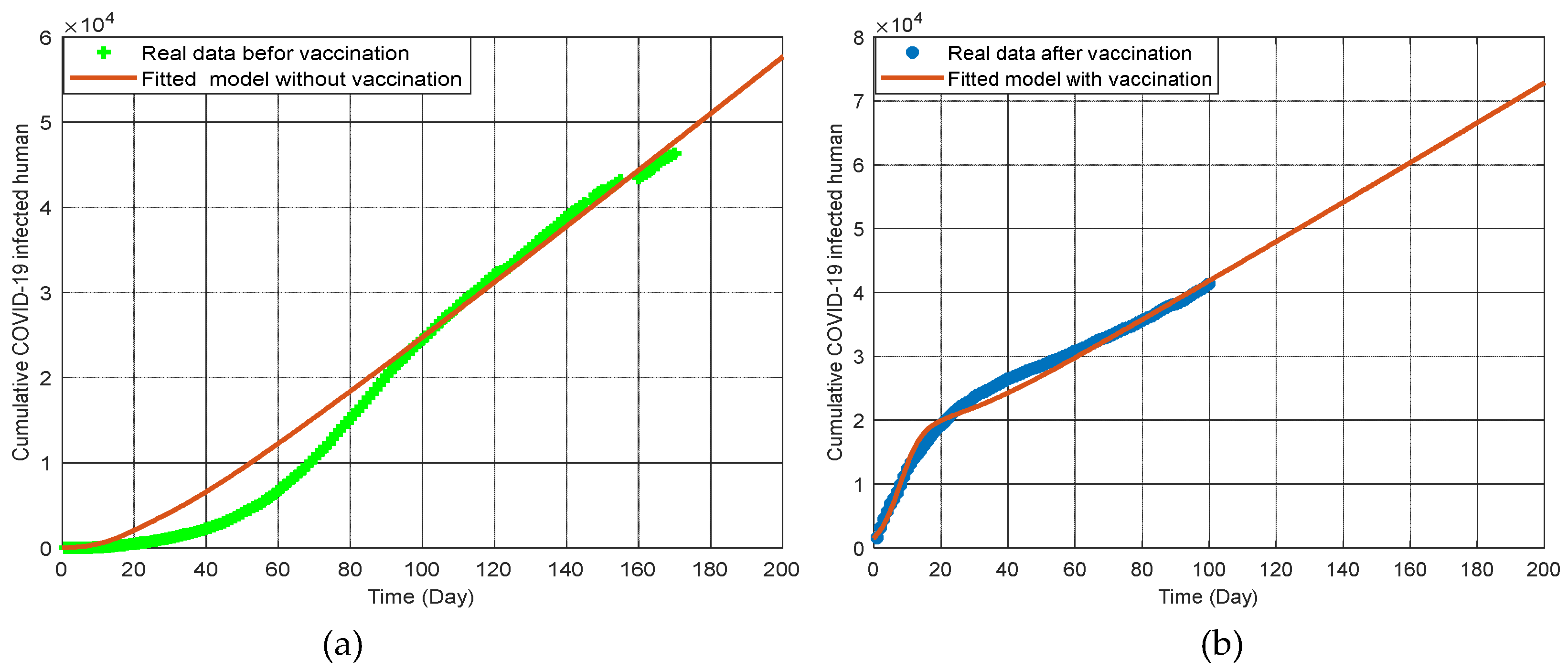
Figure 4(a) represents the cumulative COVID-19 infected population from April 2020 to October 2020 [
26]. This period captures data before the implementation of COVID-19 vaccinations. The green dots indicate the real data collected during this time frame, while the brown line represents the fitted model without vaccination. The graph shows a clear increase in the number of COVID-19 cases, reflecting the natural progression of the pandemic before any vaccination measures were in place. The close fit between the model and the real data demonstrates the model’s accuracy in predicting the spread of COVID-19 in the absence of vaccinations.
The graph 4(b) represents the cumulative COVID-19 infected population from September 2021 to April 2022 [
26], which covers the period after the implementation of COVID-19 vaccinations. The blue dots indicate the real data collected during this period, and the brown line represents the fitted model with vaccination. This graph shows a significant change in the infection trend compared to the pre-vaccination period. The data indicates that vaccination has played a crucial role in reducing the number of new infections and controlling the spread of the virus. The fitted model closely aligns with the real data, highlighting the model’s effectiveness in capturing the impact of vaccination on the COVID-19 pandemic.
These graphs collectively illustrate the dramatic difference in COVID-19 infection trends before and after vaccination. The pre-vaccination period saw a steady rise in infections, accurately captured by the model. In contrast, the post-vaccination period shows a controlled infection rate, demonstrating the critical role of vaccination in managing and reducing the spread of COVID-19. These findings underscore the importance of vaccination campaigns in mitigating the impact of the pandemic and provide valuable insights for public health strategies in regions like Bangladesh. Additionally, the data shows that increasing vaccination rates not only decrease the number of COVID-19 cases but also reduce the incidence of co-infections with comorbidities, thereby improving overall public health outcomes. This highlights the dual benefit of vaccinations in controlling the pandemic and managing chronic health conditions.
4. Numerical Result and Discussions
The model’s analytical outcomes can be visualized through numerical simulations using parameter values sourced from existing literature. For system analysis, the ODE113 solver from MATLAB is utilized. A simulation of the Co-infection Model is carried out in vaccination treatments to examine how the key determinants may affect the transmission of COVID-19 in diabetics and non-diabetics. The Co-infection Model following vaccine interventions has a disease-free equilibrium that is locally asymptotically stable when the related effective reproduction number, is available. COVID-19 would be removed from the population if the initial conditions shifted toward the disease-free equilibrium point. Based on the findings, it can be believed that only the COVID-19 recovery rate will improve with immunization.
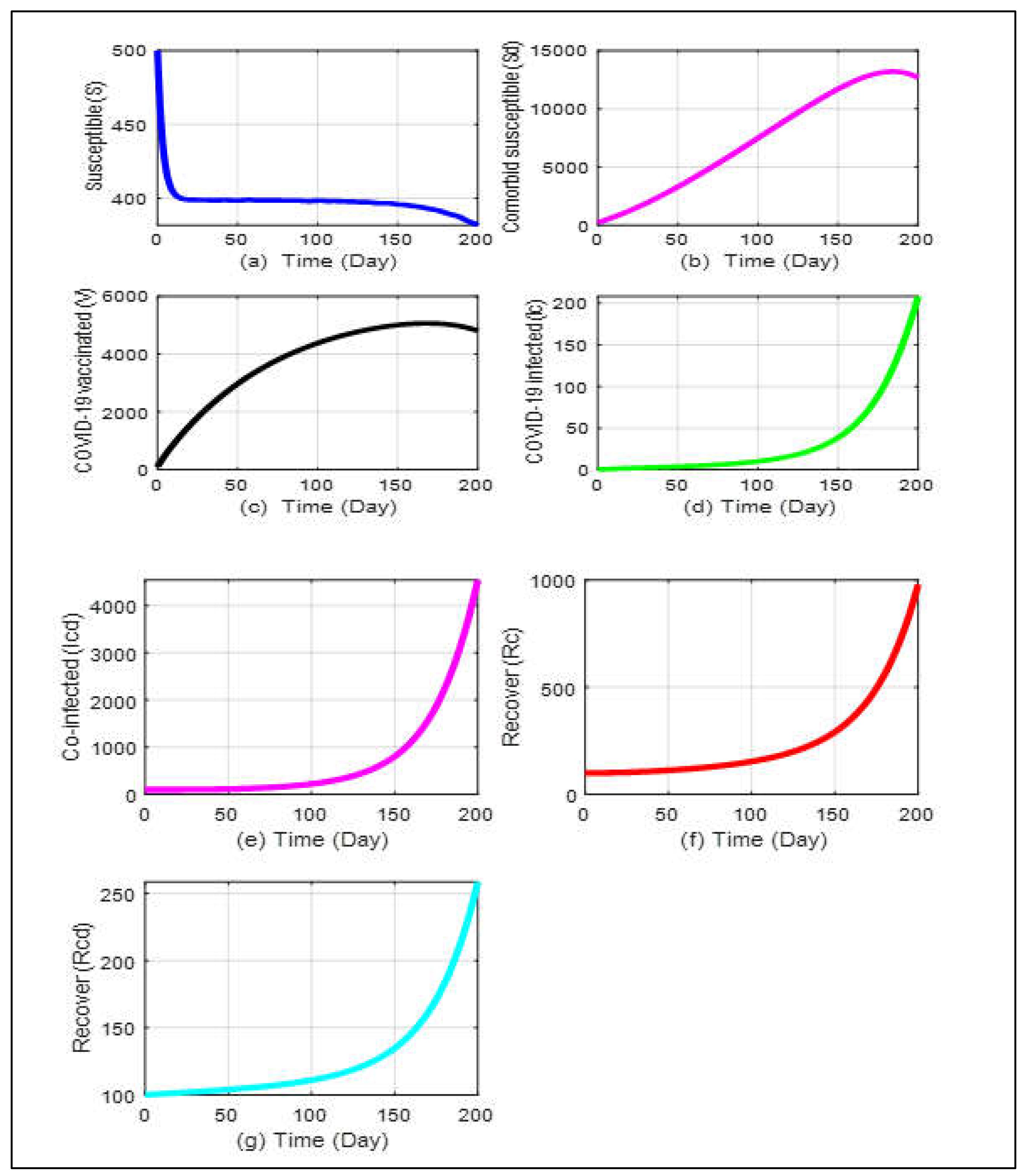
From
Figure 5a,b, we see that the susceptible people are monotonically declining. At the same time, the number of comorbid susceptible people initially keeps rising, but after a few days, it gradually falls. In
Figure 5d,e, since the start of this pandemic, the COVID-19 infected curve and the co-infected curve have progressively climbed, but after a few days, both curves have unexpectedly increased as well. On the other hand, the COVID-19 vaccination rate presented in
Figure 5c is also higher than the recovery rate for people mentioned in
Figure 5f,g. According to the graph’s dynamic nature, it is predicted that until a vaccination or appropriate treatment is introduced, the sick people will continue to develop. Even yet, it can be managed by preserving physical distances, raising the vaccination rate, and creating a self-immunity system, as revealed by our study. We run the program keeping all other values of the parameters same as before for infected and Co- infected individuals.
The simulation’s outcome under these conditions is depicted in
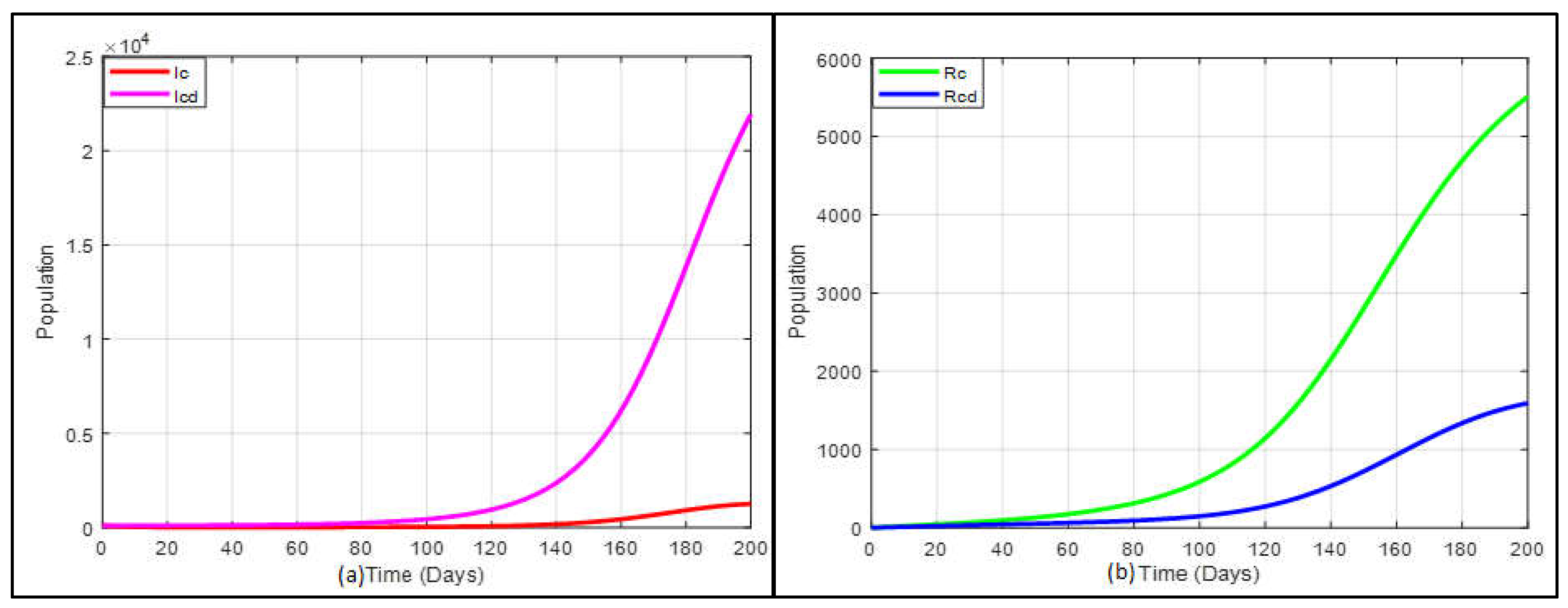
Figure 6a which indicates that the predicted total number of inpatients co-infected with COVID-19 and diabetes is more rapidly increased than only the COVID-19-infected population if the vaccination strategy is not executed. The expected total number of inpatients, only those with COVID-19, is more swiftly increased recovered than those co-infected with COVID-19 and diabetes population when the vaccination strategy is not applied, which is presented in
Figure 6b.
In epidemiology, disease spread and persistence are closely tied to the basic reproduction number and the endemic equilibrium point. This reproduction number is a marker for the initial dissemination of an ailment among a susceptible population, quantifying the average number of follow-on infections from a singular infected person introduced to a previously uninfected group. The spread of the coronavirus will diminish if
is under 1, but will sustain if
is above 1. To identify the key parameters affecting the coronavirus transmission, we ran a program using initial and parameter values detailed in Tab.1. The outcomes from this analysis are captured in
Figure 6,
Figure 7,
Figure 8 and
Figure 9.
Figure 7,
Figure 8,
Figure 9 and
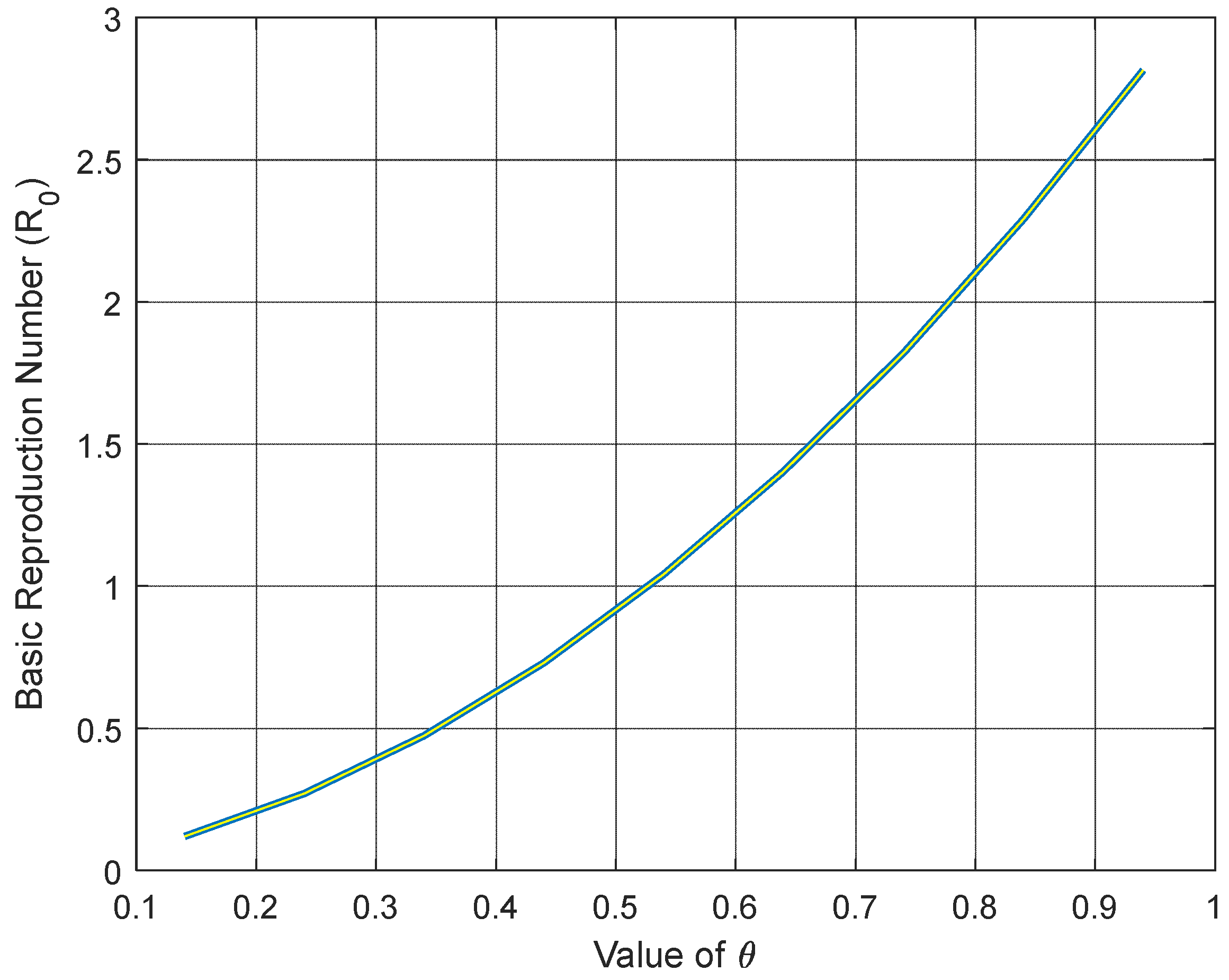
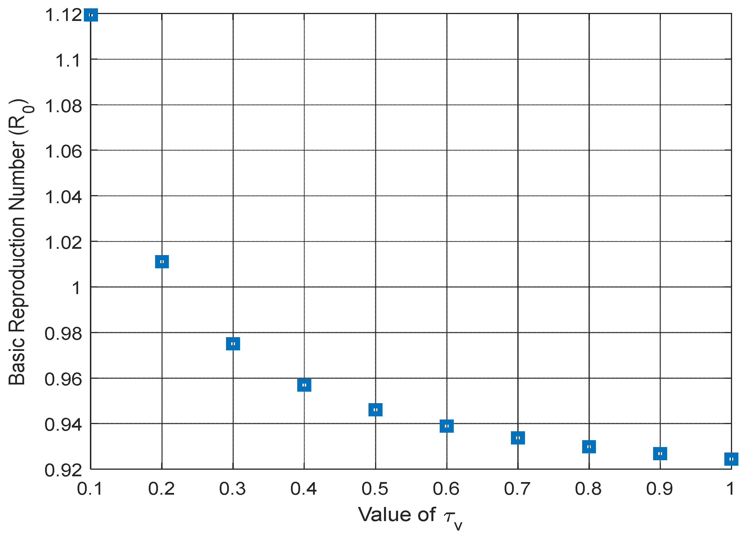
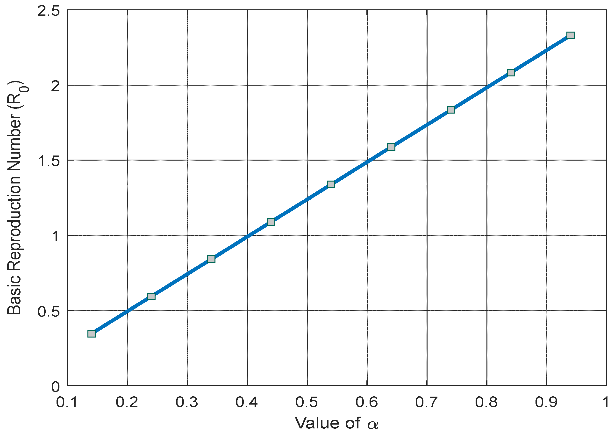
Figure 10 illustrate how the basic reproduction number changes in relation to key parameters that influence the ongoing pandemic. Specifically,
Figure 7 indicates that as the rate of diabetes (θ) rises in vaccinated susceptible individuals, the basic reproduction number surges exponentially, suggesting the disease’s continued presence in the community.
Figure 8 and
Figure 9 highlight a significant reduction in the basic reproduction number when considering the COVID-19 vaccine’s efficacy rate (σ) and the growth in the vaccination rate (
). Meanwhile,
Figure 10 depicts a linear increase in the basic reproduction number as the COVID-19 contact rate (
) climbs.
The Influence of Vaccination
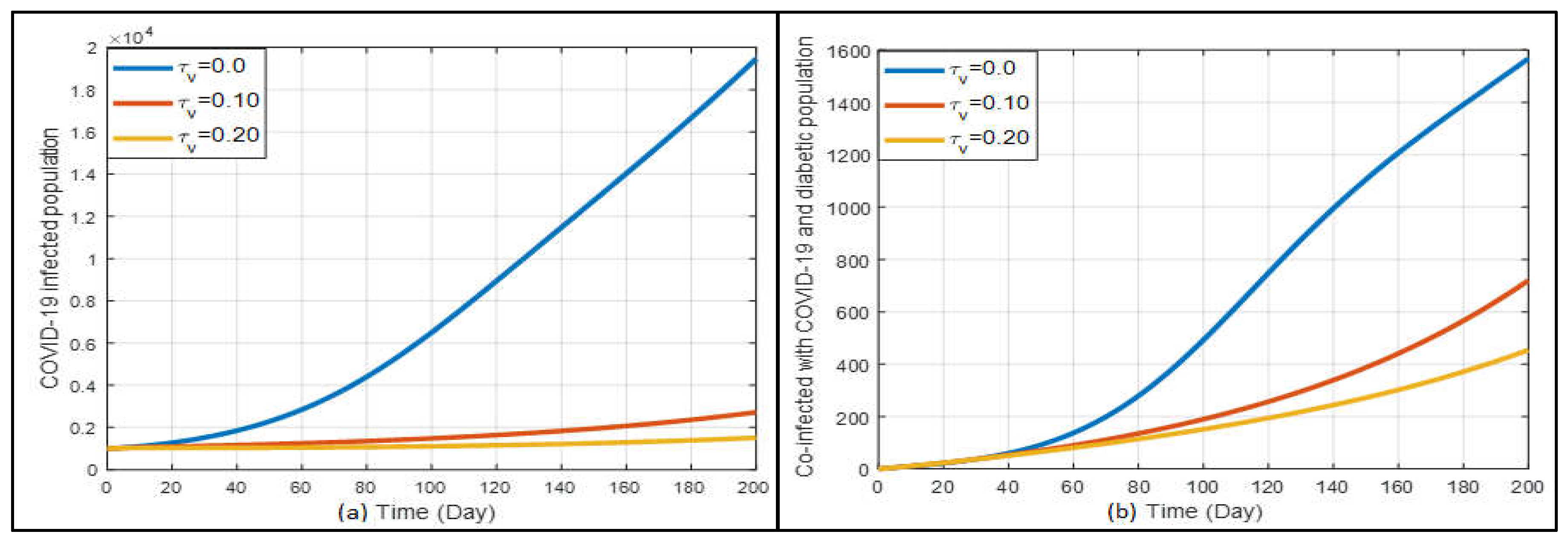
Figure 11a shows the results related to the effects of vaccination. When
is 0, it means there is no vaccination taking place. From the current data, it seems that our rate of vaccination isn’t drastically reducing the number of COVID-19 cases. However, when we look closer at
Figure 11a, as more people get vaccinated, the number of infections starts to drop slowly. It is interesting to note that for people with diabetes, COVID-19 cases still rise a bit even with a moderate vaccination rate
). But, when more people are vaccinated at a higher rate (
), the number of infections reduces, which is also shown in
Figure 11b.
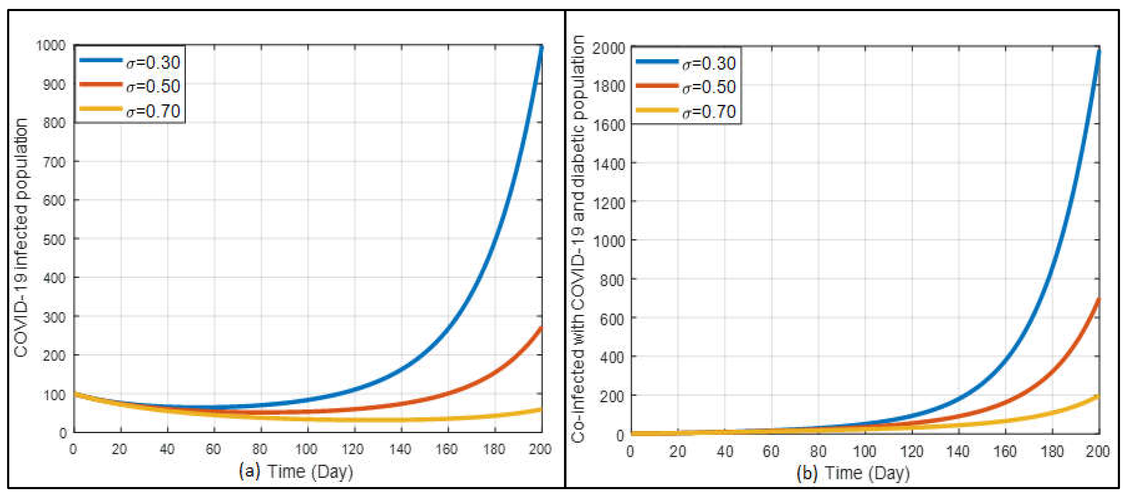
The vaccine’s efficacy is also a vital factor in eliminating the disease. In
Figure 12a shows a marked reduction in the number of COVID-19-infected cases as the vaccine efficacy increases. With higher vaccine efficacy (σ=0.70), the infection rate significantly decreases, demonstrating the vaccine’s crucial role in controlling the pandemic. This suggests that effective vaccination campaigns can substantially mitigate the spread of COVID-19. On the other hand, the graph 12(b) illustrates that higher vaccine efficacy also reduces the number of co-infected cases of COVID-19 and diabetes. Over a long-term period, as vaccine efficacy increases, the incidence of co-infection decreases. This underscores the importance of high-efficacy vaccines in protecting diabetic patients, who are more vulnerable to severe outcomes.
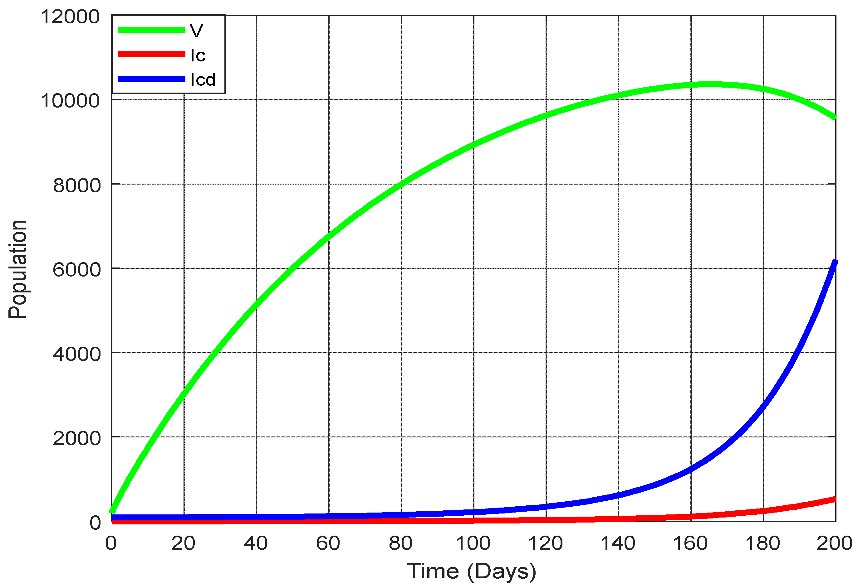
Figure 13 displays the changing trajectories for three states: vaccination, COVID-19 infection, and co-infection with COVID-19 and diabetes. Notably, as the rate of vaccination rises, there’s a marked decrease in the number of individuals infected with COVID-19 and those co-infected with both the virus and diabetes. But when the vaccination rate is decreasing, the infected population and co-infected with COVID-19 and diabetes are increasing.
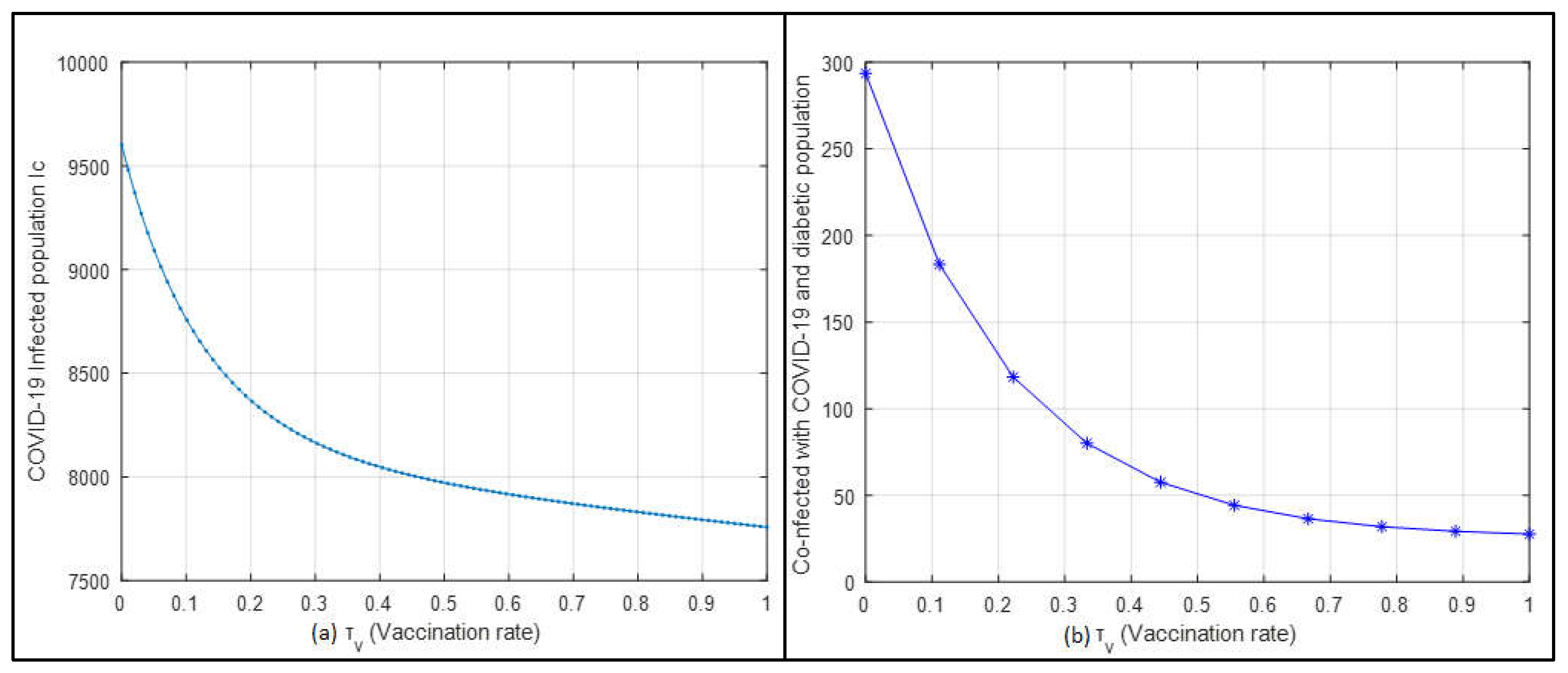
In
Figure 14a, the relationship between the vaccination rate and the COVID-19-infected population is depicted. As the vaccination rate increases, there is a noticeable decline in the number of individuals infected with COVID-19. This highlights the effectiveness of increasing vaccination rates in controlling and reducing the spread of the virus. Similarly,
Figure 14b shows an inverse relationship between the vaccination rate and the co-infected population with COVID-19 and diabetes. As vaccination rates rise, the number of co-infected individuals significantly decreases. These figures clearly demonstrate that higher vaccination rates effectively reduce the spread of COVID-19 and its co-infections. The marked reduction in both COVID-19 cases and co-infections with increased vaccination underscores the crucial role of vaccination in disease control.
5. Conclusions
We crafted a mathematical framework to assess the influence of vaccination on individuals co-infected with COVID-19 and diabetes. The study emphasized how the spread of COVID-19 has significant adverse effects on public health. We further investigated the impact of vaccination on the effectiveness of infection on the co-infection of COVID-19 and diabetes. Moreover, the critical vaccination threshold is derived, and it is underlined that even if a significant proportion of the population obtains vaccination. The following list includes the main conclusions of the new development model:
An increased rate of transmission significantly impacts the disease’s spread.
A reproduction number less than one could lead to a disease-free equilibrium, making it globally unstable.
The importance of the critical vaccination threshold was highlighted. Even high vaccination rates might not eliminate the disease if vaccine efficacy and disease reproduction are low.
Vaccinations have been empirically reduce disease spread successfully.
A significant inverse relationship was observed in our study between the vaccination rate and the incidence of both COVID-19 and its co-infections with diabetes.
While co-infections were evident, the severity or complexity of the co-infection between COVID-19 and diabetic complications remained consistent, without any observed intensification.
The findings reached through the sensitivity analysis are aligned with the observations made using the model, with a specific emphasis on how crucial transmission affects the progress of the disease. The findings support broad COVID-19 vaccination drives begun by the government, with a focus on diabetics. The current findings and models also maximise the advantages of simulation modelling to reduce COVID-19 and diabetes disease’s global health complexity. Research directions in the future can concentrate on the effectiveness of different vaccination doses among various human races.
Author Contributions
Md. Abdul Hye and Md. Haider Ali Biswas: conceptualization, formal analysis, software, and original draft preparation. Md. Abdul Hye and Mohammed Forhad Uddin: methodology. Mohammed Forhad Uddin and Md. Haider Ali Biswas: validation and investigation and resources. Md. Abdul Hye: data curation. Mohammed Forhad Uddin: review and editing. Mohammed Forhad Uddin and Md. Haider Ali Biswas: supervision. All the authors have read and agreed to the published version of the manuscript.
Data Availability Statement
Data will be available upon request.
Acknowledgments
We would like to express our endless gratitude to Bangladesh University of Engineering and Technology (BUET) primary research fund for its continuous logistic and financial support and valuable insights during this research.
Conflicts of Interest
The authors declare that there are no conflicts of interest regarding the publication of this manuscript.
References
- W.H. Organization, World Health Organization coronavirus disease (COVID-19) dashboard, World Health Organization, (2020).
- P. Zhou, X.-L. Yang, X.-G. Wang, B. Hu, L. Zhang, W. Zhang, H.-R. Si, Y. Zhu, B. Li, C.-L. Huang, Addendum: A pneumonia outbreak associated with a new coronavirus of probable bat origin, Nature, 588 (2020) E6-E6.
- M. Nicola, Z. Alsafi, C. Sohrabi, A. Kerwan, A. Al-Jabir, C. Iosifidis, M. Agha, R. Agha, The socio-economic implications of the coronavirus pandemic (COVID-19): A review, International journal of surgery, 78 (2020) 185-193. [CrossRef]
- A. Egonmwan, D. Okuonghae, Mathematical analysis of a tuberculosis model with imperfect vaccine, International Journal of Biomathematics, 12 (2019) 1950073.
- F.P. Polack, S.J. Thomas, N. Kitchin, J. Absalon, A. Gurtman, S. Lockhart, J.L. Perez, G. Pérez Marc, E.D. Moreira, C. Zerbini, Safety and efficacy of the BNT162b2 mRNA Covid-19 vaccine, New England journal of medicine, 383 (2020) 2603-2615.
- P. Van den Driessche, J. Watmough, Reproduction numbers and sub-threshold endemic equilibria for compartmental models of disease transmission, Mathematical biosciences, 180 (2002) 29-48. [CrossRef]
- C.M. Gomes, L.A. Favorito, J.V.T. Henriques, A.F. Canalini, K.M. Anzolch, R.d.C. Fernandes, C.H. Bellucci, C.S. Silva, M.L. Wroclawski, A.C.L. Pompeo, Impact of COVID-19 on clinical practice, income, health and lifestyle behavior of Brazilian urologists, International braz j urol, 46 (2020) 1042-1071.
- A. Azeez, J. Ndege, R. Mutambayi, Y. Qin, A mathematical model for TB/HIV co-infection treatment and transmission mechanism, Asian J. Math. Computer Res, 22 (2017) 180-192.
- H. Tasman, An optimal treatment control of TB-HIV coinfection, International Journal of Mathematics and Mathematical Sciences, 2016 (2016).
- K. Bjorgul, W.M. Novicoff, K.J. Saleh, Evaluating comorbidities in total hip and knee arthroplasty: available instruments, Journal of orthopaedics and traumatology, 11 (2010) 203-209. [CrossRef]
- E. Gurmu, B. Bole, P. Koya, A Mathematical model for co-infection of HPV and HSV-II with drug resistance compartment, Int. J. Sci. Res. in Mathematical and Statistical Sciences Vol, 7 (2020).
- D. Cucinotta, M. Vanelli, WHO declares COVID-19 a pandemic, Acta bio medica: Atenei parmensis, 91 (2020) 157.
- M.H.A. Biswas, L.T. Paiva, M.D.R. de Pinho, A SEIR model for control of infectious diseases with constraints, Mathematical Biosciences and Engineering, 11 (2014) 761-784.
- H. Ali Biswas, On the evolution of AIDS/HIV treatment: an optimal control approach, Current HIV Research, 12 (2014) 1-12.
- L.-M. Cai, Z. Li, X. Song, Global analysis of an epidemic model with vaccination, Journal of Applied Mathematics and Computing, 57 (2018) 605-628.
- A. Omame, U.K. Nwajeri, M. Abbas, C.P. Onyenegecha, A fractional order control model for Diabetes and COVID-19 co-dynamics with Mittag-Leffler function, Alexandria Engineering Journal, 61 (2022) 7619-7635.
- Y. Bai, L. Yao, T. Wei, F. Tian, D.-Y. Jin, L. Chen, M. Wang, Presumed asymptomatic carrier transmission of COVID-19, Jama, 323 (2020) 1406-1407.
- O.J. Watson, G. Barnsley, J. Toor, A.B. Hogan, P. Winskill, A.C. Ghani, Global impact of the first year of COVID-19 vaccination: a mathematical modelling study, The Lancet Infectious Diseases, 22 (2022) 1293-1302.
- H.-A.H. Dang, M.N. Do, COVID-19 Pandemic and the Health and Well-being of Vulnerable People in Vietnam, in, GLO Discussion Paper, 2022.
- R. Prieto Curiel, H. González Ramírez, Vaccination strategies against COVID-19 and the diffusion of anti-vaccination views, Scientific Reports, 11 (2021) 6626.
- E.A. Iboi, C.N. Ngonghala, A.B. Gumel, Will an imperfect vaccine curtail the COVID-19 pandemic in the US?, Infectious Disease Modelling, 5 (2020) 510-524.
- B. Tang, X. Wang, Q. Li, N.L. Bragazzi, S. Tang, Y. Xiao, J. Wu, Estimation of the transmission risk of the 2019-nCoV and its implication for public health interventions, Journal of clinical medicine, 9 (2020) 462. [CrossRef]
- H. Zhu, L. Wei, P. Niu, The novel coronavirus outbreak in Wuhan, China, Global health research and policy, 5 (2020) 1-3.
- S.A. Pedro, F.T. Ndjomatchoua, P. Jentsch, J.M. Tchuenche, M. Anand, C.T. Bauch, Conditions for a second wave of COVID-19 due to interactions between disease dynamics and social processes, Frontiers in Physics, 8 (2020) 574514.
- T.K. Irena, S. Gakkhar, A dynamical model for HIV-typhoid co-infection with typhoid vaccine, Journal of Applied Mathematics and Computing, (2021) 1-30.
- H. Askari, N. Sanadgol, A. Azarnezhad, A. Tajbakhsh, H. Rafiei, A.R. Safarpour, S.M. Gheibihayat, E. Raeis-Abdollahi, A. Savardashtaki, A. Ghanbariasad, Kidney diseases and COVID-19 infection: causes and effect, supportive therapeutics and nutritional perspectives, Heliyon, 7 (2021).
- M. Dadashi, S. Khaleghnejad, P. Abedi Elkhichi, M. Goudarzi, H. Goudarzi, A. Taghavi, M. Vaezjalali, B. Hajikhani, COVID-19 and influenza co-infection: a systematic review and meta-analysis, Frontiers in medicine, 8 (2021) 681469.
- G.T. Mousquer, A. Peres, M. Fiegenbaum, Pathology of TB/COVID-19 co-infection: the phantom menace, Tuberculosis, 126 (2021) 102020.
- Lakshmikantham, S., Leela, S., and Martynyuk, A. A., Stability Analysis of Nonlinear Systems, Marcel Dekker, Inc., New York, 1989.
- McCall J, Genetic algorithms for modelling and optimisation, J. Comput. Appl. Math. 184 (2005) 222.
- Okuonghae D, Omame A, Analysis of a mathematical model for COVID-19 population dynamics in Lagos, Nigeria, Chaos Solitons Fractals 139( 2020) 110032.
- Omame, A., Sene, N., Nometa, I., Nwakanma, C. I., Nwafor, E. U., Iheonu, N. O., & Okuonghae, D. (2021). Analysis of COVID-19 and comorbidity co-infection model with optimal control. Optimal Control Applications and Methods, 42(6), 1568-1590. [CrossRef]
|
Disclaimer/Publisher’s Note: The statements, opinions and data contained in all publications are solely those of the individual author(s) and contributor(s) and not of MDPI and/or the editor(s). MDPI and/or the editor(s) disclaim responsibility for any injury to people or property resulting from any ideas, methods, instructions or products referred to in the content. |
© 2024 by the authors. Licensee MDPI, Basel, Switzerland. This article is an open access article distributed under the terms and conditions of the Creative Commons Attribution (CC BY) license (http://creativecommons.org/licenses/by/4.0/).
