A Complex Background SAR Ship Target Detection Method Based on Fusion Tensor and Cross-Domain Adversarial Learning

1. Introduction

Synthetic Aperture Radar (SAR) is an active Earth observation system. Compared with the optical Earth observation system, SAR has the capability of all-day, all-weather Earth observation, which has important application value in the fields of military reconnaissance, resource survey and disaster warning [1,2,3].

SAR ship target detection is one of the important contents of SAR image application, initially people use constant false alarm rate (CFAR) to detect SAR images [4,5,6], which is a ship detection algorithm based on the statistical distribution of background clutter, and its use of statistical distribution to model the image background clutter. However, this scheme, which favours manual parameter selection, often has unsatisfactory detection results.

The emergence of neural network algorithms has led to significant breakthroughs in areas such as target detection. AlexNet [7] was a pioneer in using Convolutional Neural Networks (CNNs) for the first time, and its model won the 2012 Imagenet Image Recognition Competition. Several subsequent model architectures, such as ResNet [8] and DenseNet [9], have addressed network degradation during training through residual concatenation. Additionally, CSPNet [10] has reduced training costs by reducing repetitive gradient computations. Target detection algorithms can generally be classified into two categories: single-stage and two-stage. Two-stage algorithms, represented by the R-CNN [11,12,13] family, generate a large number of prediction frames in an image, and then train convolution for each prediction frame. In contrast, single-stage algorithms, such as YOLO [14,15,16], SSD [17], and RetinaNet [18], use whole-image convolution to make training faster and more efficient. Although the two-stage model initially outperformed the single-stage model in terms of generalization ability, the single-stage model gradually surpassed the two-stage model and achieved better performance as the YOLO model was continuously updated and iterated.

In the evolution of the YOLO series of algorithms, several modules have been added to enhance the model’s performance. The FPN [19] network structure utilises a multi-scale fusion approach to combine feature information from the top to the bottom. This is because in the feature extraction process, the high-level feature map contains stronger semantic information but destroys the small targets, while the bottom-level feature map protects the small targets but does not have better semantic information. The PAN [20] structure further improves the performance by adding a bottom-up approach to the FPN, enhancing the model’s robustness and detection ability.

In addition to improving the network structure, target detection algorithms can also optimise performance through data enhancement [21], loss function design [22], and post-processing. Data enhancement techniques can increase the diversity of samples and improve the generalization ability of the model by performing operations such as rotation, scaling and panning on the training data. In terms of loss function design, Focal Loss [18] effectively solves the problem of imbalance between positive and negative samples in target detection by introducing a compensating factor, which improves the ability to detect small targets. Post-processing methods, such as non-maximum suppression (NMS), can eliminate overlapping detection results and improve the accuracy and efficiency of detection.

To improve the generalization ability of the target detection model to SAR maritime ship targets, Guo et al. [21], proposed a SAR ship detection model called Masked Efficient Adaptive Network (MEA-Net), which is lightweight and highly accurate for unbalanced datasets. Tang et al. [23], designed a Pyramid Mixed Attention Module (PPAM) to mitigate the effect of background noise on ship detection, while its parallel component facilitates the processing of multiple ship sizes. In addition, Hu et al. [24], proposed attention mechanisms in spatial and channel dimensions to adaptively assign the importance of features at different scales.

However, the research on improving generalization ability mentioned above mainly focuses on training and testing on the same dataset. There are few existing studies on cross-domain detection. Recent studies, including Huang et al. [25], have divided the target detection model into off-the-shelf and adaptation layers to dynamically analyze the cross-domain capability of each module. They proposed a method to reduce the difference in feature distribution between the source and target domains by using multi-source data for domain adaptation. Tang et al. [26], proposed a cross-domain weakly supervised approach based on the DETR cross-domain weakly supervised target detection (CDWSOD) method. The aim is to adapt the detector from the source domain to the target domain through weak supervision.

The aforementioned studies have enhanced the CNN networks’ capability in SAR target detection to some extent. However, they rarely take into account the following aspects: 1. The trained networks are only capable of exhibiting high generalization ability under the same dataset they were trained and predicted on, and do not possess good cross-domain generalization ability. 2. The learning of image features is limited to unipolarised SAR images, and when the training data contains full polarisation data, the correlation between different polarisations is often ignored, the learned feature information is limited, and it is difficult to make further breakthroughs after a certain degree of generalization. The combination of the classification and localization tasks in single-stage target detection renders the model vulnerable to interference from complex backgrounds.

This paper proposes a multipolarisation fusion cross-domain adaptive network that is adapted to complex backgrounds. The network implements end-to-end migration learning, which enables it to adapt to different scenarios. Additionally, the network effectively utilises existing SAR image resources to fully extract the potential characteristics of the images.

The main contributions of this paper are as follows:

• A method for achieving deep domain adaptation on SAR ship target detection is proposed through cross-domain adversarial learning;
• A channel fusion module is proposed to combine SAR image features from four polarisations, enhancing the information and association of the features. Figure 2 shows the four polarised images under a single scene;
• An anti-interference head is proposed to improve the generalization ability of the model under complex backgrounds;

The structure of the remaining parts of this article is as follows. The section 2 introduces the work related to this article, the section 3 introduces the principles of materials and methods, the section 4 reports on the experimental process and results, and the section 5 discusses the experimental results and provides future research directions.

2. Related Works

This section presents the work related to this paper, focusing on two modules: domain adaptation and multimodal fusion.

2.1. Domain Adaptation

Domain adaptation is a transfer learning technique that allows the application of knowledge and experience gained in one task to another, thereby accelerating model training and improving performance. In computer vision, the detection of images is significantly influenced by the training set. It is challenging for two datasets belonging to different domains to achieve high generalization ability for mutual prediction. Researchers have made numerous attempts to enhance the cross-domain capability of images. Lyu et al. [27], proposed a simulation-assisted SAR target classification method based on unsupervised domain adaptation. They integrated multi-core maximum mean difference (MKMMD) and domain-adversarial training to address the issue of domain bias when transitioning from a simulated image classification task to a real image classification task. Ma et al. [28], proposed a new Partial Domain-Adversarial Neural Network (PDANN) that reduces the weight of outlier source samples by decreasing their weights. This relaxes the assumption of complete and equal sharing of the labelling space across domains. Xu et al. [29], proposed a multi-stage domain adaptation training framework to transfer knowledge efficiently from optical images and improve the detection performance of SAR aircraft.

2.2. Multimodal Fusion

Multimodal fusion has a wide range of applications in various fields of artificial intelligence, where modality refers to the way in which a transaction occurs or exists. For instance, an image can be captured by different devices, resulting in different effects on the image. These different effects are referred to as modalities. Examples of modalities include optical pictures, infrared images, and SAR images.

Combining images of different modalities and participating in training is known as multimodal fusion of images [30,31,32].

From the level of fusion, modal fusion is divided into decision level fusion, feature level fusion, and pixel level fusion.

• Decision level fusion: at this level, each modality processes the task independently and makes decisions, and then all the decisions are fused to produce a globally optimal result.
• Feature level fusion: this level first extracts features from the images of different modalities and then fuses these features. This approach handles complementary information between different modalities at the feature level.
• Pixel-level fusion: at this level, image pixels of different modalities are fused, e.g., by concatenation or weighted averaging. Fusion at this level is the most straightforward, but may not always take full advantage of the complementarities between different modalities.

Researchers have made significant efforts to improve the fusion of different modal images. For instance, Zhao et al. [30], proposed the CDDFuse network, which uses a Restormer block to extract cross-modal shallow features. They also introduced a dual-branch Transformer-CNN feature extractor with a Lite Transformer (LT) block and remote attention, as well as an invertible neural network (INN) block that focuses on extracting high-frequency local information. This approach enabled deep fusion between different blocks. Xu et al. [31], proposed the GWFEF-Net, a group feature enhancement and fusion network with bipolar feature enrichment, for improved bipolar SAR ship detection. Zhang et al. [32], introduced SuperYOLO, an accurate and fast RSI target detection method that fuses multimodal data and employs assisted super-resolution (SR) learning for high-resolution (HR) target detection of multi-scale targets.

3. Materials and Methods

3.1. Overarchingframework

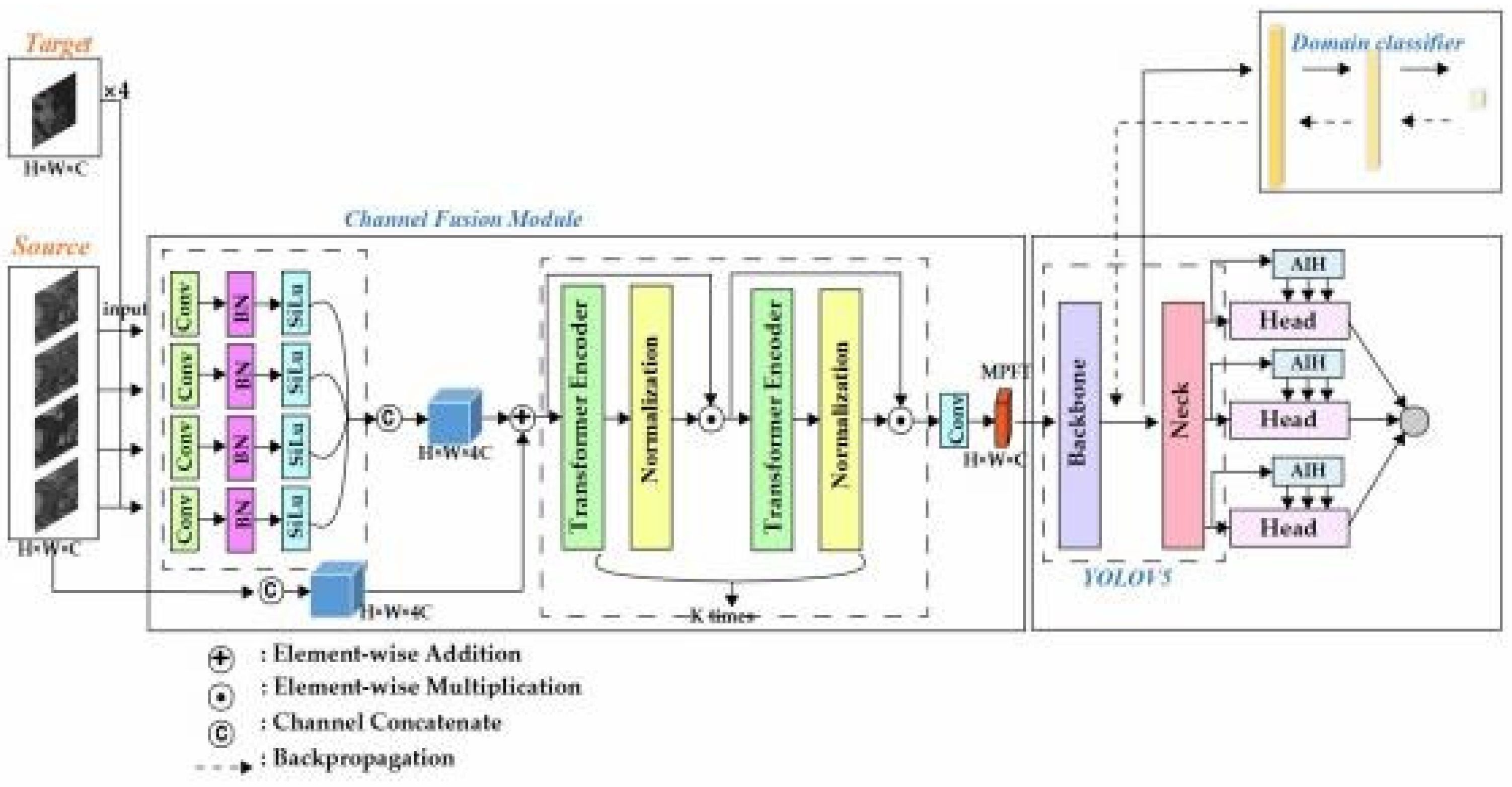
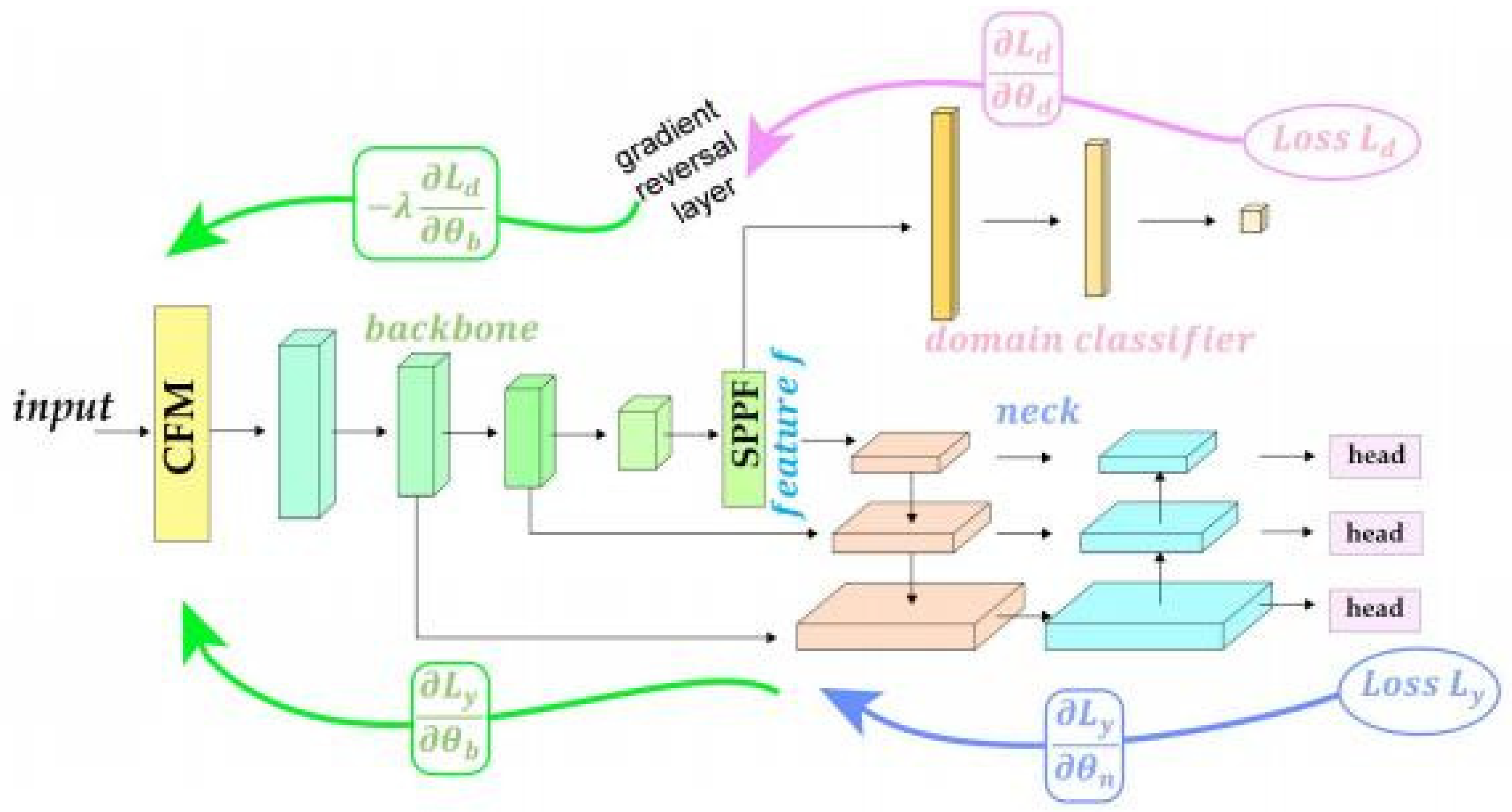
This paper proposes a complex background SAR ship target detection method based on fusion tensor and cross-domain adversarial learning, as illustrated in Figure 1. The model incorporates the CALM based on the YOLOV5s model, which achieves mutual adaptation between domains by inverting the gradient to bring the feature distribution distances between the source and target domains closer. Based on this approach, the proposed CFM extracts unique features from the fully polarised image and common features through convolutional neural network and Transformer respectively. This completes the fusion and feature extraction of the fully polarised image, significantly enriching the model’s feature information. The decoupling method forms AIH that separates the classifiers from the traditional detection head. This greatly alleviates the problem of susceptibility to complex background interference caused by the coupling of the detection head and reduces the occurrence of false positives.

All four polarised images are of size H×W×C. In the CFM the images from the four polarisations are input from the source, and their unique features are extracted separately. The features are then concatenated using ‘concatenate’ to form a fusion tensor of size H × W × 4C. Residuals are concatenated with the images that have not undergone feature extraction. The tensor obtained by concatenating the four polarisations is compressed into a tensor of size H × W × C by extracting their common features using a Transformer Encoder. This compressed tensor is referred to as the Multi-Polarisation Fusion Tensor (MPFT) in this paper. The MPFT contains both the unique features of the four polarisations and their common features, resulting in a high information content.

The training process involves combining YOLOV5s and CALM. The Backbone of YOLOV5 extracts features from the MPFTs generated from both the source and target domains. These features are then used for domain classification and feature fusion operations in the Neck part of YOLOV5. The resulting losses are the domain classification loss and target detection loss. It should be noted that in unsupervised training for the target domain, the feature extraction tensor specific to the target domain will not enter the Neck. This means that it will not calculate the target detection loss during training, but only the loss in domain classification.

The paper uses a fully polarised SAR image as the training set, as illustrated in Figure 2.

In the detection head section of YOLOV5, both the traditional YOLOV5 detection head and the AIH proposed in this paper calculate the loss simultaneously. The traditional detection head calculates the localisation loss, confidence loss, and category probability loss. In contrast, the AIH only calculates the category probability loss and replaces the final result of the traditional detection head. The experiments in this paper use a single polarised image as the target domain. To match the input of the multipolarised source domain, the target domain will be replicated four times as input.

3.2. Cross-Domain Adversarial Learning Module

SAR images are captured in complex and variable scenes, and image resources are often expensive and scarce. Directly using the training results of a dataset in a different scene with a different feature distribution often leads to unsatisfactory results.

Lyu et al. [27], proposed a scheme to effectively bring two different domain-distributed datasets closer together, achieving domain adaptation between real SAR datasets and simulated SAR images, and improving the cross-domain generalization ability of the detection model.

This paper proposes a cross-domain adversarial learning module, as shown in Figure 4. The module assumes datasets from two different domain distributions. When the source domain is a labelled dataset and the target domain is an unlabelled dataset, both with a certain distance between their domain distributions before the model is trained. The CALM trains a domain classifier to distinguish images from different domains by minimizing the domain classification loss. It then manipulates the gradient flow inversely by inverting the gradient to narrow the distance between the source and target domains. This achieves the effect of migration learning with high generalization ability.

Assume that the input sample x ∈ X, x is mapped by the CNN network and the output is y ∈ Y, where Y is the feature distribution space of the output result. the square and the circle in Figure 3. denote the feature distribution spaces S(x, y) and 丁(x, y) of the source and target domains, respectively, and there are multiple samples belonging to different categories within the space. In order to allow the source domain to accurately predict the target domain with its different distributions, the CALM needs to complete two tasks, the first task is to distinguish the different distributions within the source domain, i.e., the most basic YOLO target detection task, to minimise the target detection loss, so that the class boundary can be transformed from a random state before training to an accurate classification state after training. The second task is to close the distance between S(x, y) and 丁(x, y) so that the source and target domains have similar feature distributions. By this method, even if the target domain has no labels, it can be directly predicted efficiently. The specific process is described below.

Each input sample x has the label d ∈ {0,1} of the domain it belongs to, where the source domain is 0 the target domain is 1. In the experiments of this paper the input source domain is the fully polarised dataset with labels, which needs to be entered into the model after feature fusion. The target domain is the unipolarised dataset HRSID, trained without labels, which enters the model after from the polarisation fusion module. As shown in Figure 4. the whole mapping of the model is divided into three parts. The first part is the feature extraction module backbone, which goes from the head of the overall model to the end of the SPPF module of YOLOV5 to get the feature f, which is used by the feature extractor Gb to denote the parameters trained to θb. The second part is the YOLOV5’s feature fusion module, neck, which finally outputs the results of target detection, denoted by Gn, with the parameter θn. The third part is the domain classifier, which is used to learn the domain to which the sample x belongs, denoted by Gd and parameterised by θd. In addition, the target domain only goes through backbone and domain classifier during training, and all three modules of the source domain need to participate and calculate the corresponding loss.

The training process requires the features f to be discriminative, i.e., to be able to do the job of target detection correctly, i.e., the source domain needs to be trained in such a way that the YOLO target detection loss Ly is minimised. In addition, f needs to be domain invariant, i.e., it is necessary that the feature distribution S(x, y) of the source domain and the feature distribution 丁(x, y) of the target domain are as close as possible to each other and have a certain degree of similarity. The approach adopted is to use Gd to learn the domain to which the sample x belongs and Gb to bring the domain closer. That is, to minimise the loss on θd and maximise the loss on θb. And in order to maximise the loss on θf, a gradient reversal layer (GRL) operation is performed by multiplying a negative number to the gradient when the gradient of the domain classifier is backpropagated to the backbone. What the GRL does is, multiply the error passed to this layer by a negative number −λ, which causes the network before and after the GRL to have its training objectives opposite to each other to achieve the effect of confrontation.

3.2.1. Loss Function

For the CALM as a whole, the following loss functions should be considered. In the source domain:

Lsource (θb, θn, θd) = Σ Ly (Gn (Gb (xi; θb); θn), yi)	(1)
i=1...N
di = 0

For the target domain there is:

	(2)
di = 1
di = 1

where i denotes the ith training sample. Ly is the loss for YOLO target detection, only di = 0 when the source domain calculates this part of the loss. Ld is the loss for domain classification, where θd takes a negative value, the minus sign indicates that the opposite direction of the gradient is taken, and λ is the learning rate. Thus the overall loss of the whole model has:

L(θb, θn, θd) = Lsource (θb, θn, θd) + Ltarget(θb, θd)

(3)

where L(.) is the overall loss of the model.

For training purposes, the overall loss needs to be minimized with:

(4)

Among them, training the feature extraction parameter θb and the feature fusion parameter θn makes the loss of target detection minimised, thus ensuring the correctness of the target detection result. Training the domain classifier parameter θd allows the domain classification loss to be maximised, thus bringing the feature distribution space of the source and target domains closer together.

3.2.2. Model Optimisation

It is worth noting that instead of fixing the adaptation factor λ in order to suppress the noise signal of the domain classifier at an early stage of the training process, λ is gradually changed from 0 to 1 as the training proceeds, i.e:

(5)

where y is a hyperparameter with an initial value of 10. p is the current number of training rounds/total number of rounds, which changes from 0 to 1 as the training progresses. Thus, λ has an initial value of 0, which gradually changes to 1 as the training progresses to achieve the purpose of suppressing early noise in the domain classifier.

3.3. Channel Fusion Module

Fully polarised SAR typically produces images with four polarisation channels: HH, HV, VH and VV. This approach can provide more comprehensive scattering information of the observed target, which is beneficial for detecting ship targets. Even if the target domain image is single-polarised, such as full-polarised data in the training data, the correlation between the polarisation channels should be fully exploited to improve the feature extraction capability of the network. This paper presents the CFM, illustrated in Figure 1.

Multimodal fusion can be performed at three levels: decision, feature, and pixel. However, pixel-level fusion is not recommended due to the high computational cost. To extract both local features under unipolarisation and global features under full polarisation simultaneously, this paper employs feature-level fusion.

The process involves first extracting the unique features under single polarisation using the basic Conv+BN+SiLu structure. Furthermore, to maintain the feature tensor size after extraction, it is crucial to regulate the convolution output tensor size by adjusting the convolution step size and padding.

(6)

where ΦHH, ΦVV, ΦHV, ΦVH represent the input HH,HV,VH,VV feature maps respectively. CBS(.) represents the Conv+BN+SiLu operation. ${\mathsf{\Phi }}_{\mathrm{V}\mathrm{V}}^{\mathrm{C} }$, ${\mathsf{\Phi }}_{\mathrm{V}\mathrm{V}}^{\mathrm{C} }$, ${\mathsf{\Phi }}_{\mathrm{H}\mathrm{V}}^{\mathrm{C} }$, ${\mathsf{\Phi }}_{\mathrm{V}\mathrm{H}}^{\mathrm{C} }$ represents the quadrupolarised feature tensor after CBS(.) extraction.

The feature extraction of the four polarised images before fusion is a feature-level fusion, which is conducive to the subsequent feature extraction of the fused tensor. Compared with the pixel-level fusion that directly splices the input images of the four polarisations, this method effectively saves computation and distinguishes the differences between different polarisations more obviously, which greatly enriches the semantic information of the fused tensor. The feature fusion process is described as:

(7)

where ⊕ stands for element-wise addition. H0 is the result after feature fusion.

After obtaining the feature fusion tensor H0 it is necessary to perform the extraction of fully polarised shared features, using transformer to perform this operation [34,35]. Transformer can learn remote dependency relationships of feature maps relative to CNN, because the calculation of self-attention is independent of the distance between pixels. The feature tensor H0 is put through k transformers with residual concatenation. Describe the process as:

Hi = Hi−1⨀N(丁(Hi))

(8)

where N (.) denotes the normalisation operation. 丁 (.) represents transformer operation. ⨀ stands for element-wise multiplication. Hi denotes the result after the ith transformer operation.

3.4. Anti-Interference Head

The interference from the complex background of SAR images often leads to False Positive detection results. This is particularly problematic as coastal facilities share similar features with target ships. To address this issue, this paper proposes the AIH model inspired by the decoupling head of YOLOVX [36,37]. The model aims to better isolate the target from the complex and variable background and reduce its influence on target detection.

In YOLOVX, the authors note that the classification and localisation tasks of the model have significant differences. They argue that the traditional coupling head can negatively impact the final detection results. To address this issue, the paper proposes splitting the original detection head into three separate heads. These heads predict the target’s category, localisation, and confidence, respectively. The authors claim that this approach leads to better generalization ability in both classification and localisation. This paper argues that decoupling the classification head from the traditional coupling head can improve the model’s ability to classify different categories. Additionally, decoupling is useful for distinguishing between the target and background information in YOLO, which can effectively improve the ability to reduce background interference. In practical applications of SAR ships, the model’s detection results are not substantially affected by the confidence level. Therefore, it is unnecessary to separate the confidence level into individual detection heads. Only the Classification head needs to be stripped out of the original detection head. To cope with the interference of the complex background, the AIH illustrated in Figure 5 is obtained. The process is as follows:

YOLOV5 has three sizes of detection heads, H×W×(156,512,1024), which predict large, medium and small targets, respectively. For a single detection head, the traditional YOLO algorithm compresses it into a tensor of size H×W×((4+1+C)×anchor) by one layer of convolution for the final decoding work, where 4 stands for the coordinates of the centre point (X,Y) and the length and width of the detection frames (w,h), 1 stands for the confidence level, C stands for the predicted number of categories, and anchor stands for the initial number of detection boxes in a grid cell

In this paper, a classification head of size H×W×(C×anchor) is peeled off by three-layer convolution in the traditional coupling head, and by decoding this tensor, the probability of the classification condition category of a certain detecting frame is obtained C1, C2, . . Cn , and therefore the probability of the detecting frame being background is 1 − C1 + C2 . . . + Cn . According to the above discussion, the result has a strong ability to distinguish between background and target. On the other hand, a positioning and confidence head of size H × W × 5 is obtained by one layer of convolution for calculating the positioning coordinates and confidence. Finally the results of the two detection heads are combined to get the prediction of the model.

During the training process, a large amount of SAR image data is used, and through repeated iterative training, the model is made to gradually learn the feature representations that effectively distinguish the target from the background. Eventually, the AIH is able to accurately distinguish the target ship from the coastal facilities in the target detection task with a low false alarm rate.

4. Experiments

In this part, specific experiments are carried out on the scheme proposed above. The main purpose of the experiments in this paper is to demonstrate that CALM has some cross-domain generalization capability, and that CFM and AIH can effectively improve the cross-domain generalization capability of the model. In this paper, the independently constructed SAR Full Polarisation Dataset (SFPD) is used as the source domain, and the HRSID dataset is used as the target domain. In addition, in order to ensure real-time target detection, the target domains involved in the training are not used for the evaluation of the model.

In the experiments, firstly, their cross-domain generalization ability will be tested under several current commonly used models, and after finding certain patterns, they will be improved by deep domain adaptation, and finally, some images of the training results of the models will be shown.

In this paper, the models are trained and evaluated on the Windows platform, and the GPU used is NVIDA RTX-3090.

4.1. Model Evaluation Methodology

The model evaluation metrics in this paper are and F1 and AP (Average Precision). Before calculation firstly the confusion matrix of the trained model under the test set needs to be calculated. If the intersection and integration ratio (IOU) of the detected frame to the true frame is greater than 0.5, the detection is considered to be correct and is True Positive (TP). If the background is wrongly predicted as the target it is False Positive(FP) and if the target is missed, it is False Negative(FN). Thus, the model’s accuracy Formula (9) is obtained, and the accuracy indicates the proportion of correctly positive predictions of the model to the proportion of all positive predictions.

(9)

The recall of the model represents the proportion of correct predictions that are positive to the proportion of all that are actually positive, and is given by Formula (10):

(10)

After getting precision and recall, there are two metrics to evaluate the model. However, usually the two hold each other back, so it is necessary to combine the two to be the final evaluation metrics, so there are F1 and AP as the final evaluation metrics.

F1 is calculated as Formula (11):

(11)

Whereas the process of calculating AP is more complex, in YOLO, the process of calculating AP is as follows:

• For each category, first sort all the prediction frames according to the confidence level from high to low.
• For each prediction box, calculate its IoU (Intersection over Union) value with all the real boxes in the same category, and find the real box with the largest IoU value.
• If the IoU value is greater than a set threshold (usually 0.50), the prediction box is considered as a correct prediction, otherwise it is considered as an incorrect prediction.
• For each confidence threshold, calculate the Precision and Recall at that threshold. In a nutshell, the process of AP calculation is to determine whether the prediction frame is correct or not by comparing the IoU values between the prediction frame and the real frame, and then calculate the precision and recall based on different confidence thresholds, and finally plot the PR curve and calculate the AP.

4.2.1. HRSID

The HRSID dataset [38], which was released in January 2020, is a high-resolution SAR image dataset primarily used for ship detection, semantic segmentation, and instance segmentation tasks. The dataset comprises 5,604,800 ship images captured by Sentinel-1B, TerraSAR-X, and TanDEM-X satellites. The imaging area was selected in ports with high cargo handling capacity or busy canals crisscrossing the trading city. The images were captured using StripMap imaging mode with a resolution of better than 3m and polarisation modes of HH, HV, and VV. The scanning range is 270km. The dataset comprises 5604 high-resolution SAR images, each with a resolution of 800*800 pixels, and 16951 ship instances. Figure 6 displays the specific images.

This paper uses HRSID as the target domain for model training and evaluation. HRSID was chosen due to its significant number of images and its high-resolution SAR image dataset with the same target as SFPD.

4.2.2. SAR Full Polarization Dataset

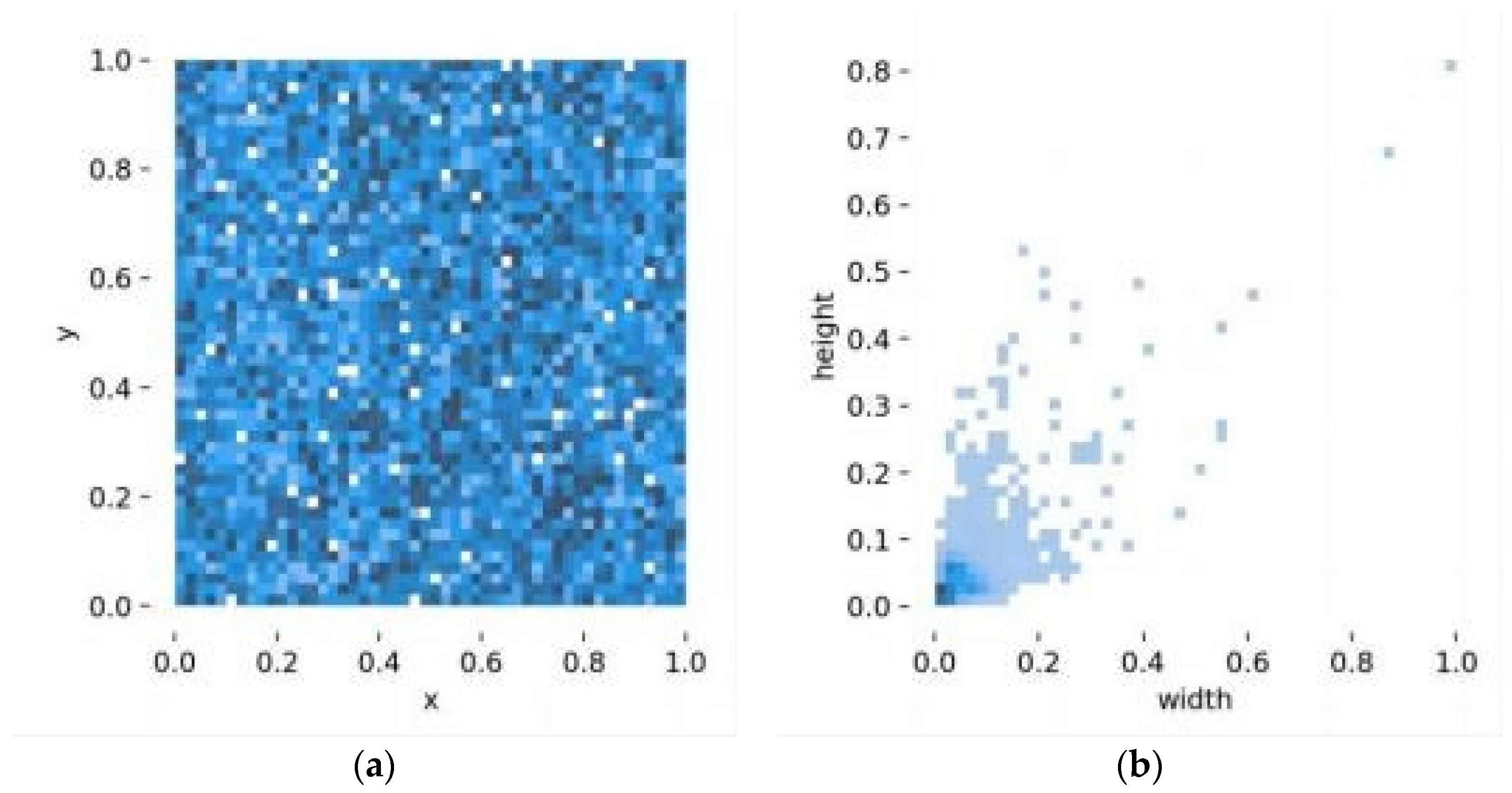
The dataset captured harbour and maritime targets using on-board SAR with 8m resolution and QPSI as the imaging mode. Full polarisation was employed, resulting in 4668 images, each measuring 416*416 pixels. In total, 15,212 targets were identified, with an average pixel value of 412.53. Figure 8 displays some of the images. Figure 7(a) shows the heat map of the positional distribution of the images, indicating a more uniform distribution of colour blocks and therefore a more uniform distribution of target frames. Figure 7(b) displays the heat map of the aspect distribution of the target box, revealing a concentration of dark colour blocks in the lower left corner of the image, indicating a higher number of small targets.

4.3. Multi-Model Comparative Experiments

The experiments in this paper begin by exploring the target detection capability of cross-domain generalization on several currently dominant models. Usually, the learning ability of the models is improved with the deepening of the network.

However, the experiments in this paper find that, as shown in Table 1, the learning ability of the YOLOV5 model in terms of cross-domain generalization detection decreases with the depth of the model under the same structure. In YOLOV5, compared to the s model, the m model decreases Precision by 4.4%, Recall by 1.2%, AP by 2.1%, F1 by 2.4%.Compared to the m model, the l model decreases Precison by 1.6%, Recall by 0.4%, AP by 1.9%, F1 by 0.8%. In this paper, we argue that this decrease is inevitable, although models with larger parameters learn more semantic features from the source domain, resulting in a higher generalization ability on the source domain. However, this high generalization ability to the target domain is likely to become overfitting. As for the two-stage large model like Faster-RCNN, the AP is only 18.7%, which basically does not have the ability of cross-domain generalised detection. Moreover, Azizpour et al. [39], pointed out that performance can be improved by increasing the width and depth of the network when the source and target domains are close. However, excessive parameterization may damage feature information, causing the learned ability to deviate from the target domain. Therefore, in transfer learning, caution should be exercised in selecting models and datasets to avoid the negative impact of increasing parameter count.

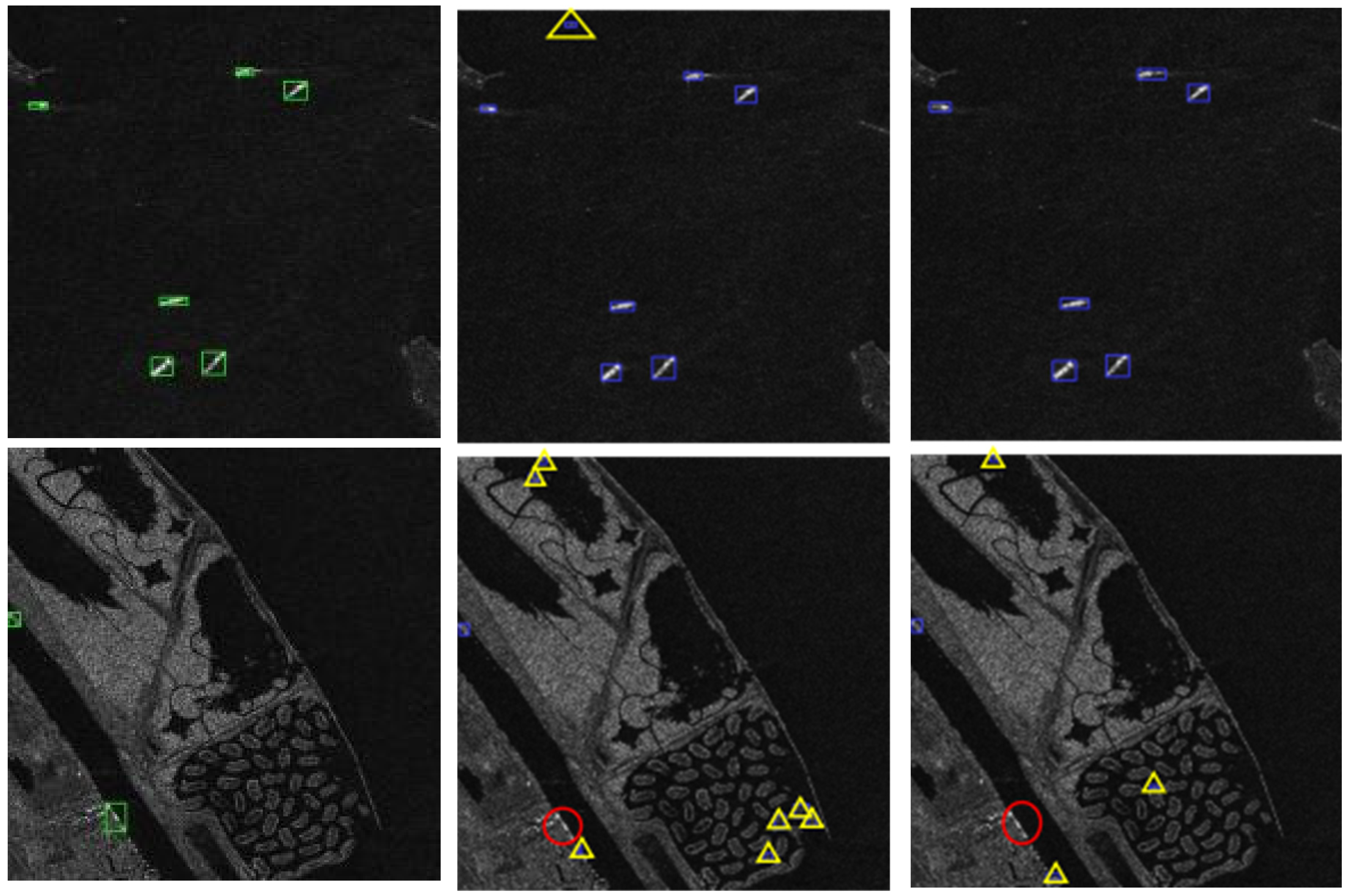
The detection images of various models are shown in Figure 9, where the green box is Ground Truth, the blue box is the model detection result, the red ellipse is False Nagative, and the yellow triangle is False Positive. it can be seen that the models with a larger number of parameters are more likely to be False Positive due to overfitting. And although Faster-RCNN can successfully detect some targets, too much False Positive has made it lose its usability.

Figure 9. Plot of the results of the multi-model comparison experiment.

Figure 9. Plot of the results of the multi-model comparison experiment.

4.4. Model Improvement Results

This paper proposes a complex background SAR ship target detection method based on fusion tensor and cross-domain adversarial learning. The aim is to solve the problem of low cross-domain generalised detection capability of traditional models. The proposed fusion of CALM and YOLOV5s transforms the model into a cross-domain model. The CFM and AIH models are fused sequentially to enhance the model’s target detection ability in the cross-domain generalization problem. It should be noted that, unlike traditional ablation experiments, this paper does not separately validate the effects of CFM+AIH. This is because the CFM and AIH models are two models designed based on the CALM cross-domain model to take full advantage of the correlation between the fully polarised image data and to improve the model’s ability to resist the interference of complex backgrounds. The final model improves Precision by 2.3%, Recall by 5.2%, AP by 4.1%, and F1 by 4.2% compared to the baseline model based on YOLOV5s. The specific experimental results are shown in Table 2. Compared with YOLOV8s, which is the best performing model among all models, Precision is improved by 4.9%, Recall is improved by 3.3%, AP is improved by 2.4%, and F1 is improved by 3.9%.

4.4.1. Analysis of CALM Results

After implementing the CALM structure, Precision increased by 0.5%, Recall improved by 1.8%, AP improved by 2.8%, and F1 improved by 1.4%. All parameters have been improved, but the improvement in precision is not very significant. This is because CALM forces the source and target domains to be closer together, causing the target domain to learn features belonging to the source domain that interfere with its own detection, resulting in little improvement in reducing false positives. However, in practical applications, the primary objective is to detect the target as quickly as possible after a single detection. Therefore, this paper argues that the Recall metric is more crucial in the real-time detection of SAR images. The CFM and AIH proposed in this paper will significantly improve Precision and further enhance Recall. The specific experiments are described in detail below.

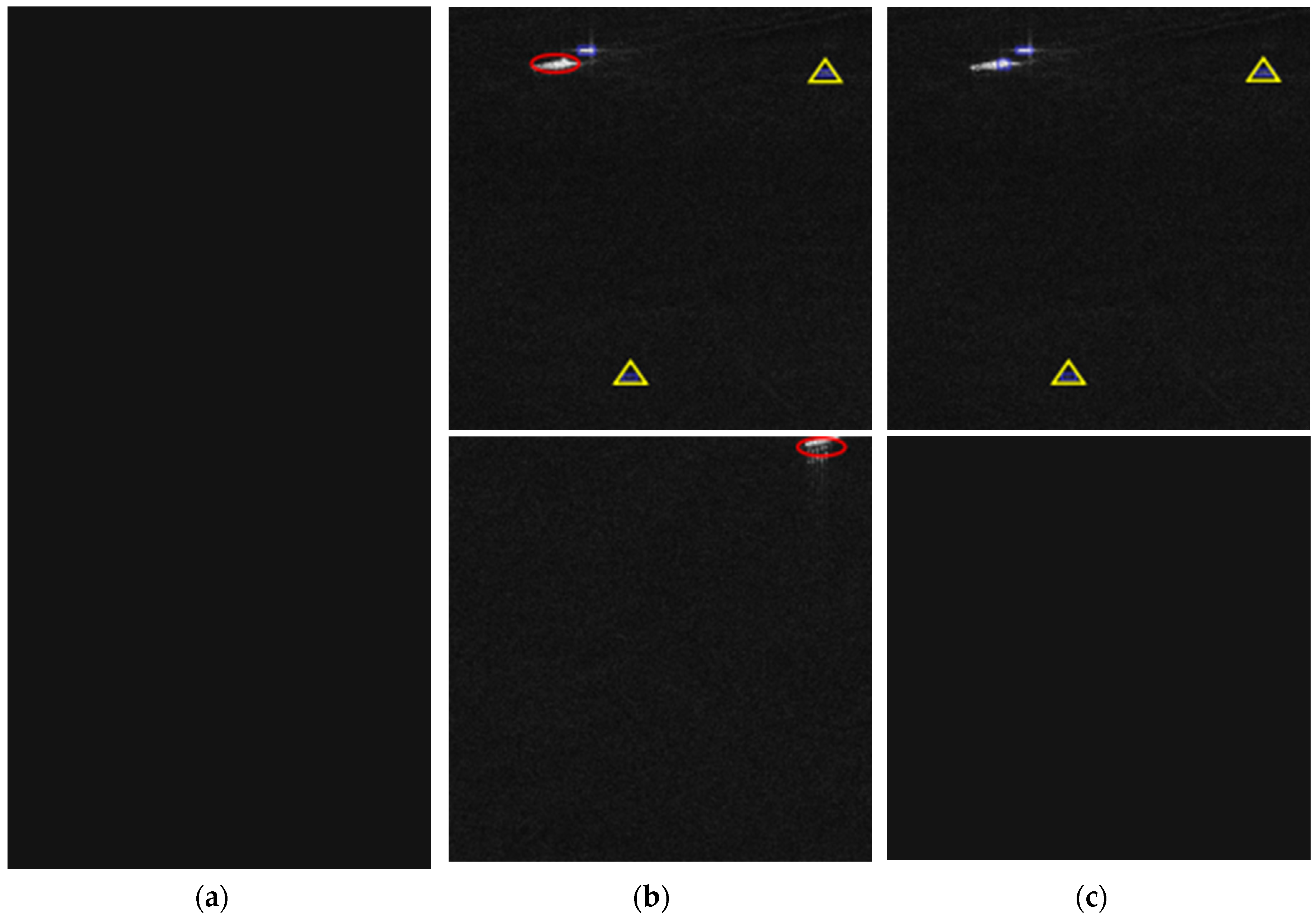
Figure 10 shows the detection picture of the CALM experiment. It is evident that the addition of CALM significantly reduces the False Negative phenomenon of the model. However, there is no significant improvement in the False Positive phenomenon. To address this issue, this paper proposes the design of two modules, CFM and AIH.

Figure 10. CALM experiment results: (a) Ground Truth image; (b) baseline model detection image. (c) YOLOV5+CALM detection image.

Figure 10. CALM experiment results: (a) Ground Truth image; (b) baseline model detection image. (c) YOLOV5+CALM detection image.

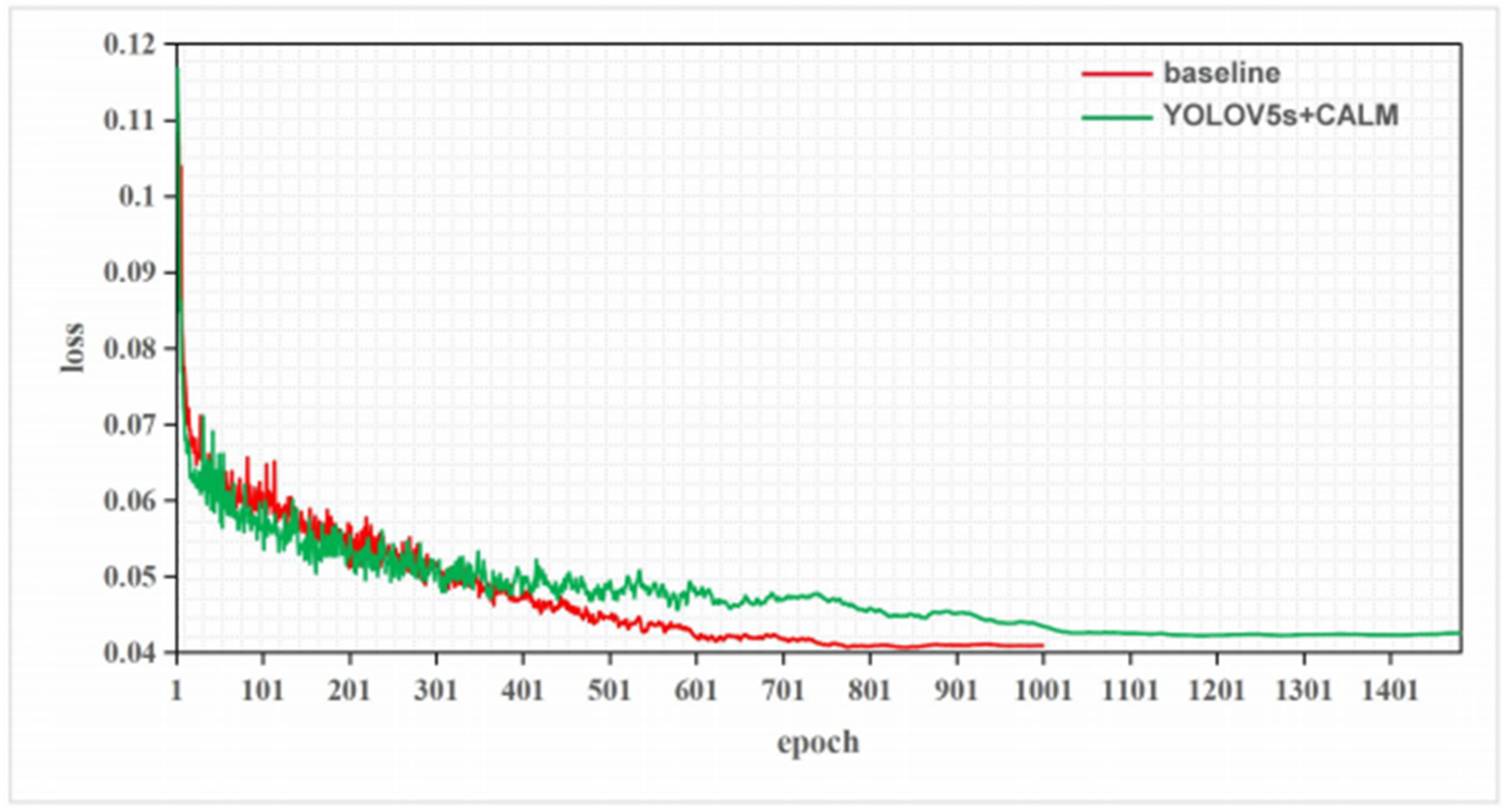
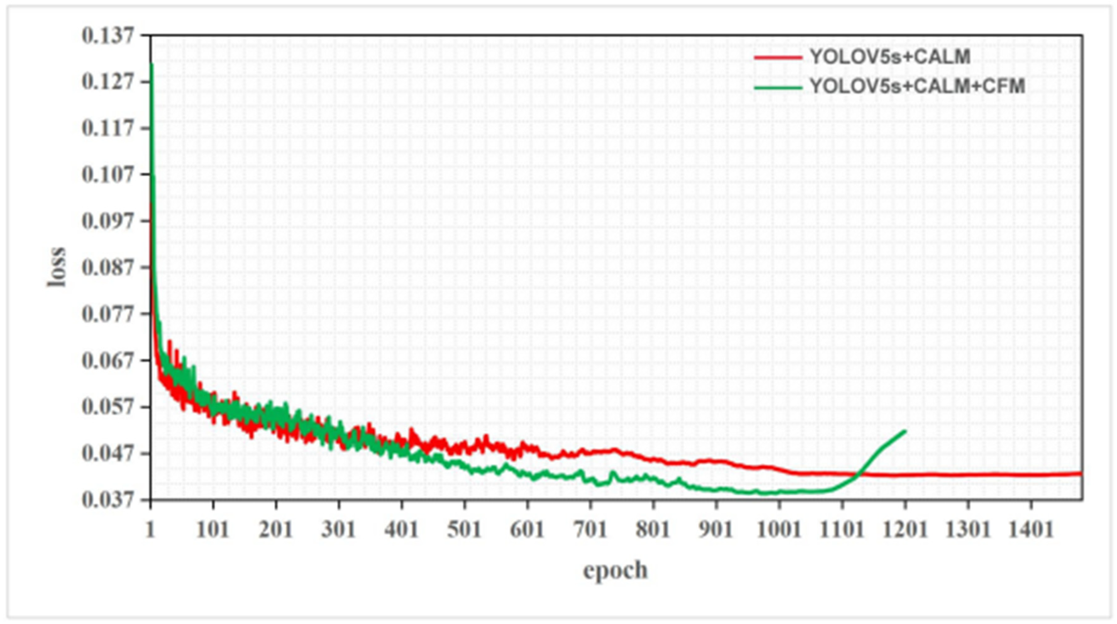
Figure 11 shows a line graph that illustrates the loss in the source domain over epochs. The YOLOV5+ATL model converges slower and has a higher loss compared to the baseline. The interference of the source domain in the calculation of the target detection loss is believed to be caused by the fact that the source and target domains enter the feature extraction module simultaneously. It is important to note that this is a subjective evaluation and should be clearly marked as such. This interference does not directly affect the detection of the target domain. However, it reduces the target detection ability learned by the model, which indirectly affects the detection of the target domain.

Figure 11. Line graph of the change in loss for the CALM experimental validation set.

Figure 11. Line graph of the change in loss for the CALM experimental validation set.

This paper argues that the phenomenon can be mitigated by separating the feature extraction module of the source and target domains. This requires further experimental investigation.

4.4.2. Analysis of CFM Results

The model that incorporates the designed CFM module improves Precision by 0.1%, Recall by 2%, and F1 by 1.3%. The experiments demonstrate that CFM effectively fuses the features of the four polarisations and fully utilises them to enrich the semantic features of the model, thereby further improving its cross-domain generalization ability.

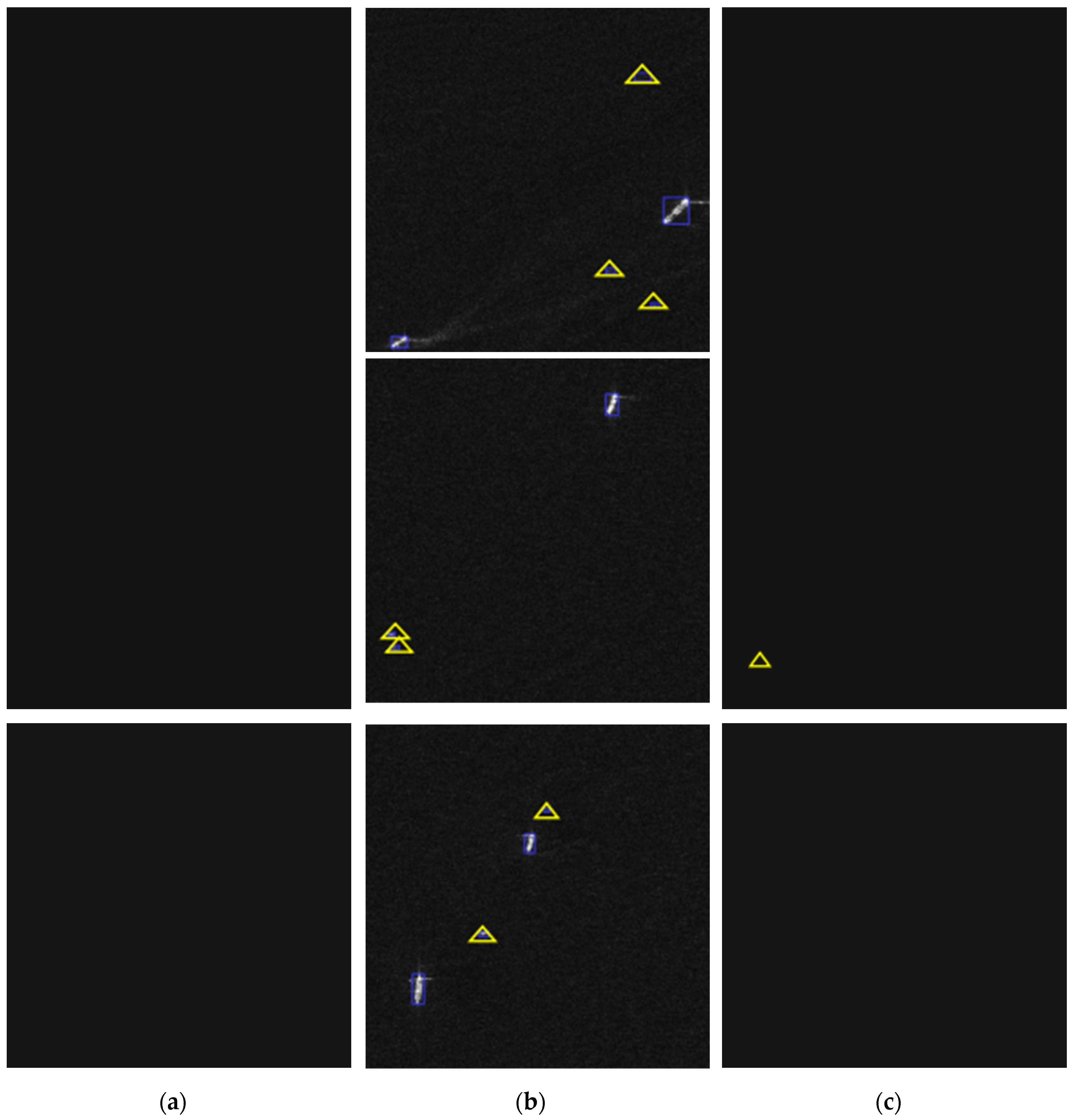
Figure 12 shows the detection image after adding CFM. The experiment found that the model’s False Positive phenomenon was reduced after adding CFM.

Figure 12. CFM experiment results: (a) Ground Truth image; (b) YOLOV5+CALM detection image;. (c) YOLOV5+CALM+CFM detection image.

Figure 12. CFM experiment results: (a) Ground Truth image; (b) YOLOV5+CALM detection image;. (c) YOLOV5+CALM+CFM detection image.

Figure 13 shows a line graph of the loss on the validation set during the CFM experiments as a function of the training batch. It can be observed that the convergence speed improved after adding CFM, resulting in lower loss after final convergence. However, after 1000 rounds, the loss gradually starts to increase, indicating network degradation. In this paper, we suggest that the reason for overfitting on the target domain is due to the extraction of too many features from the source domain using CFM. However, CFM does have an enhancement effect, and overfitting can be effectively controlled by appropriately limiting the number of training epochs. The subsequent experiments showed that the inclusion of the designed AIH module effectively reduced the occurrence of network degradation.

Figure 13. Line graph of the change in loss for the CFM experimental validation set.

Figure 13. Line graph of the change in loss for the CFM experimental validation set.

It is worth noting that CFM not only improves the cross-domain model proposed in this paper, but also shows remarkable capability even when used alone on traditional non-cross-domain models. In this paper, the CFM module is trained and evaluated simultaneously on the SFPD dataset for the CFM module, and the results are obtained as shown in Table 3. It can be found that compared to the model under single polarisation, the polarisation fusion with CFM improves Precision by 1.5%, Recall by 9.6%, AP by 5.2%, F1 by 5.9%, while Params and GFlops only increase by 1.37 and 0.8, respectively, thus highlighting the importance of utilising multi-polarised data.

4.4.3. Analysis of AIH Results

The addition of the designed AIH module to CALM+CFM resulted in a 1.7% improvement in Precision, 1.4% improvement in Recall, 2.3% improvement in AP, and 1.5% improvement in F1. It was found that the Recall of the model continued to improve and there was a further breakthrough in Precision after the addition of the AIH module. This indicates that AIH has a strong ability to resist background interference, which can effectively distinguish the complex background from the target to be detected and mitigate the False Positive phenomenon.

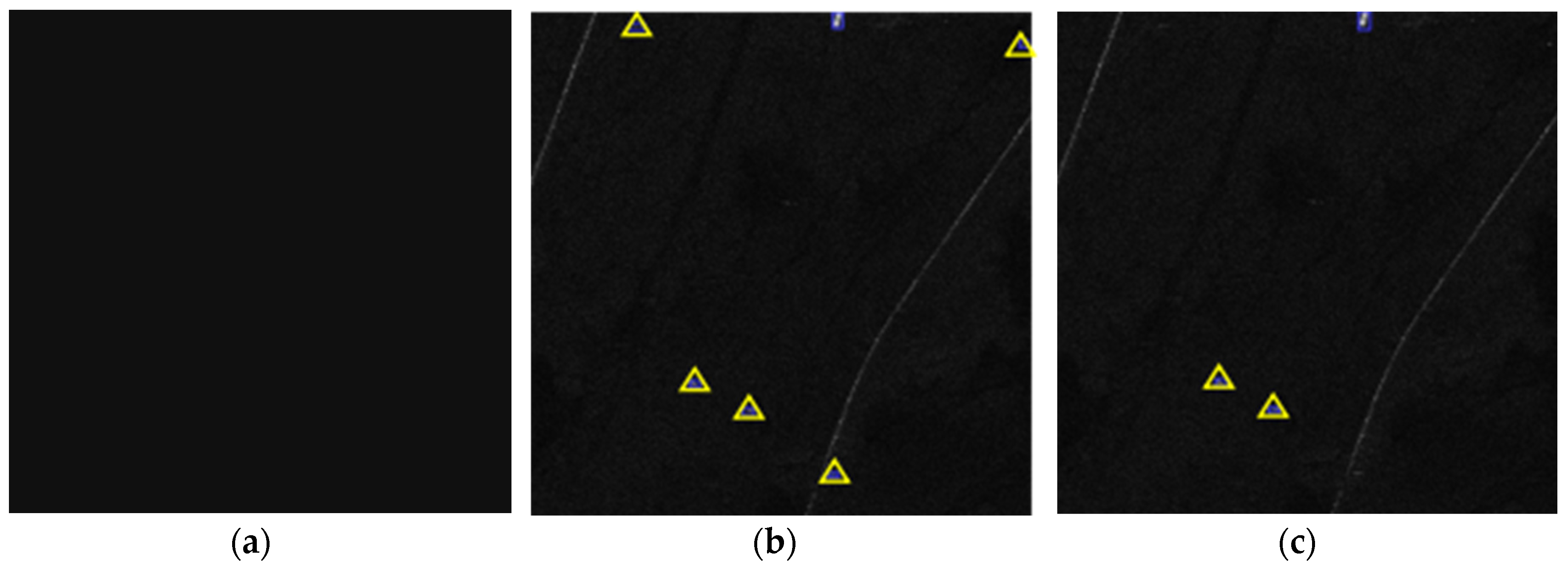
The detection image after adding AIH is shown in Figure 14. It is found that the False Positive phenomenon of the model after adding the AIH is decreased very significantly. The figure’s original target was misjudged due to interference from the complex background, which resembled the light spots of the ship target. However, the AIH module’s fusion eliminated many of these falsely detected target frames.

Figure 14. AIH experiment results: (a) Ground Truth image; (b) YOLOV5+CALM+CFM detection image; (c) YOLOV5+CALM+CFM+AIH detection image.

Figure 14. AIH experiment results: (a) Ground Truth image; (b) YOLOV5+CALM+CFM detection image; (c) YOLOV5+CALM+CFM+AIH detection image.

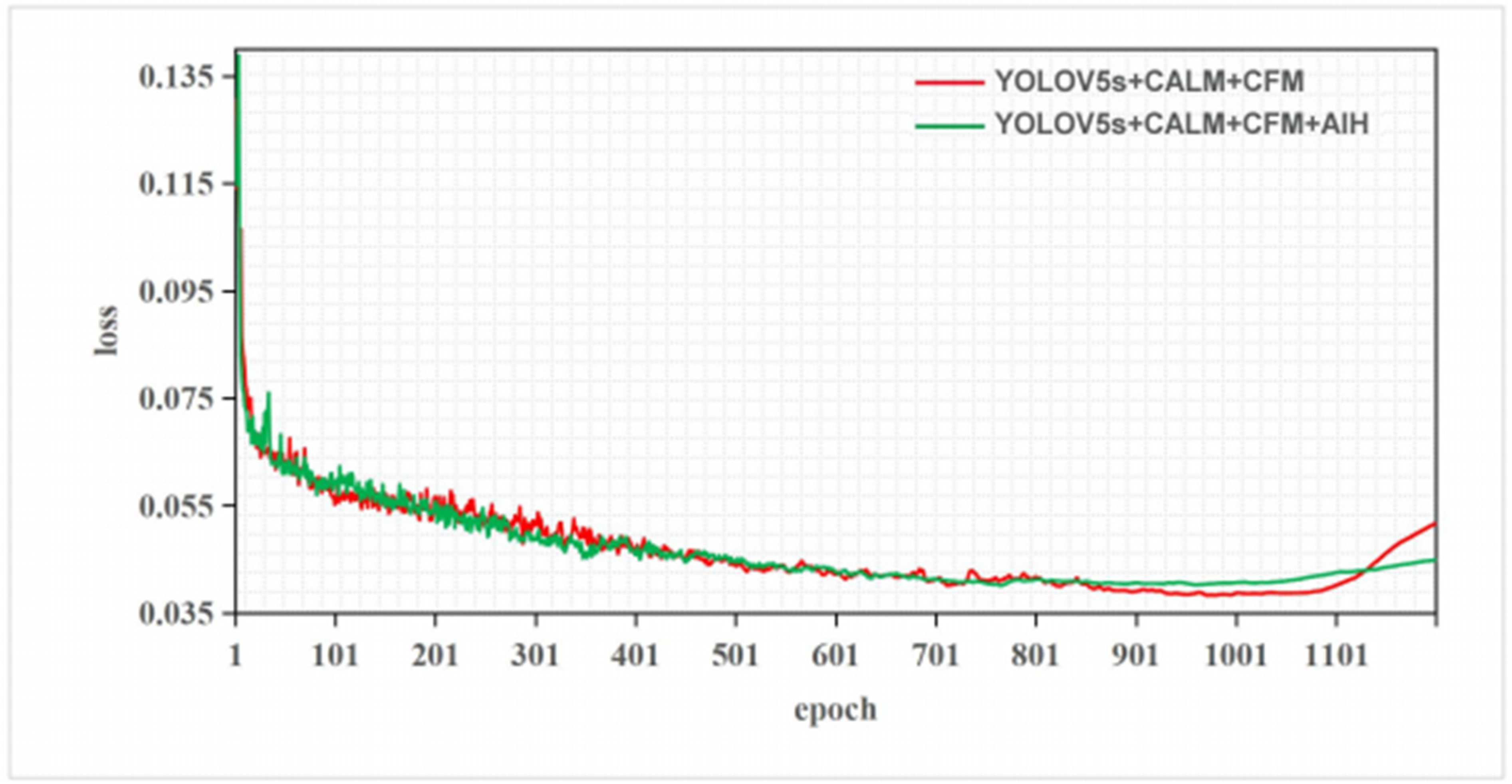
Figure 15 shows a line graph of the loss on the validation set during the AIH experiments as the training batch changes. It can be observed that the magnitude of the loss becomes less jittery after adding AIH, and the network degradation phenomenon is alleviated to some extent. This is because the decoupling method of AIH effectively separates the classification task from the localization task, allowing for more stable model training.

Figure 15. Line graph of the change in loss for the AIH experimental validation set.

Figure 15. Line graph of the change in loss for the AIH experimental validation set.

5. Discussion

This paper proposes a complex background SAR ship target detection method based on fusion tensor and cross-domain adversarial learning. Three modules, CALM, CFM, and AIH, are designed to improve the cross-domain generalised detection capability of current target detection models. The model makes full use of the rich feature information of the omnipolar dataset and alleviates the problems of missing target features and susceptibility to interference by complex backgrounds due to the coupling of detection models. Compared to the best-performing YOLOV8s model among typical mainstream models, this model improves Precision by 4.9%, Recall by 3.3%, AP by 2.4%, and F1 by 3.9%.

The experiments in this paper show that deeper models are prone to reduced cross-domain generalization detection ability, which is considered to be caused by overfitting.

In the CALM experiment, the recall was significantly improved, but the change in precision was not very noticeable. The experiments in this paper suggest that this may be due to differences in the distribution between the source and target domains. Domain adaptation causes the target domain to learn a feature distribution that does not belong to itself, which can affect the final detection results. Future experiments will further investigate cross-domain migration learning of SAR images to address the aforementioned issues.

References

- Yu, W.; Li, J.; Wang, Z.; Yu, Z. Boosting SAR Aircraft Detection Performance with Multi-Stage Domain Adaptation Training. Remote Sens. 2023, 15, 4614. [Google Scholar] [CrossRef]
- Zhang, X.; Hu, D.; Li, S.; Luo, Y.; Li, J.; Zhang, C. Aircraft Detection from Low SCNR SAR Imagery Using Coherent Scattering Enhancement and Fused Attention Pyramid. Remote Sens. 2023, 15, 4480. [Google Scholar] [CrossRef]
- Lan, Z.; Liu, Y.; He, J.; Hu, X. PolSAR Image Classification by Introducing POA and HA Variances. Remote Sens. 2023, 15, 4464. [Google Scholar] [CrossRef]
- Weiss, M. Analysis of some modified cell-averaging CFAR processors in multiple-target situations. IEEE Trans. Aerosp. Electron. Syst. 1982, 18, 102–114. [Google Scholar] [CrossRef]
- Liu, T.; Yang, Z.; Yang, J.; Gao, G. CFAR Ship Detection Methods Using Compact Polarimetric SAR in a K-Wishart Distribution. IEEE J. Sel. Top. Appl. Earth Obs. Remote Sens. 2019, 12, 3737–3745. [Google Scholar] [CrossRef]
- Li, T.; Peng, D.; Chen, Z.; Guo, B. Superpixel-level CFAR detector based on truncated gamma distribution for SAR images. IEEE Geosci. Remote Sens. Lett. 2020, 18, 1421–1425. [Google Scholar] [CrossRef]
- Krizhevsky, A.; Sutskever, I.; Hinton, G. ImageNet Classification with Deep Convolutional Neural Networks. Communications of the ACM 60 (2012); pp. 84-90.
- He, K.; Zhang, X.; Ren, S.; Sun, J. Deep Residual Learning for Image Recognition. In Proceedings of the 2016 IEEE Conference on Computer Vision and Pattern Recognition (CVPR), Las Vegas, NV, USA; 2016; pp. 770–778. [Google Scholar]
- Huang, G.; Liu, Z.; Van Der Maaten, L.; Weinberger, K.Q. Densely Connected Convolutional Networks. In Proceedings of the 2017 IEEE Conference on Computer Vision and Pattern Recognition (CVPR), Honolulu, HI, USA; 2017; pp. 2261–2269. [Google Scholar]
- Wang, C.; Liao, M.; Wu, Y.; Chen, P.; Hsieh, J.; Yeh, I. CSPNet: A New Backbone that can Enhance Learning Capability of CNN. In Proceedings of the 2020 IEEE/CVF Conference on Computer Vision and Pattern Recognition Workshops (CVPRW), Seattle, WA, USA; 2020; pp. 1571–1580. [Google Scholar]
- Girshick, R.; Donahue, J.; Darrell, T.; Malik, J. Rich Feature Hierarchies for Accurate Object Detection and Semantic Segmentation. In Proceedings of the 2014 IEEE Conference on Computer Vision and Pattern Recognition (CVPR), Columbus, OH, USA, 23–28 June 2014; pp. 580–587. [Google Scholar]
- Girshick, R. Fast R-CNN. In Proceedings of the 2015 IEEE International Conference on Computer Vision (ICCV). 2015; pp. 1440-1448.
- Ren, S.; He, K.; Girshick, R.; Sun, J. Faster R-CNN: Towards Real-Time Object Detection with Region Proposal Networks. IEEE Transactions on Pattern Analysis and Machine Intelligence. June 2016; pp. 1137-1149.
- Redmon, J.; Divvala, S.; Girshick, R.; Farhadi, A. You Only Look Once: Unified, Real-Time Object Detection. In Proceedings of the 2016 IEEE Conference on Computer Vision and Pattern Recognition (CVPR), Las Vegas, NV, USA; 2016; pp. 779–788. [Google Scholar]
- Redmon, J.; Farhadi, A. YOLO9000: Better, Faster, Stronger. In Proceedings of the 2017 IEEE Conference on Computer Vision and Pattern Recognition (CVPR), Honolulu, HI, USA; 2017; pp. 6517–6525. [Google Scholar]
- Redmon, J.; Farhadi, A. YOLOv3: An Incremental Improvement. Apr 2018.
- Liu, W.; Anguelov, D.; Erhan, D.; Szegedy, C.; Reed, S.; Fu, C.Y.; Berg, A.C. SSD: Single Shot MultiBox Detector. In European Coference on Computer Vision; Lecture Notes in Computer Science; Springer: Cham, Switzerland, 2016; pp. 21–37. [Google Scholar]
- Lin, T.; Goyal, P.; Girshick, R.; He, K.; Dollár, P. Focal Loss for Dense Object Detection. In Proceedings of the 2017 IEEE International Conference on Computer Vision (ICCV), Venice, Italy; 2017; pp. 2999–3007. [Google Scholar]
- Lin, T.; Dollár, P.; Girshick, R.; He, K.; Hariharan, B.; Belongie, S. Feature Pyramid Networks for Object Detection. In Proceedings of the 2017 IEEE Conference on Computer Vision and Pattern Recognition (CVPR), Honolulu, HI, USA, 2017. pp. 936–944.
- Li, H.; Xiong, P.; An, J.; Wang, L. Pyramid Attention Network for Semantic Segmentation. arXiv 2018, arXiv:1805.10180. [Google Scholar]
- Guo, Y.; Zhou, L. MEA-Net: A Lightweight SAR Ship Detection Model for Imbalanced Datasets. Remote Sens. 2022, 14, 4438. [Google Scholar] [CrossRef]
- Zhou, Y.; Liu, H.; Ma, F.; Pan, Z.; Zhang, F. A Sidelobe-Aware Small Ship Detection Network for Synthetic Aperture Radar Imagery. IEEE Transactions on Geoscience and Remote Sensing, 2024; pp. 1-16.
- Tang, G.; Zhao, H.; Claramunt, C.; Zhu, W.; Wang, S.; Wang, Y.; Ding, Y. PPA-Net: Pyramid Pooling Attention Network for Multi-Scale Ship Detection in SAR Images. Remote Sens. 2023, 15, 2855. [Google Scholar] [CrossRef]
- Hu, J.; Zhi, X.; Shi, T.; Zhang, W.; Cui, Y.; Zhao, S. PAG-YOLO: A Portable Attention-Guided YOLO Network for Small Ship Detection. Remote Sens. 2021, 13, 3059. [Google Scholar] [CrossRef]
- Huang, Z.; Pan, Z.; Lei, B. What, Where, and How to Transfer in SAR Target Recognition Based on Deep CNNs. IEEE Transactions on Geoscience and Remote Sensing, 2020; pp.2324-2236.
- Tang, X.; Sun, Y.; Liu, S.; Yang, Y. DETR with Additional Global Aggregation for Cross-domain Weakly Supervised Object Detection. In Proceedings of the 2023 IEEE/CVF Conference on Computer Vision and Pattern Recognition (CVPR), Vancouver, BC, Canada; 2023; pp. 11422–11432. [Google Scholar]
- LYU, X.; Qiu, X.; Yu, W.; XU, F. Simulation-assisted SAR target classification based on unsupervised domain adaptation and model interpretability analysis, Journal of Radars, 2022, 11(1); pp. 168-182.
- Ma, Y.; Yang, Z.; Huang, Q.; Zhang, Z. Improving the Transferability of Deep Learning Models for Crop Yield Prediction: A Partial Domain Adaptation Approach. Remote Sens. 2023, 15, 4562. [Google Scholar] [CrossRef]
- Xu, X.; Zhang, X.; Shao, Z.; Shi, J.; Wei, S.; Zhang, T.; Zeng, T. A Group-Wise Feature Enhancement-and-Fusion Network with Dual-Polarization Feature Enrichment for SAR Ship Detection. Remote Sens. 2022, 14, 5276. [Google Scholar] [CrossRef]
- Zhao, Z.; Bai, H.; Zhang, J.; Zhang, Y.; Xu, S.; Lin, Z.; Timofte, R.; Gool, L.V. CDDFuse: Correlation-Driven Dual-Branch Feature Decomposition for Multi-Modality Image Fusion. 2023 IEEE/CVF Conference on Computer Vision and Pattern Recognition (CVPR), Vancouver, BC, Canada, 2023; pp. 5906-5916.
- Xu, Z.; Zhai, J.; Huang, K.; Liu, K. DSF-Net: A Dual Feature Shuffle Guided Multi-Field Fusion Network for SAR Small Ship Target Detection. Remote Sens. 2023, 15, 4546. [Google Scholar] [CrossRef]
- Zhang, J.; Lei, J.; Xie, W.; Fang, Z.; Li, Y.; Du, Q. SuperYOLO: Super Resolution Assisted Object Detection in Multimodal Remote Sensing Imagery. IEEE Transactions on Geoscience and Remote Sensing, 2023; pp. 1-15.
- Ganin, Y.; Lempitsky, V. Unsupervised domain adaptation by backpropagation. Volume 37, July 2015; pp. 1180–1189.
- Vaswani, A.; Shazeer, N.M.; Parmar, N.; Uszkoreit, J.; Jones, L.; Gomez, A.N.; Kaiser, L.; Polosukhin, I. Attention is All you Need. In Proceedings of the 31st International Conference on Neural Information Processing Systems, December 2017; pp. 6000–6010. [Google Scholar]
- Dosovitskiy, A.; Beyer, L.; Kolesnikov, A.; Weissenborn, D.; Zhai, X.; Unterthiner, T.; Dehghani, M.; Minderer, M.; Heigold, G.; Gelly, S.; Uszkoreit, J.; Houlsby, N. An Image is Worth 16x16 Words: Transformers for Image Recognition at Scale. In Proceedings of the-2021 International Conference on Learning Representations(ICLR), October 2020.
- Ge, Z.; Liu, S.; Wang, F.; Li, X.; Sun, J. YOLOX: Exceeding YOLO Series in 2021. arXiv 2021, arXiv:2017.08430. [Google Scholar]
- Zhuang, J.; Qin, Z.; Yu, H.; Chen, X. Task-Specific Context Decoupling for Object Detection. arXiv 2023, arXiv:2303.01047. [Google Scholar]
- Wei, S.; Zeng, X.; Qu, Q.; Wang, M.; Su, H.; Shi, J. HRSID: A High-Resolution SAR Images Dataset for Ship Detection and Instance Segmentation. IEEE Access, 2020, vol. 8; pp. 120234-120254.
- Azizpour, H.; Razavian, A.S.; Sullivan, J.; Maki, A.; Carlsson, S. From generic to specific deep representations for visual recognition. 2015 IEEE Conference on Computer Vision and Pattern Recognition Workshops (CVPRW), June 2015; pp.36-45.