Globally Conditioned Conditional FLOW (GCC-FLOW) for Sea Clutter Data Augmentation

Preprint

Article

Globally Conditioned Conditional FLOW (GCC-FLOW) for Sea Clutter Data Augmentation

Altmetrics

Downloads

101

Views

Comments

A peer-reviewed article of this preprint also exists.

This version is not peer-reviewed

Submitted:

20 June 2024

Posted:

20 June 2024

You are already at the latest version

Alerts

Abstract

In this paper, a novel deep learning approach based on conditional FLOW is proposed for sea clutter augmentation. Sea clutter data augmentation is important for testing detection algorithms for maritime remote sensing and surveillance due to the expensive and time-consuming nature of sea clutter data acquisition. While the conventional parametric methods face challenges in finding appropriate distributions and modeling time correlations of the sea clutter data, the proposed deep learning approach, GCC-FLOW , can learn the data distribution from the data without explicitly defining a mathematical model. Furthermore, unlike the existing generative deep learning approaches, the proposed GCC-FLOW is able to synthesize sea clutter data of arbitrary length with the stable autoregressive structure using conditional FLOW . In addition, the proposed algorithm generates sea clutter data not only with the same characteristics of the training data, but also with the interpolated characteristics of different training data by introducing a global condition variable corresponding to the target characteristic such as sea state. Experimental results demonstrate the effectiveness of the proposed GCC-FLOW in generating sea clutter data of arbitrary length under different sea state conditions.

Keywords:

Subject: Engineering - Electrical and Electronic Engineering

1. Introduction

Sea clutter, backscatter from the ocean surface, is a challenge for radars to detect and classify objects at sea, and therefore it is important for radars to deal with sea clutter in various sea conditions for accurate detection and performance evaluation [1]. However, due to the expensive and time-consuming nature of acquiring the desired sea clutter data, intensive studies have been focused on mathematical modeling of sea clutter data based on the random process model to generate abundant sea clutter data in a short time [2,3,4,5,6].

Several distributions have been considered for modeling sea clutter amplitude. Early models adopted the Rayleigh distribution to characterize sea clutter [7], but measurements have shown deviations from this model and other alternatives have emerged such as log-normal [8], K-distribution [9], Weibull [10]. Among them, K-distribution is most widely used due to its accuracy [11,12] and its modified versions, KA [13] and KK [14] distributions, have been proposed to improve the accuracy on tail distribution at low grazing angles [15], To reduce the model complexity of KA, KK distributions, relatively simple Pareto distribution [16,17] is considered to fit both high and low grazing angle. In addition, the Memoryless Nonlinear Transform (MNLT) method [18], which allows the generation of samples with a specific correlation function, was used to model the spatiotemporal correlation. Although these parametric methods based on mathematical modeling have shown success in finding an appropriate distribution to fit the sea clutter data under ideal assumptions, they are still insufficient to model the full range of geometry and sea conditions in practice, especially for the time correlation [19].

Recently, the use of deep learning for data augmentation has become widespread in many fields. The advantages of deep learning approaches in data augmentation are that data with approximately the same statistical properties as sample data, such as distribution and correlation, can be generated without explicit mathematical models, and several generative techniques can be used to generate unlearned data with interpolated features [20,21]. There are a few attempts to generate sea clutter data using deep learning [22,23]. In [22], a Generative Adversarial Network (GAN) with two generators that independently generate the real and imaginary components of sea clutter data is proposed, and in [23], a so-called Auxiliary Classifier GAN (AC-VAEGAN) is proposed to generate one-dimensional (1-D) sea-land clutter amplitude data to deal with imbalanced data sets in classification tasks.

These existing methods are based on one-dimensional data generation, and therefore multi-dimensional structures such as real-imaginary dependency are difficult to implement. More importantly, since GAN independently generates data block by block, the length of the coherently generated data is limited to the length of the training data. However, the non-blockwise generative algorithms based on RNN and its variants tend to be inaccurate as the length of the sample sequence increases [24,25]. Therefore, it is desirable to design a deep generative algorithm capable of generating arbitrarily long multidimensional data from relatively short length of training data.

In this paper, it is proposed a novel sea clutter data augmentation scheme based on conditional FLOW [26], a variant of FLOW [27] which is one of the most robust deep generative methods. The proposed algorithm, named globally conditioned conditional flow (GCC-FLOW ), is a modified version of conditional flow that introduces a global condition variable to reflect the sea state condition. The autoregressive use of GCC-FLOW is able to generate arbitrarily long length of sea clutter sequences with the approximately the same statistical characteristics of the given sea clutter data. Furthermore, by using the global condition variable of the GCC-FLOW for different sea states, the proposed method is capable of generating diverse sea clutter data with the interpolated sea state features.

The rest of this paper is organized as follows: In Section 2, the architecture of the proposed GCC-FLOW is described in detail. In Section 3, the training sea clutter data, hyperparameter settings for the GCC-FLOW to generate sea clutter data are described. In Section 4, the experimental results are presented in terms of ensemble distribution and time correlations of the generated sea clutter compared to those of the training data. Finally, the conclusion is drawn in Section 5.

2. Methods

2.1. Autoregressive Data Generation Using GCC-FLOW

We assume that the sea clutter data is a stationary random process as assumed in most of the literature [2,3,4,5,28]. Existing generative methods based on the GAN sample sea clutter sequence

x = [x_{1}, \dots, x_{L}]

following the joint distribution

p^{*} (x)

learned from the train data. In order to increase L, the data size should be increased. The concatenation of two data

x

and

x^{'}

by generated GAN cannot be used as a sequence of the sampled random process of length

2 L

, since

x

and

x^{'}

are independent due to the block-by-block data generation of GAN.

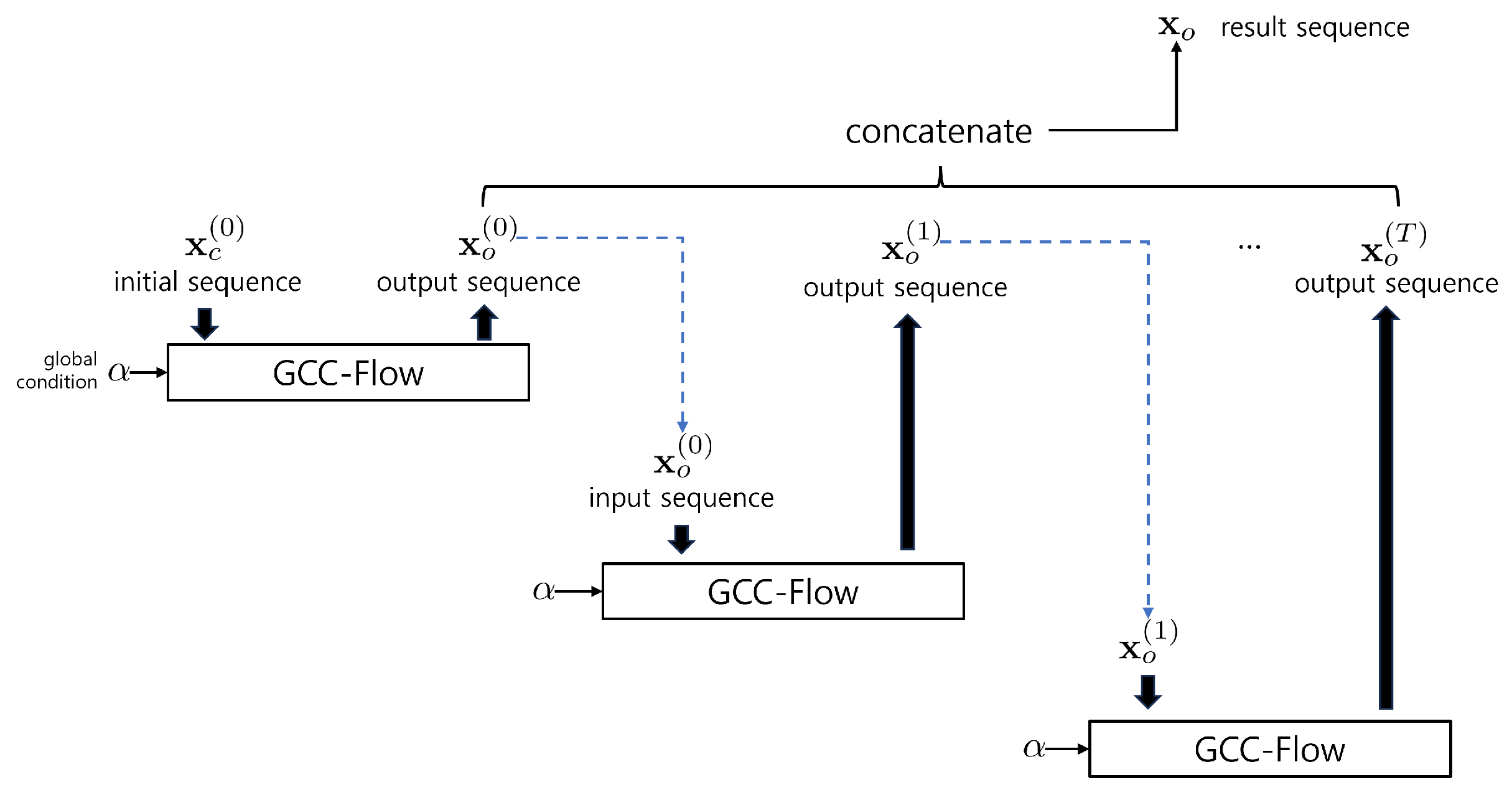
Figure 1 illustrates the autoregressive use of the proposed Globally Conditioned Conditional FLOW (GCC-FLOW ) in order to generate long data sequences. GCC-FLOW generates a sequence

x_{o} = [x_{o 1}, \dots, x_{o L}]

given a conditional sequence

x_{c} = [x_{c 1}, \dots, x_{c L}]

following a conditional distribution

p^{*} (x_{o} | x_{c}; α)

parameterized by a global conditional variable

α \in [0, 1]

. The conditional pdf

p^{*} (x_{o} | x_{c}; α)

is learned by GCC-FLOW to approximate the conditional distribution of the successive data

[x_{L + 1 + k}, \dots x_{2 L + k}]

given

[x_{1 + k}, \dots x_{L + k}]

for

k = 0 \dots

. Given the initial sequence

x_{c}^{(0)}

from the data,

x_{o}^{(0)}

is generated by the GCC-FLOW and

x_{o}^{(k)}

is used as the condition sequence for

x_{o}^{(k + 1)}

for

k = 0, 1, \dots

. The joint distribution of the concatenated sample sequence

x = [x_{o}^{(0)}, x_{o}^{(1)}, \dots, x_{o}^{(T)}]

satisfies

p (x_{o}^{(0)}, x_{o}^{(1)}, \dots, x_{o}^{(T)}) = \prod_{K = 0}^{T} p (x_{o}^{(k)} | x_{o}^{(k - 1)}, \dots, x_{o}^{(1)})

(1)

\begin{matrix} \approx \prod_{K = 0}^{T} p (x_{o}^{(k)} | x_{o}^{(k - 1)}), \end{matrix}

(2)

assuming the block Markov property,

\begin{matrix} p (x_{N + L + 1}, \dots, x_{N + 2 L} | x_{0}, \dots, x_{N + L}) \approx p (x_{N + L + 1}, \dots, x_{N + 2 L} | x_{N + 1}, \dots x_{N + L}) . \end{matrix}

(3)

Since each conditional distribution

p (x_{o}^{(k)} | x_{o}^{(k - 1)})

is approximated by

p^{*} (x_{o}^{(k)} | x_{o}^{(k - 1)})

learned from GCC-FLOW , the joint distribution

x = [x_{o}^{(0)}, x_{o}^{(1)}, \dots, x_{o}^{(T)}]

generated by the GCC-FLOW autoregressively approximates the true data distribution as desired.

2.2. Architecture of GCC-FLOW

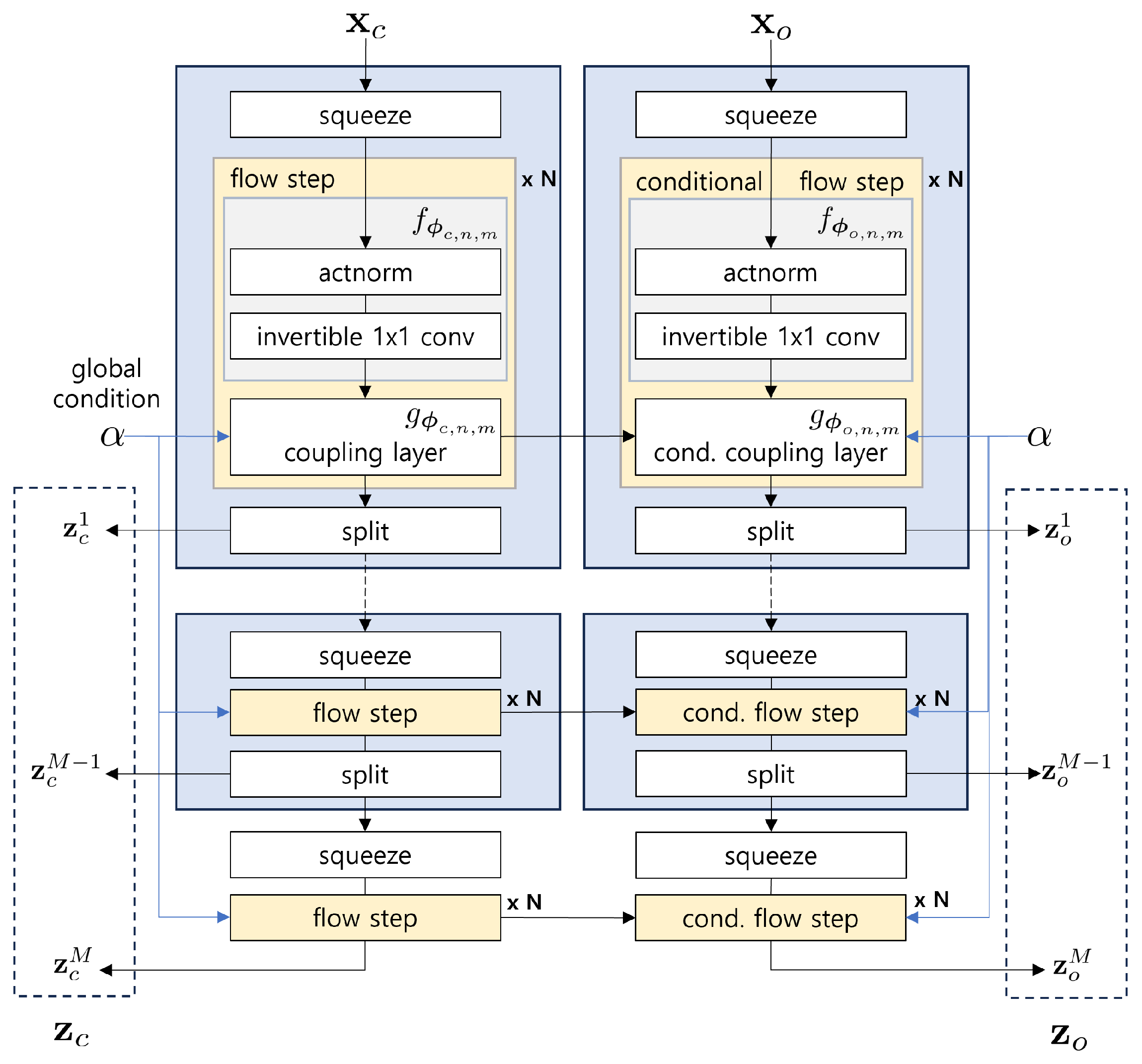
The structure of GCC-FLOW is similar to conditional-FLOW [26] except that the global condition variable

α

is fed into the coupling layer in the FLOW step as shown in Figure 2. GCC-FLOW consists of a pair of FLOW networks, the condition part and the output part, which basically has two identically independent deep network structures that are used repeatedly in the multi-scale frame;

f_{ϕ_{a, n, m}}

and

g_{ψ_{a, n, m}}

, parameterized by the network weights

ϕ_{a, n, m}

and

ψ_{a, n, m},

respectively, where

m = 1, \dots, M

is the index for multi-scale stages and

n = 1, \dots, N

is the index for flow steps in a multi-scale stage, and

a = c

for the condition part and

a = o

for the output part.

In each flow step,

x_{c}

and

x_{o}

are updated as the following

\begin{matrix} {\bar{x}}_{c} & = f_{ϕ_{c, n, m}} (x_{c}^{n}) \end{matrix}

(4)

\begin{matrix} {\bar{x}}_{o} & = f_{ϕ_{o, n, m}} (x_{o}^{n}) \end{matrix}

(5)

\begin{matrix} (s_{c}, b_{c}) & = g_{ϕ_{c, n, m}} ({\bar{x}}_{c}^{u p}, α) \end{matrix}

(6)

\begin{matrix} (s_{o}, b_{o}) & = g_{ϕ_{o, n, n}} ({\bar{x}}_{o}^{u p}, {\bar{x}}_{c}^{u p}, α) \end{matrix}

(7)

\begin{matrix} x_{c}^{n + 1} & = [{\bar{x}}_{c}^{u p}, s_{c} ⊙ {\bar{x}}_{c}^{d o w n} + b_{c}] \end{matrix}

(8)

\begin{matrix} x_{o}^{n + 1} & = [{\bar{x}}_{o}^{u p}, s_{o} ⊙ {\bar{x}}_{o}^{d o w n} + b_{o}] \end{matrix}

(9)

where ⊙ is element-wise multiplication and

({\bar{x}}_{c}^{u p}

{\bar{x}}_{c}^{d o w n}), ({\bar{x}}_{o}^{u p}, {\bar{x}}_{o}^{d o w n})

are the result of halving the channel of

{\bar{x}}_{c}, {\bar{x}}_{o}

, respectively.

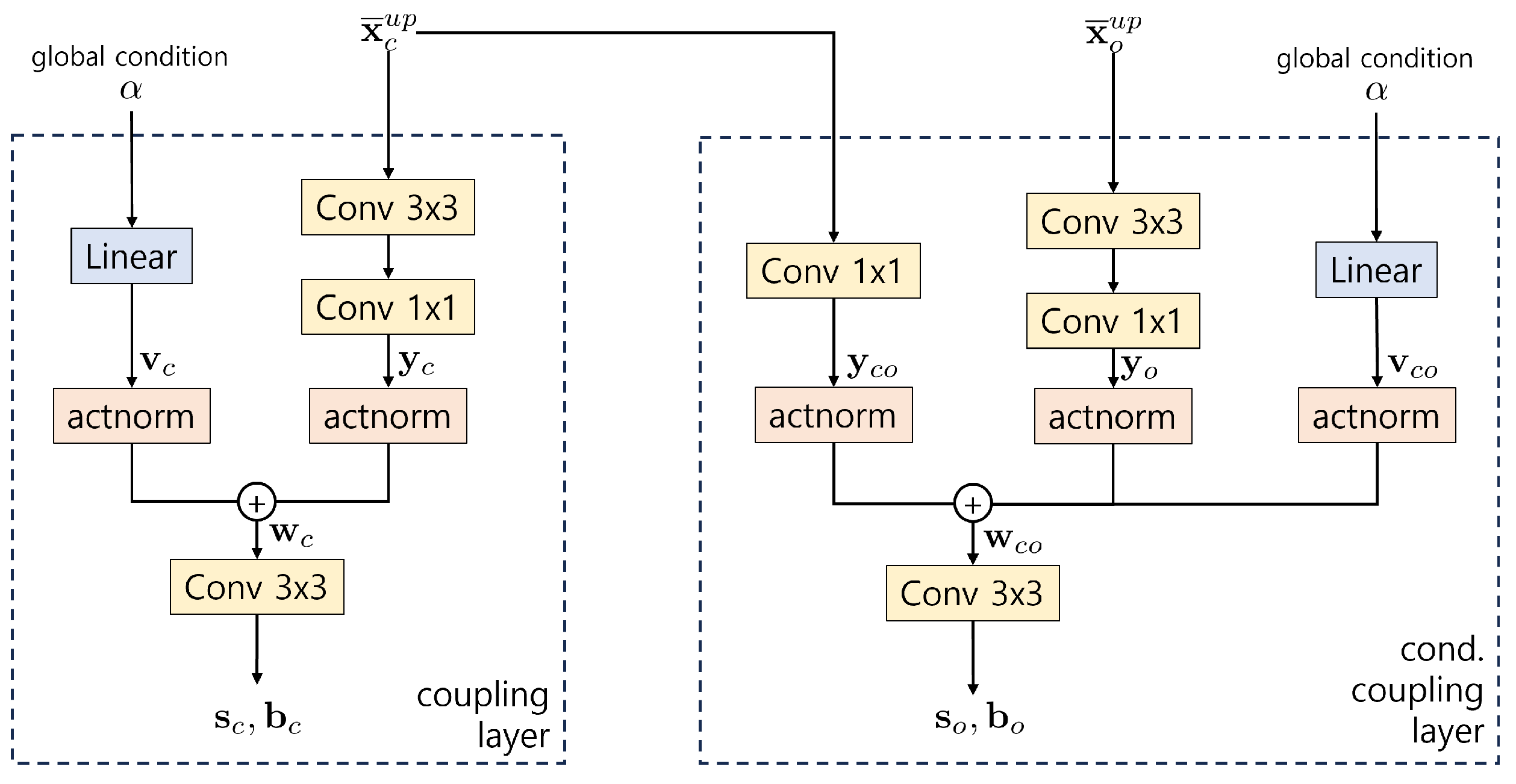
The structure of the coupling layer function

g_{c}

and the conditional coupling layer function

g_{o}

is described in Figure 3. The input tensors

{\bar{x}}_{c}^{u p}

and

{\bar{x}}_{o}^{u p}

, both of size

c \times ℓ

, are converted to the

C_{c o u p l i n g} \times ℓ

tensors, denoted by

y_{c}

y_{c o}

, and

y_{o}

, by convolution networks. The global variable

α \in [0, 1]

is multiplied by a linear weight

v_{a}

of size

1 \times ℓ

(

a \in \{c, o\}

). These two tensors,

v_{o}

and

v_{c}

, are properly scaled and added channel-wise via actnorm. For example, in the coupling layer part,

\begin{matrix} {w_{c}}_{i} = a_{i} {y_{c}}_{i} + b_{i} + a_{0} v_{c} α + b_{0} for i = 1, \dots, C_{c o u p l i n g}, \end{matrix}

(10)

where

w_{c}

denote the intermediate output tensor of the size

C_{c o u p l i n g} \times ℓ

and

w_{c i}

is the i-th channel vector of

w_{c}

and

\{a_{i}, b_{i} | i = 1, \dots, C_{c o u p l i n g}\}

are the actnorm parameters for

v_{c}

and

a_{0}, b_{0}

are the actnorm parameters for

v_{a} α

. Finally,

w_{c}

is processed through a convolution network to restore the original size

c

and split it in half channel-wise to produce

s_{c}

and

b_{c}

At each multi-scale stage, the output

x_{a}^{m N}

is split in half channel-wise, and the first half becomes the m-th stage output,

z_{a}^{m}

, and the remaining half is squeezed, i.e., the length is reduced by half and the channel size is doubled, and fed into the next flow step. Note that in this split-squeeze setting the length of

z_{c}^{k}

at each multi-scale stage becomes

2^{- k} L

, where L is the input length of GCC-FLOW .

In the training phase, networks are trained for

z_{c}^{k}

to be i.i.d. Gaussian,

z_{a}^{k} \sim N (0, I_{L 2^{- k}})

, and in the generation phase the sampled

z_{a}^{k}

from i.i.d. Gaussian

N (0, I_{L 2^{- k}})

are used as input to the inverse network of GCC-FLOW , which is canonically given by the structure of FLOW [27].

3. Experiment Settings

3.1. Data Set

The sea clutter data used in the experiments come from the Dartmouth and Grimbsby databases collected by the IPIX radar [29]. The following two data datasets are used:

1): High sea state data: The 3rd range bin of the data file #269 at Dartmouth labeled as high. The average wave height is 1.8m (max 2.9m)
2): Low sea state data: The 5th range bin of the data file #287 at Dartmouth labeled as low. The average wave height is 0.8m (max 1.3m)

All the data samples are complex-valued and the length of the high sea state data and the low sea state data is

131, 072

. The detailed specification of the data, such as resolution and sampling rate, can be found in [29].

3.2. GCC-FLOW Settings

The length of

x_{o}

and

x_{c}

is set to 512, i.e.

L = 512

, and the height of the clutter data and is set to 2, i.e.,

C = 2

, since the data represent single range bin complex data. The number of multiscale stages of GCC-FLOW is set to 4, i.e.,

M = 4

and in a multiscale stage the number of FLOW iterations is set to

N = 4

. The channel size in the coupling layer is

C_{c o u p} = 32

. The model is trained on NVIDIA RTX 3090 with a learning rate of

3 \times 10^{- 4}

, batch size of 4, and trained on 512 randomly selected sequences with length of 1024 by randomly sampled starting points.

4. Experiment Results

4.1. Sea Clutter Augmentation Using GCC-FLOW

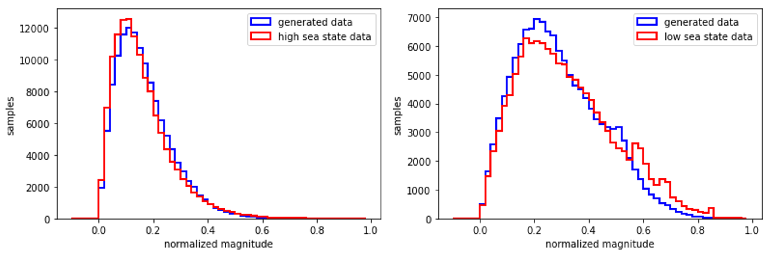
Figure 4 compares the magnitude histogram of the generated sea clutter data by the GCC-FLOW trained on the high sea state data and on the low sea state data, respectively, with the magnitude histograms of the original data. Figure 5 compares the magnitude autocorrelation of the generated sea clutter data by the GCC-FLOW trained on the high sea state data and on the low sea state data, respectively, with that of the original high sea state and the low sea sate data, where the magnitude autocorrelation is defined as

\begin{matrix} ρ (s) = \frac{\sum_{l = 1}^{L - s} (| x_{l} | - \bar{x}) (| x_{l + s} | - \bar{x})}{\sum_{l = 1}^{L} {(| x_{l} | - \bar{x})}^{2}}, \end{matrix}

(11)

where

\bar{x} = \frac{1}{L} \sum_{l = 1}^{L} | x_{l} |

s = 0, \dots, L

, and L is set to 512.

The GCC-FLOW is trained using 256 blocks of 512 consecutive samples (131,072 training samples in total) with the global condition variable

α

set to 0. GCC-FLOW generates 262,144 consecutive samples and the first 131,072 samples are used to plot the histogram and the autocorrelation function.

To confirm that the generated samples have the same statistical properties at each time point, consecutive

10, 000

samples are taken from the beginning (

1 \sim 10, 000

), from the middle (

13, 0001 \sim 14, 000

), and from the end (

25, 2145 \sim 26, 2144

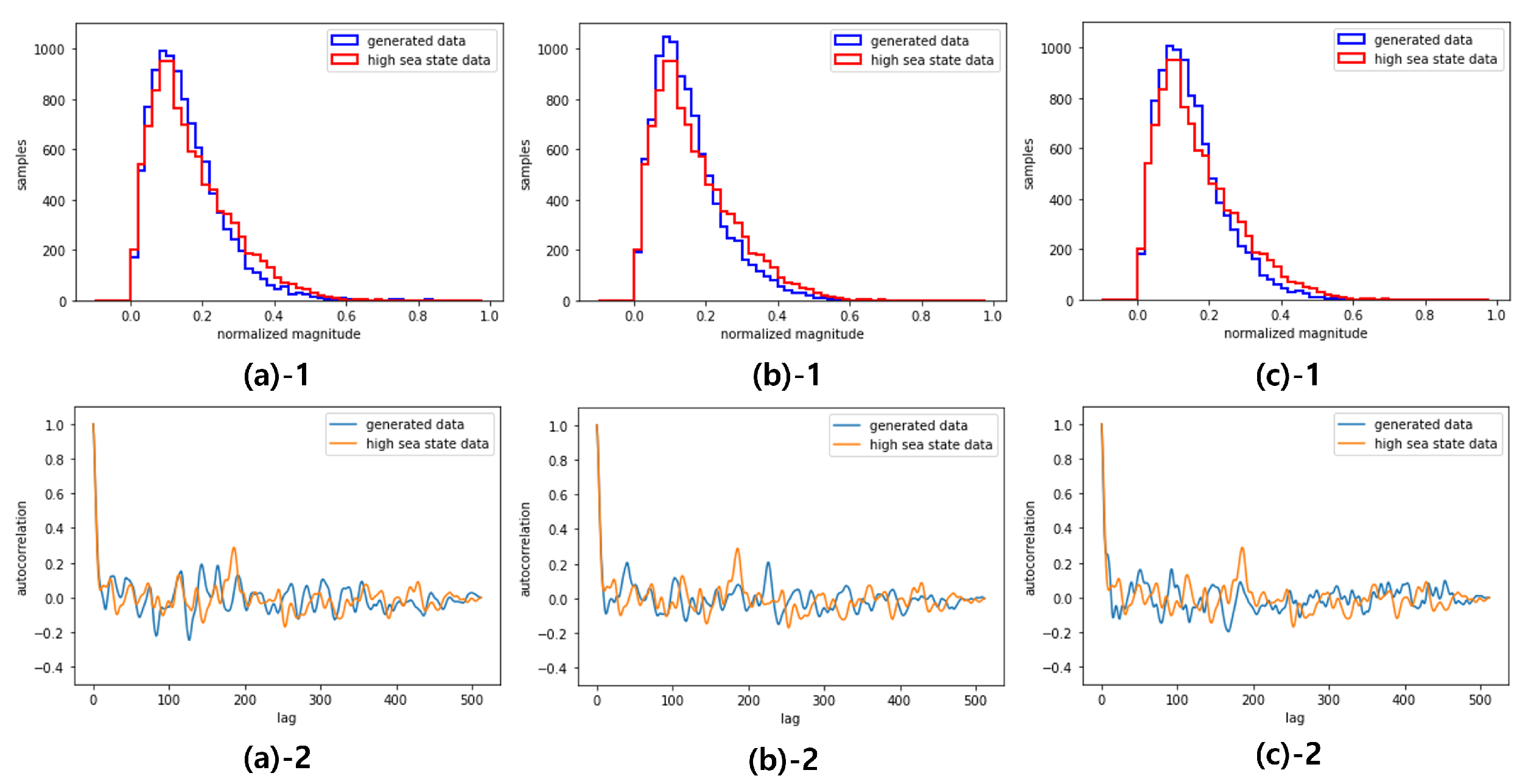
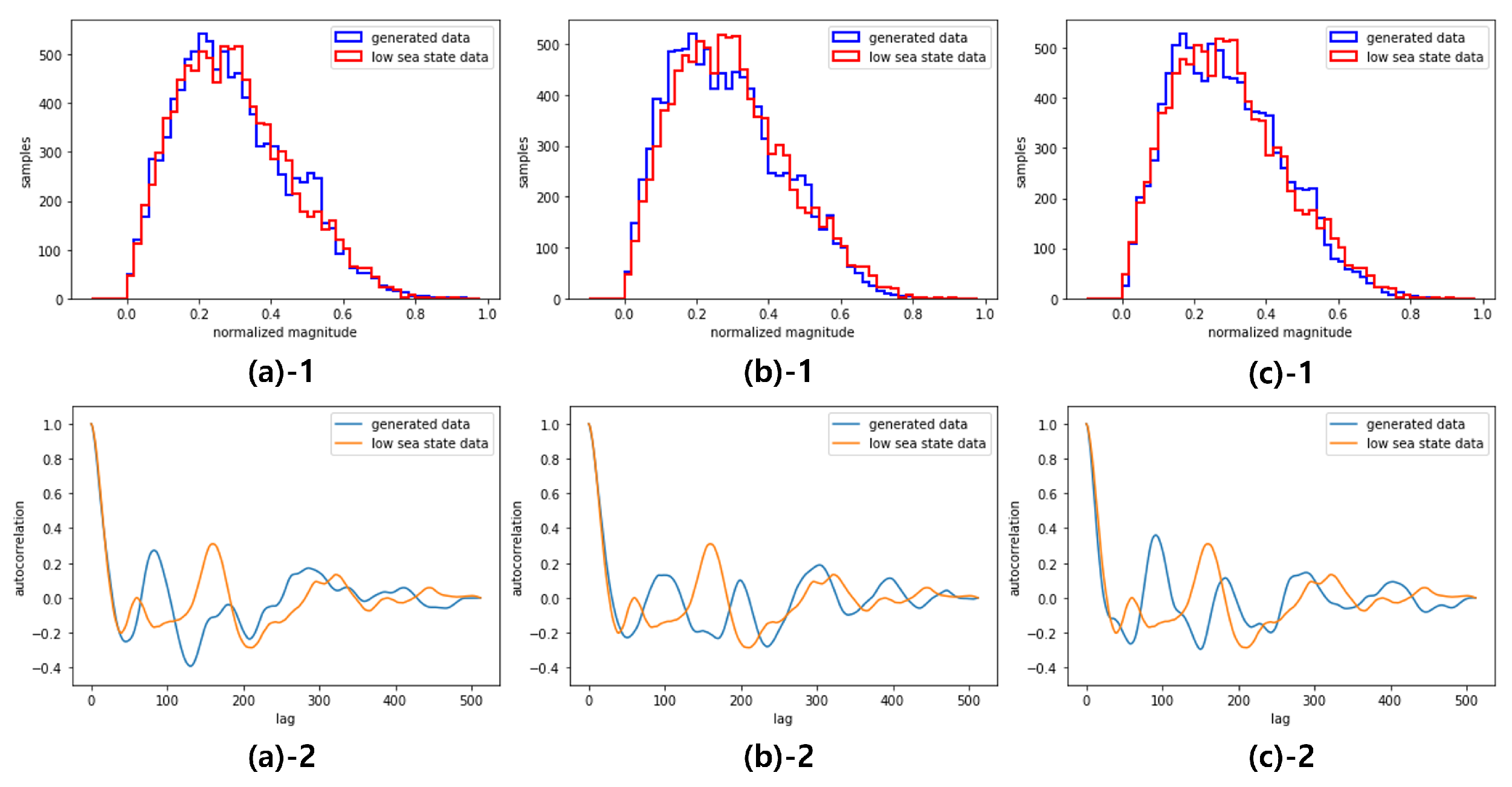
). Figure 6 and Figure 7 show the magnitude histogram and the magnitude autocorrelation of the generated sea clutter data using GCC-FLOW trained from the high sea state data and the low sea state data, respectively, at the three time points. Note that the characteristic of the high sea data (concentrated distribution and high frequency fluctuation in correlation) and the characteristic of the low sea data (spread distribution and low frequency fluctuation in correlation) are preserved in all time points.

4.2. Sea Clutter generation using GCC-FLOW with global condition

Using the global condition variable

α

, a single GCC-FLOW can be trained on two different datasets; high sea state data with

α = 1

and low sea state data with

α = 0

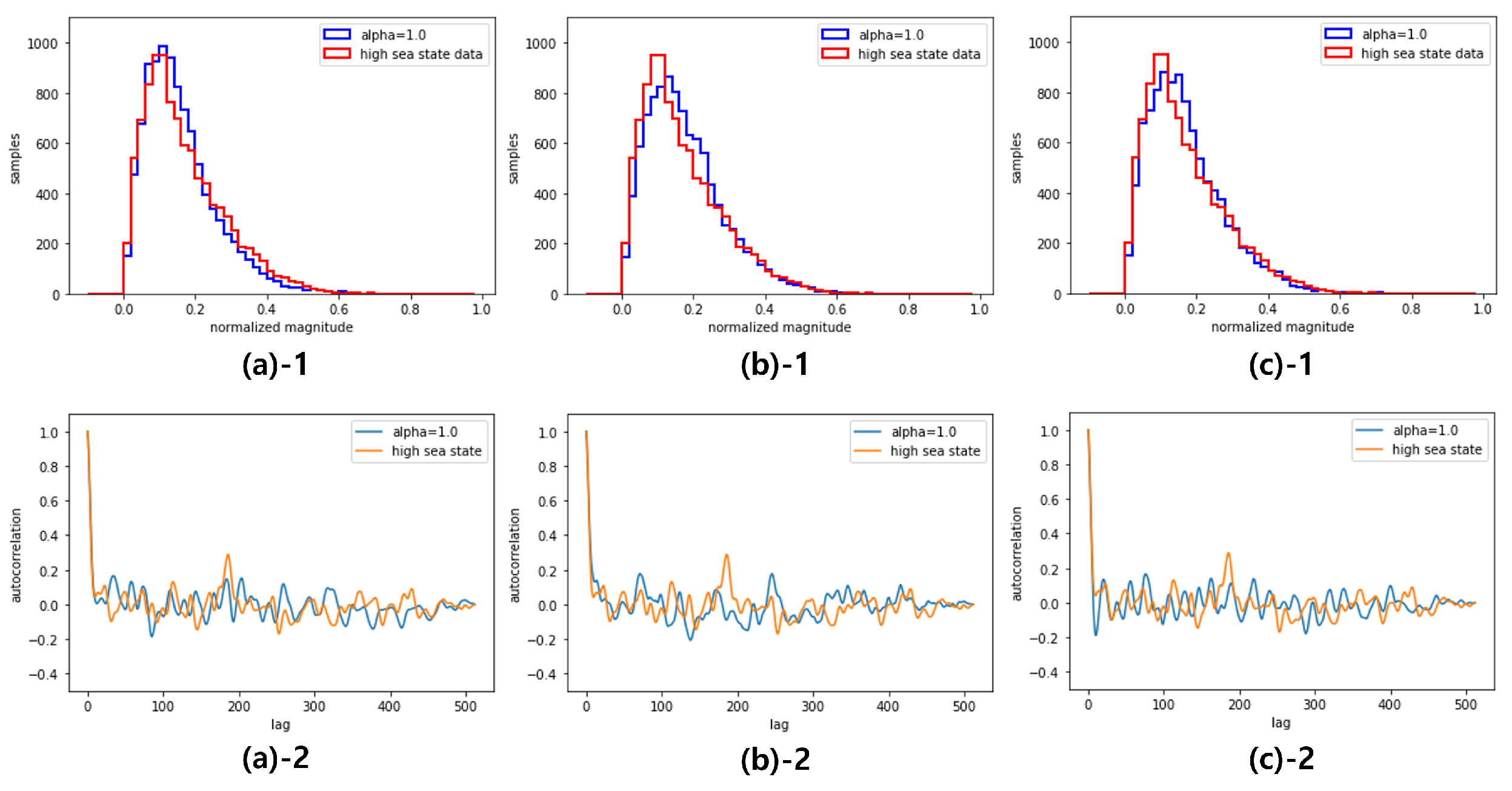
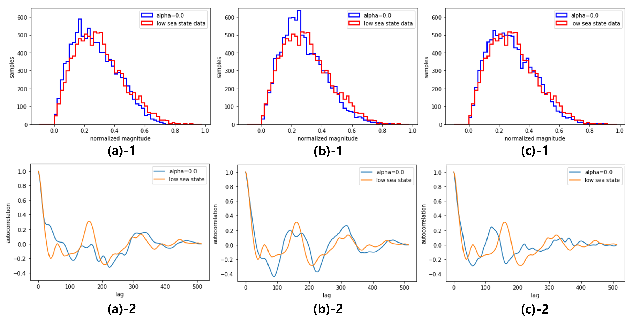
. Figure 8 and Figure 9 plot the magnitude histogram and magnitude autocorrelation of the generated sea clutter data using GCC-FLOW with

α = 1

and

α = 0

, respectively, at the three different time points (beginning, middle, and end) from the

262, 144

samples.

The benefit of this single mode training on two different datasets is the feature interpolation, i.e., by adjusting

α

between 0 and 1, the GCC-FLOW can generate data with interpolated statistical characteristics between the high and low sea state. Figure 10 shows the magnitude histogram of generated data for

α = 0.2, 0.5, 0.8

at three different time points (beginning, middle, and end) of

262, 144

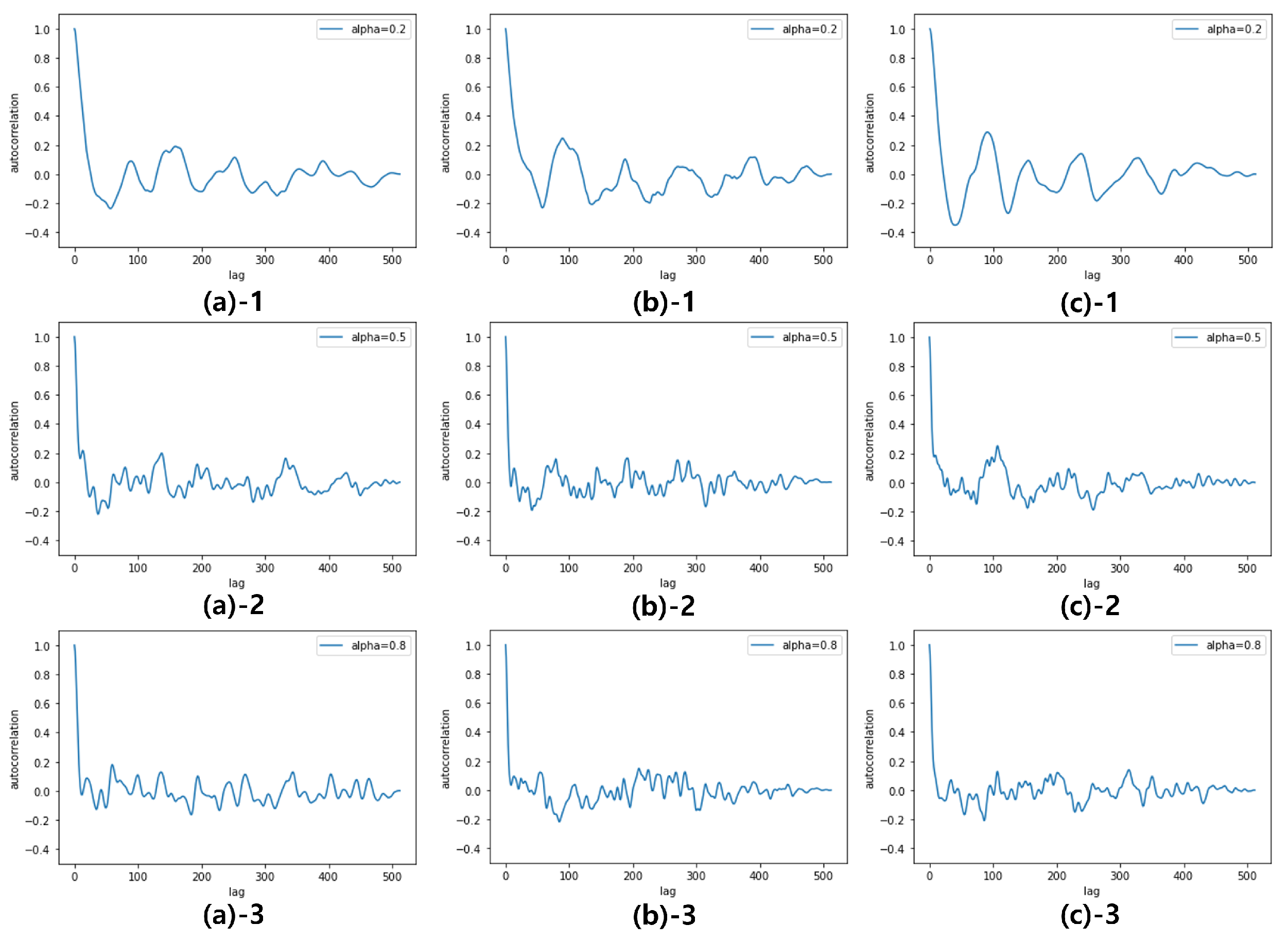
samples. Figure 11 presents the autocorrelation of generated data for

α = 0, 2, 0.5, 0.8

at three different time points (beginning, middle, and end) of

262, 144

samples. In both figures, as

α

increases from 0 to 1 the characteristics of magnitude distribution and autocorrelation transforms from the low sea state characteristics to the high sea state characteristics. This suggests that by using GCC-FLOW with a global condition variable tuned to sea state, various sea state sea clutter can be generated without the need for the dedicated training datasets for different sea states.

5. Conclusions

A novel work, Globally Conditioned Conditional FLOW (GCC-FLOW ), has been proposed for sea clutter data augmentation due to the expensive and time-consuming nature of acquiring the desired sea clutter data. Experimental results show that GCC-FLOW successfully generates sequences of arbitrary length with the same statistical properties of the given sea clutter data, in contrast to the existing block-by-block methods. Moreover, by introducing a global state variable, the proposed GCC-FLOW can generate sea clutter with different sea state by feature interpolation without requiring the training data with a target feature.

Funding

This study is the result of research funded by the Agency for Defense Development (contract number UI220077JD).

Institutional Review Board Statement

Not Applicable

Informed Consent Statement

Not Applicable

Data Availability Statement

The data presented in this study are available on http://soma.ece.mcmaster.ca/ipix/index.html

Conflicts of Interest

The authors declare no conflicts of interest.

References

K. D. Ward, R.J.A.T.; Watts, S. Sea clutter: Scattering, the K distribution and radar performance. Waves in Random and Complex Media 2007, 17, 233–234. [CrossRef]
E. Conte, M.L. Characterisation of radar clutter as a spherically invariant random process. IEE Proceedings F (Communications, Radar and Signal Processing) 1987, 134, 191–197(6). [CrossRef]
Rangaswamy, M.; Weiner, D.; Ozturk, A. Computer generation of correlated non-Gaussian radar clutter. IEEE Transactions on Aerospace and Electronic Systems 1995, 31, 106–116. [Google Scholar] [CrossRef]
Barnard, T.; Weiner, D. Non-Gaussian clutter modeling with generalized spherically invariant random vectors. IEEE Transactions on Signal Processing 1996, 44, 2384–2390. [Google Scholar] [CrossRef]
Armstrong, B.; Griffiths, H. Modelling spatially correlated K-distributed clutter. Electronics Letters 1991, 27, 1355–1356. [Google Scholar] [CrossRef]
Wang, J.; Xu, X. Simulation of Correlated Low-Grazing-Angle Sea Clutter Based on Phase Retrieval. IEEE Transactions on Geoscience and Remote Sensing 2015, 53, 3917–3930. [Google Scholar] [CrossRef]
Goldstein, H. Sea echo. In Propagation of Short Radio Waves; McGraw-Hill New York, 1951; Vol. 13, pp. 481–527.
Trunk, G.V.; George, S.F. Detection of Targets in Non-Gaussian Sea Clutter. IEEE Transactions on Aerospace and Electronic Systems 1970, AES-6, 620–628. [Google Scholar] [CrossRef]
Jakeman, E.; Pusey, P. A model for non-Rayleigh sea echo. IEEE Transactions on Antennas and Propagation 1976, 24, 806–814. [Google Scholar] [CrossRef]
Matsuo Sekine, Y.H.M. Weibull Radar Clutter; Radar, Sonar and Navigation, Institution of Engineering and Technology, 1990.
Ishikawa, Y.; Sekine, M.; Musha, T. Observation of k-distributed sea clutter via an x-band radar. Electronics and Communications in Japan (Part I: Communications) 1994, 77, 72–82. [Google Scholar] [CrossRef]
Bouvier, C.; Martinet, L.; Favier, G.; Artaud, M. Simulation of radar sea clutter using autoregressive modelling and K-distribution. Proceedings International Radar Conference, 1995, pp. 425–430. [CrossRef]
Middleton, D. New physical-statistical methods and models for clutter and reverberation: the KA-distribution and related probability structures. IEEE Journal of Oceanic Engineering 1999, 24, 261–284. [Google Scholar] [CrossRef]
Rosenberg, L.; Crisp, D.J.; Stacy, N.J. Analysis of the KK-distribution with X-band medium grazing angle sea-clutter. 2009 International Radar Conference "Surveillance for a Safer World" (RADAR 2009), 2009, pp. 1–6.
Dong, Y. Distribution of X-band high resolution and high grazing angle sea clutter; Citeseer, 2006.
FARSHCHIAn, M.; Posner, F.L. The Pareto distribution for low grazing angle and high resolution X-band sea clutter. 2010 IEEE Radar Conference. IEEE, 2010, pp. 789–793.
Bocquet, S. Simulation of correlated Pareto distributed sea clutter. 2013 International Conference on Radar, 2013, pp. 258–261. [CrossRef]
Tough, R.J.A.; Ward, K.D. The correlation properties of gamma and other non-Gaussian processes generated by memoryless nonlinear transformation. Journal of Physics D: Applied Physics 1999, 32, 3075. [Google Scholar] [CrossRef]
Watts, S.; Rosenberg, L. Challenges in radar sea clutter modelling. IET Radar, Sonar & Navigation 2022, 16, 1403–1414. [Google Scholar]
Lample, G.; Zeghidour, N.; Usunier, N.; Bordes, A.; Denoyer, L.; Ranzato, M. Fader networks: Manipulating images by sliding attributes. Advances in neural information processing systems 2017, 30.
He, Z.; Zuo, W.; Kan, M.; Shan, S.; Chen, X. AttGAN: Facial Attribute Editing by Only Changing What You Want. IEEE Transactions on Image Processing 2019, 28, 5464–5478. [Google Scholar] [CrossRef] [PubMed]
Bin DING, Xue XIA, X.L. Sea Clutter Data Augmentation Method Based on Deep Generative Adversarial Network. Journal of Electronics and Information Technology 2021, 43, 1985. [Google Scholar]
Zhang, X.; Wang, Z.; Lu, K.; Pan, Q.; Li, Y. Data Augmentation and Classification of Sea-Land Clutter for Over-the-Horizon Radar Using AC-VAEGAN. IEEE Transactions on Geoscience and Remote Sensing 2023. [Google Scholar] [CrossRef]
Bengio, Y.; Simard, P.; Frasconi, P. Learning long-term dependencies with gradient descent is difficult. IEEE Transactions on Neural Networks 1994, 5, 157–166. [Google Scholar] [CrossRef] [PubMed]
Pascanu, R.; Mikolov, T.; Bengio, Y. On the difficulty of training recurrent neural networks. Proceedings of the 30th International Conference on Machine Learning; Dasgupta, S.; McAllester, D., Eds.; PMLR: Atlanta, Georgia, USA, 2013; Vol. 28, Proceedings of Machine Learning Research, pp. 1310–1318.
Pumarola, A.; Popov, S.; Moreno-Noguer, F.; Ferrari, V. C-flow: Conditional generative flow models for images and 3d point clouds. Proceedings of the IEEE/CVF Conference on Computer Vision and Pattern Recognition, 2020, pp. 7949–7958.
Kingma, D.P.; Dhariwal, P. Glow: Generative flow with invertible 1x1 convolutions. Advances in neural information processing systems 2018, 31.
Carretero-Moya, J.; Gismero-Menoyo, J.; Blanco-del Campo, A.; Asensio-Lopez, A. Statistical Analysis of a High-Resolution Sea-Clutter Database. IEEE Transactions on Geoscience and Remote Sensing 2010, 48, 2024–2037. [Google Scholar] [CrossRef]
Ipix radar website. http://soma.ece.mcmaster.ca/ipix/dartmouth/index.html.

Figure 1. Autoregressive generation using GCC-FLOW

Figure 2. Architecture of GCC-FLOW

Figure 3. Architecture of coupling networks in GCC-FLOW

Figure 4. Magnitude distribution the generated data by GCC-FLOW in comparison with the true data: high sea state(left), low sea state(right)

Figure 5. Autocorrelation of the generated data by GCC-FLOW in comparison with the true data: high sea state(left), low sea state(right)

Figure 6. Distribution(1) and Autocorrelation(2) of the generated data trained on high sea state data: beginning(a), middle(b), end(c)

Figure 7. Distribution(1) and Autocorrelation(2) of the generated data trained on low sea state data: beginning(a), middle(b), end(c)

Figure 8. Distribution(1) and Autocorrelation(2) of the generated data by GCC-FLOW with

α = 1

: beginning(a), middle(b), end(c)

Figure 8. Distribution(1) and Autocorrelation(2) of the generated data by GCC-FLOW with

α = 1

: beginning(a), middle(b), end(c)

Figure 9. Distribution(1) and Autocorrelation(2) of the generated data by GCC-FLOW with

α = 0

: beginning(a), middle(b), end(c)

Figure 9. Distribution(1) and Autocorrelation(2) of the generated data by GCC-FLOW with

α = 0

: beginning(a), middle(b), end(c)

Figure 10. Interpolated distribution by the global condition variable

α =

0.2, 0.5, 0.8 : beginning(a), middle(b), end(c)

Figure 10. Interpolated distribution by the global condition variable

α =

0.2, 0.5, 0.8 : beginning(a), middle(b), end(c)

Figure 11. Interpolated autocorrelation by the global condition variable

α =

0.2(1), 0.5(2), 0.8(3) : beginning(a), middle(b), end(c)

Figure 11. Interpolated autocorrelation by the global condition variable

α =

0.2(1), 0.5(2), 0.8(3) : beginning(a), middle(b), end(c)

Disclaimer/Publisher’s Note: The statements, opinions and data contained in all publications are solely those of the individual author(s) and contributor(s) and not of MDPI and/or the editor(s). MDPI and/or the editor(s) disclaim responsibility for any injury to people or property resulting from any ideas, methods, instructions or products referred to in the content.

© 2024 by the authors. Licensee MDPI, Basel, Switzerland. This article is an open access article distributed under the terms and conditions of the Creative Commons Attribution (CC BY) license (http://creativecommons.org/licenses/by/4.0/).

Copyright: This open access article is published under a Creative Commons CC BY 4.0 license, which permit the free download, distribution, and reuse, provided that the author and preprint are cited in any reuse.

MDPI Initiatives

Important Links

Choose an area of interest and we will send you notifications of new preprints at your preferred frequency.

Disclaimer

Globally Conditioned Conditional FLOW (GCC-FLOW) for Sea Clutter Data Augmentation

Abstract

1. Introduction

2. Methods

2.1. Autoregressive Data Generation Using GCC-FLOW

2.2. Architecture of GCC-FLOW

3. Experiment Settings

3.1. Data Set

3.2. GCC-FLOW Settings

4. Experiment Results

4.1. Sea Clutter Augmentation Using GCC-FLOW

4.2. Sea Clutter generation using GCC-FLOW with global condition

5. Conclusions

Funding

Institutional Review Board Statement

Informed Consent Statement

Data Availability Statement

Conflicts of Interest

References

MDPI Initiatives

Important Links

Subscribe