1. Introduction
The e-commerce sector is in a constant state of growth and evolution, particularly within its subdomain of online food delivery (OFD) [
1,
2]. Recent market forecasts indicate a steady rise in revenue for companies offering such services. With numerous players in the market, ensuring customer satisfaction is paramount for a company’s survival. Customers increasingly demand user-friendly applications that simplify the ordering process with just a few taps, while also providing features such as delivery time estimates and communication channels with couriers [
3]. However, estimating delivery times accurately without real-time data presents a significant challenge. While companies can track courier positions via GPS, they lack access to real-time information on factors such as traffic, accidents, and roadworks.
To address the challenge of insufficient real-world data, companies employ a diverse array of statistical and machine learning techniques to infer delivery times. Among these methods, neural networks, including Deep Neural Networks (DNNs), Convolutional Neural Networks (CNNs), Recurrent Neural Networks (RNNs), and Long Short-Term Memory networks (LSTMs), are prominently utilized [
4]. Additionally, specialized expert systems tailored to specific cities or geographic regions are commonly developed.
Although Bayesian statistics and inference have gained increasing popularity, there remains a notable scarcity of articles addressing their application in delivery time prediction. The method boasts several advantages: it offers straightforward, interpretable models, the capacity to adapt and improve with new data, and provides a measure of uncertainty for each prediction. However, it also presents challenges, notably its computational demands and the potential for poor model performance due to incorrect assumptions.
This article introduces two Bayesian models designed for predicting food delivery times. Utilizing a linear combination of predictor variables, we generate practical range of outputs. These models offer a balance of generality and adaptability, allowing for tuning with expert knowledge. This ensures flexibility and stability in various contexts. To assess their performance and identify any potential drawbacks, we compared the models using the PSIS-LOO and WAIC criteria.
The main contributions of this paper are as follows: (1) To the best of our knowledge, this is the first application of Bayesian inference to online food delivery time prediction. (2) By specifying models as a linear combination of predictors, we achieve high interpretability, which aids in identifying the primary factors influencing delivery time. (3) Our results indicate that Bayesian inference holds promise for further exploration in this context, as it can lead to promising results.
The remainder of this paper is structured as follows: In the next section, relevant studies in the extant literature are reviewed and discussed.
Section 3.1 provides a short introduction into concept of Bayesian statistics.
Section 3.2 refers to numerical computation methods utilized in our work.
Section 3.3 reveals data source and contains reference to part 1 of this article, where preprocessing was described.
Section 3.4 focuses on models definition, prior distributions selection and prior predictive checks. In
Section 4, we present and explain the results of our work as posterior predictive checks, where
Section 4.1 focuses on model 1 and
Section 4.2 focuses on model 2. In
Section 4.3 we compare models to see how they fare against each other. Finally,
Section 5 summarizes the conclusions drawn from this study.
2. Literature Review
Food delivery time estimation can be perceived in category of Estimated Time of Arrival (ETA). In our work it will also include meal preparation time, but the rest focuses solely on travel time between origin and destination. Overall there are two common approaches to ETA: route-focused and origin-destination focused.
The route-based approach focuses on segmenting route and estimating travel time of each segment. Lee et al. implemented real-time expert system, that takes present and historical data and produces travel time prediction rules via data mining techniques. Also they implement dynamic weight combination governed by meta-rules which allows for real-time road events response to enhance prediction’s precision [
5]. Li et al. proposed deep generative model – DeepGTT. It is a probabilistic model designed to generate travel time distribution, from which travel time as well as uncertainty about it can be inferred [
6]. Asghari et al. presented algorithms for computing probability distribution of travel times for each link of given route. It differs from other works, as authors mention that elsewhere probablistic link travel times are given a priori. This, and the work mentioned beforehand are one of the few works that focuses on distributions, rather than strict numbers [
7]. Wang et al. proposed model for estimating travel time of any path consisting of connected road segments based on current and historical GPS records, as well as map sources. Due to data sparsity (not every road will be travelled by vehicle with GPS) and trade-offs associated with multiple ways of connecting road fragments to form a route the problem as a whole was not solved [
8]. Wang et al. formulate ETA as a spatial-temporal problem. They adapted different neural networks, as well as proposed authorial Wide-Deep-Recurrent model and trained them on floating-car data. Solution showed promising result and was deployed for Didi Chuxing’s vehicle for hire company [
9].
The origin-destination methods refrain from estimating routes, stating that it is time-consuming and potentially erroneus, as well as gives worse result than OD methods. Zhu et al. predict Order Fulfilment Cycle Time (OFCT), which is the time between placing an order and receiving meal. Their approach consists of identification key factors behind OFCT and capturing them within multiple features from diverse data sources, then feeding them to DNN created for this task. It’s worth noting that their approach is specifically tailored to food delivery, which aligns with the common goal outlined in our article.[
10]. Li et al. proposed MURAT model with goal of predicting travel time given origin and destination location, as well as departure time. They also present multi-task learning framework to integrate prior historical data into training process to boost performance [
11]. Wu, C. H. et al. examined classical machine learning algorithm, which is support vector regression. Their findings show feasibility of such method for travel time prediction [
12]. Wang et al. leverage increasing availability of travel data. Their approach is to use large historical datasets to accurately predict travel time between origin and destination without computing route. Shown solution outperformed services of Bing Maps and Baidu Maps at the time [
13].
3. Materials and Methods
3.1. Bayesian Inference
For better understanding of problem formulation and proposed solution a short introduction to Bayesian inference is in order. It is a method of statistical inference, in which we fit a predefined probability model to a set of data and evaluate outcomes with regards to observed parameters of the model and unobserved quantities, like predictions for new data points [
14]. It is done with the use of Bayes’ rule, shown in equation 1
or rewritten in unnormalized version
This tells us the relation between
, which is unobservable vector of variables of interest and
y, which is vector of observed variables. Left hand-side of the equation is called posterior distribution while the right hand-side is product of prior distribution and likelihood function. We define prior predictive distribution as
and posterior predictive distribution as
Prior predictive distribution is not conditional on previous observation
y of the process and refers to observed data, while posterior predictive distribution is conditional on
y and predicts potential future observations
[
14].
3.2. Stan Programming
Models were created in Stan. It is a programming language written in C++ and used for statistical inference. It provides concise way of defining Bayesian models as simple scripts, yet allows for efficient computation of Markov Chain Monte Carlo methods, which are essential part of Bayesian inference [
15].
3.3. Data
Data used for inference comes from kaggle [
16]. Feature selection, preprocessing and data analysis are described in part 1 of this article [
17]. Chosen features are presented in
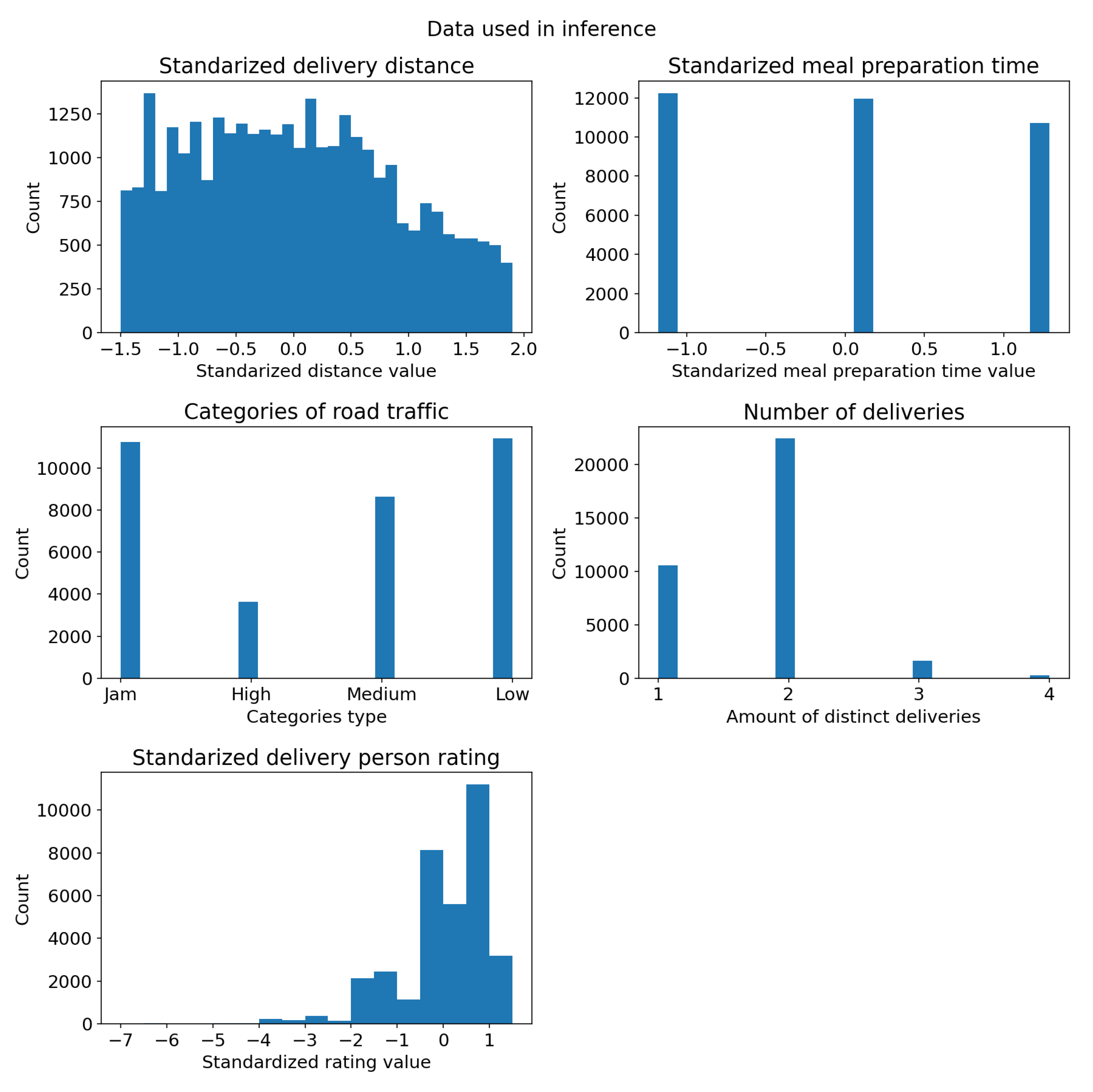
Table 1. There was 45593 raw data samples. After processing we ended with 34920, which will be further denoted as N. Histograms of the data are presented on
Figure 1 [
17].
3.4. Models
Both models are generalized linear models. We have defined linear predictor as
where
X denotes vector of features described in
Table 1 and
B is vector of coefficients. Each coefficient’s distribution is described in appropriate Model section. Both vectors are size Nx1 [
18].
We then used logarithmic link function to transform linear predictor’s domain to positive real numbers. It was one of the possible options, but nevertheless necessary, as both models are defined by inverse gamma function. This way we obtained explanatory variable
, representing mean of the outcome variable [
18]. We defined prior distribution for standard deviation of our models, denoted as
, to be exponential distribution with rate parameter equal 0.5.
Lastly, we defined likelihood as inverse gamma distribution with parameters shape () and scale (), computed from and in such way, that the resulting distribution had mean and standard deviation of and . Reasoning behind this particular distribution was to model skewness of the data effectively. Also, time has to be strictly positive continuous, which inverse gamma also provides.
While models itself were defined in Stan, the experiments were done via CmdStanPy, which is one of Python’s interface for it [
15].
3.4.1. Model 1
First model is defined as follows:
3.4.2. Model 2
Second model is extension of the first model by two predictors: number of deliveries and standardized delivery person rating. As such we only present changes necessary for creating model 2 out of model 1:
Figure 2.
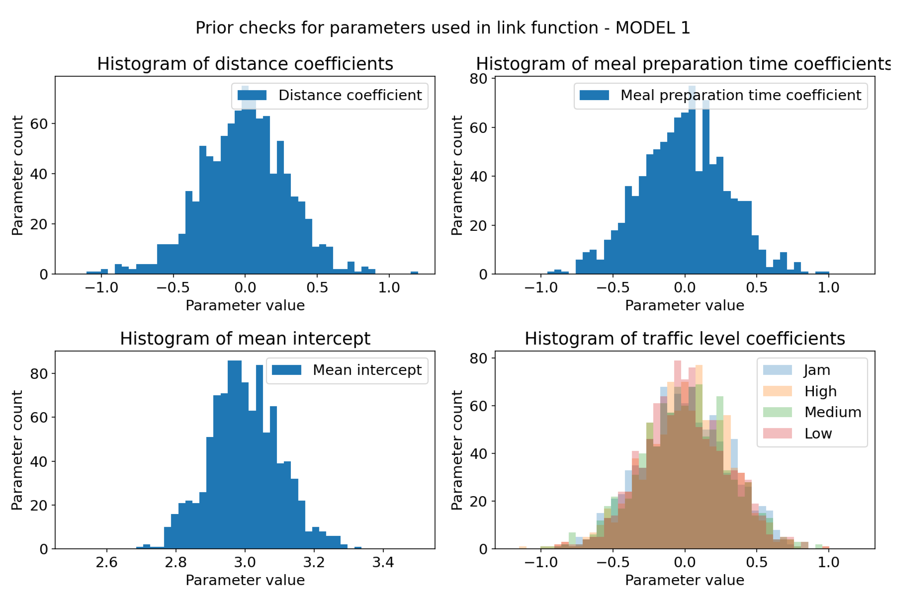
Sampling check for prior distributions of model 1 link function parameters (parameters with _coeff suffix). X-axis represents coefficients values and Y-axis represents sample count. Each of the coefficients follows its distribution, which is necessary for prior check to be successful. (a) Prior distribution of distance coefficient, defined as . (b) Prior distribution of meal preparation time coefficient, defined as . (c) Prior distribution of parameter, defined as . parameter represents our belief of what mean delivery time should be in case all other parameters are 0. (d) Joint plot of prior distributions of traffic level coefficients, all defined as .
Figure 3.
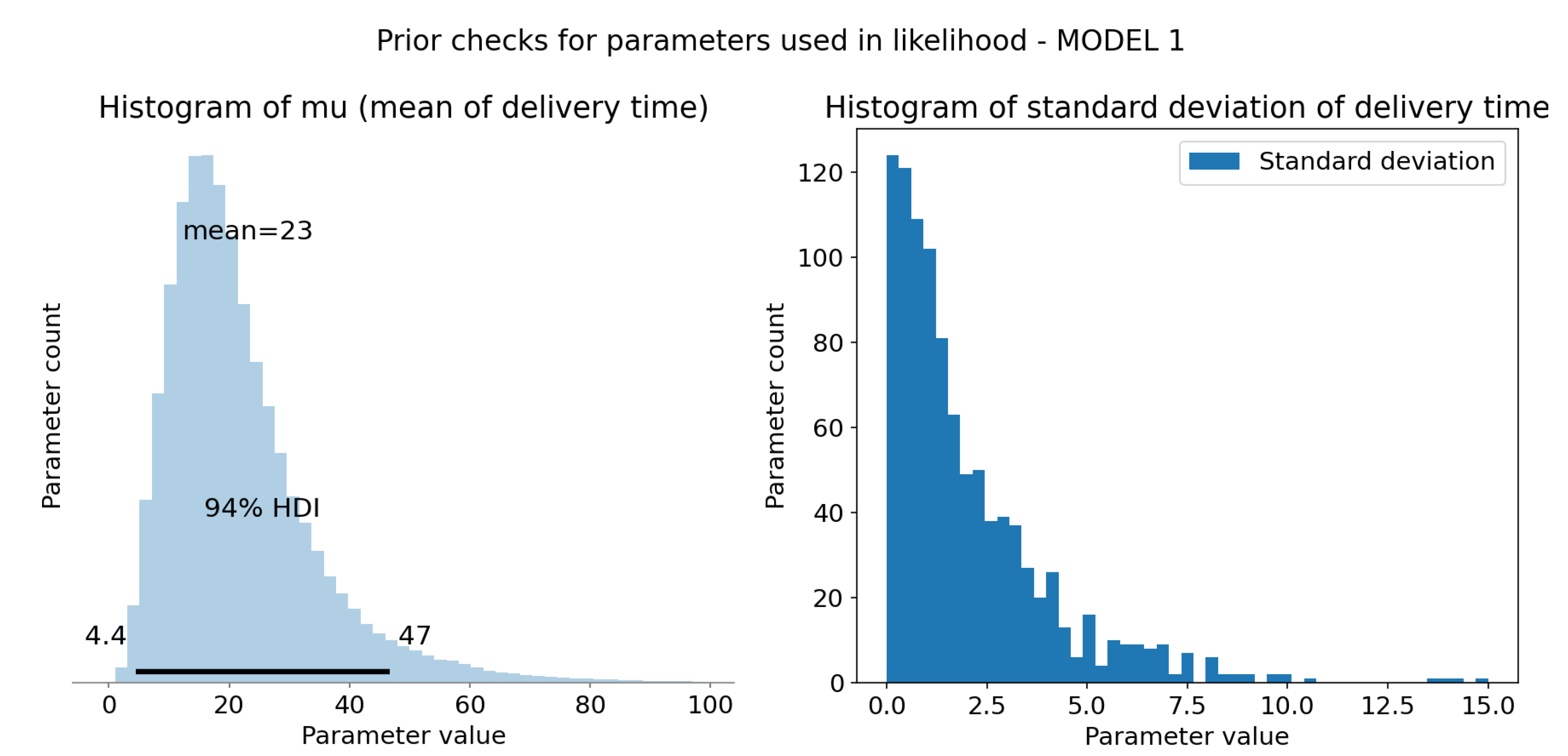
Computation and sample check of model 1 likelihood parameters. X-axis is time in minutes and Y-axis represents sample count. (a) Computed represent mean delivery time for each sample. HDI 94% is represented as black bar at the bottom of the plot and tells us that 94% of shown mean times falls in range 4.4 to 47 minutes. Mean of this distribution (at the top of the plot) is 23 minutes, which is reasonable value. (b) Prior distribution of standard deviation of the model, defined as .
Figure 4.
Prior predictive checks - model 1. (a) HDI 94% is represented as black bar at the bottom of the plot and tells us that 94% of shown mean times falls in range 3.2 to 47 minutes, which is broad range. Mean of this distribution (at the top of the plot) is 23 minutes, which is reasonable value. (b) Real and simulated data overlay. Both are normalized, so that integral of the graph is 1. It was necessary for comparison. Measured data is included within generated data, which means that all observations are possible within prior model. This means that prior checks are successful.
Figure 5.
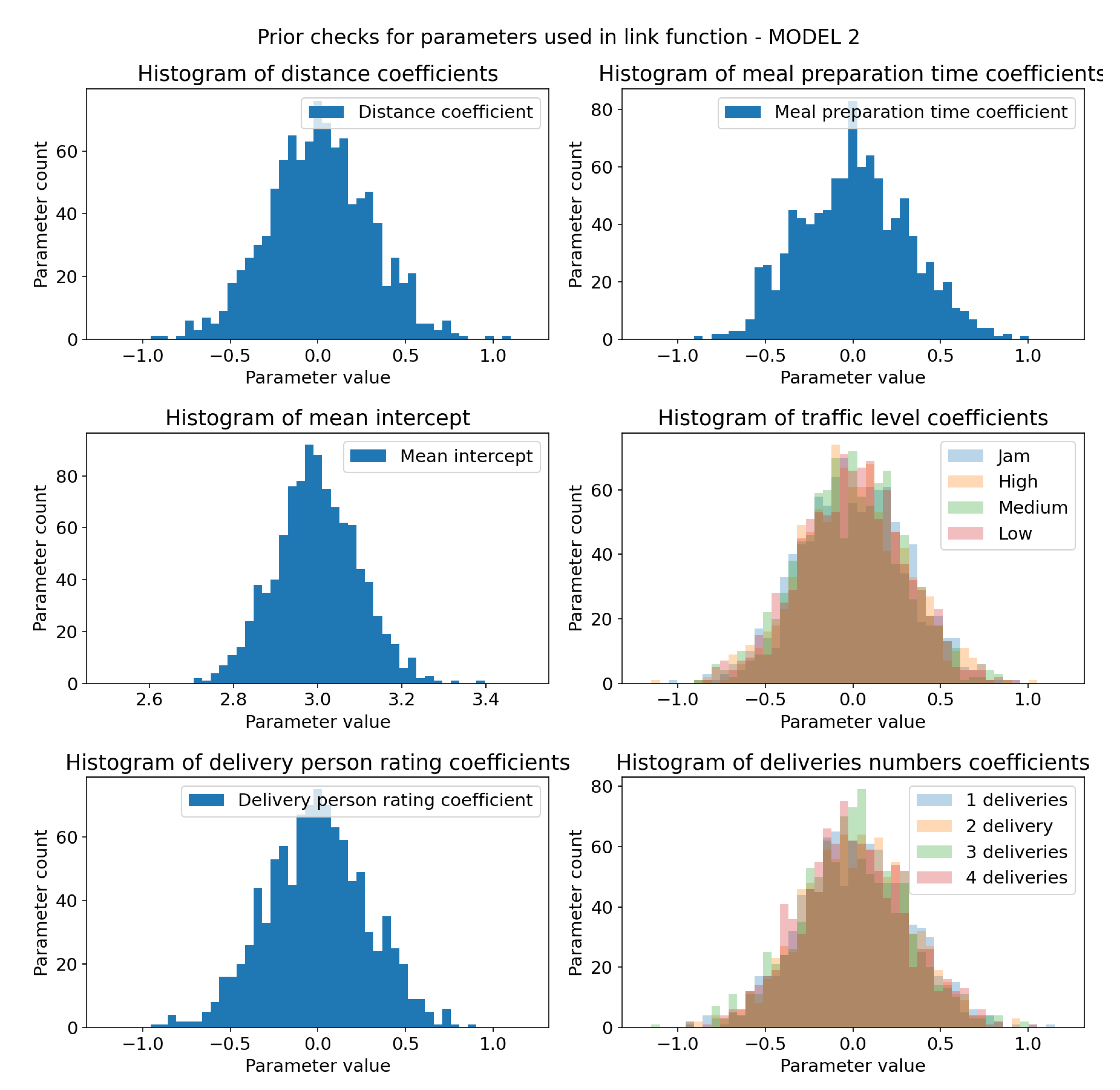
Sampling check for prior distributions of model 2 link function parameters (parameters with _coeff suffix). X-axis represents coefficients values and Y-axis represents sample count. Each of the coefficients follows its distribution, which is necessary for prior check to be successful. (a) Prior distribution of distance coefficient, defined as . (b) Prior distribution of meal preparation time coefficient, defined as . (c) Prior distribution of parameter, defined as . parameter represents our belief of what mean delivery time should be in case all other parameters are 0. (d) Joint plot of prior distributions of traffic level coefficients, all defined as . (e) Prior distribution of delivery person rating coefficient, defined as . (f) Joint plot of prior distributions of deliveries number coefficients, all defined as .
Figure 6.
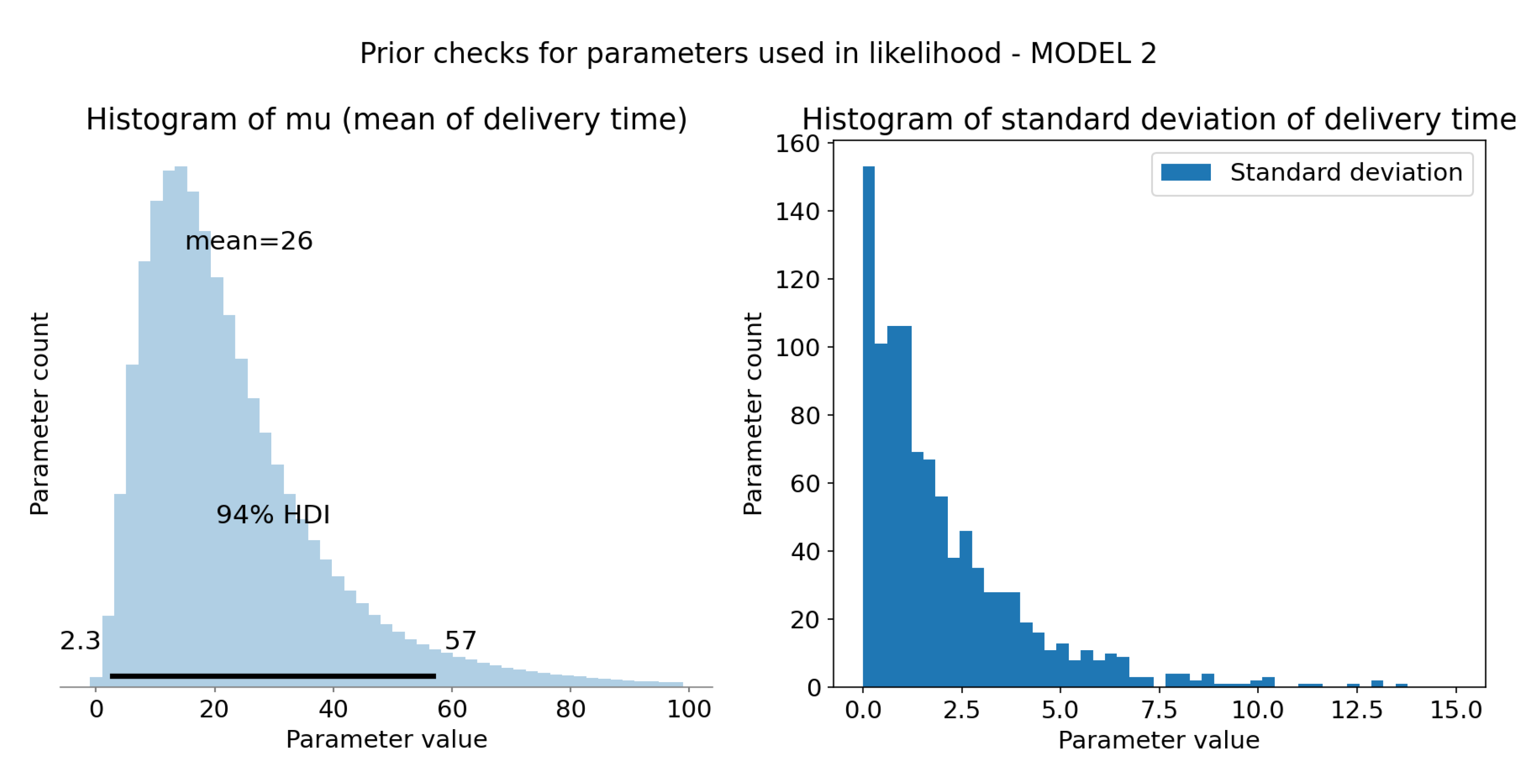
Computation and sample check of model 2 likelihood parameters. X-axis is time in minutes and Y-axis is sample count. (a) Computed represent mean delivery time for each sample. HDI 94% is represented as black bar at the bottom of the plot and tells us that 94% of shown mean times falls in range 2.3 to 57 minutes. Mean of this distribution (at the top of the plot) is 26 minutes, more than for model 1, but still within reasonable range. (b) Prior distribution of standard deviation of the model, defined as .
Figure 7.
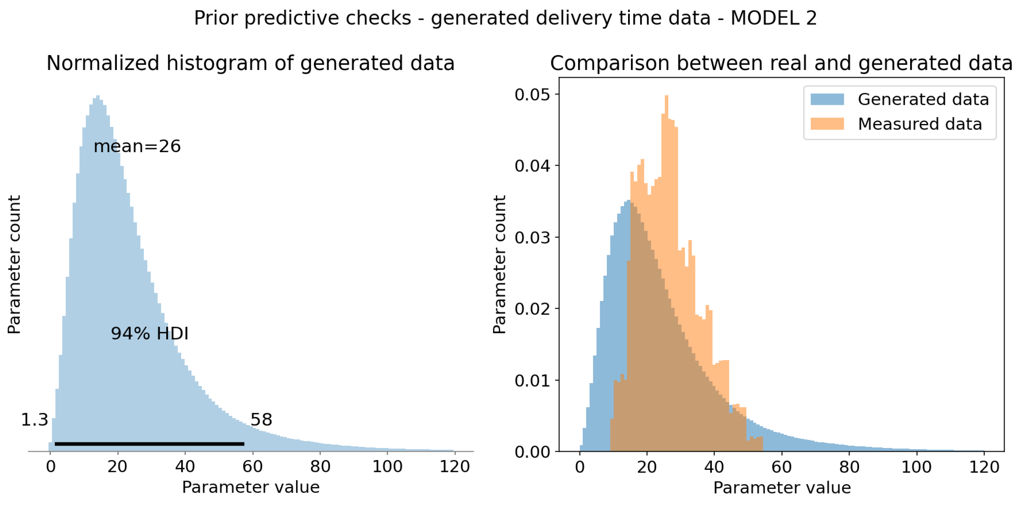
Prior predictive checks - model 2. (a) HDI 94% is represented as black bar at the bottom of the plot and tells us that 94% of shown mean times falls in range 1.3 to 58 minutes. It is very broad, improbable range, but for prior checks it is sufficient. Mean of this distribution (at the top of the plot) is 26 minutes, which is reasonable value. (b) Real and simulated data overlay. Both are normalized, so that integral of the graph is 1. It was necessary for comparison. Measured data is included within generated data, which means that all observations are possible within prior model. This means that prior checks are successful.
3.4.3. Priors and Prior Predictive Checks
We have decided to use unbounded weakly informative priors for all parameters for two main reasons. First, we lack expert knowledge on the influence of each feature. Second, the abundance of data reduces the influence of priors on the final distribution as more data points are added.
We chose a normal distribution with a mean of 0 and a standard deviation of 0.3 for our parameters. This distribution provides a value range of approximately -1 to 1, with most values likely clustering around 0. This choice reflects our initial assumption that each parameter is not highly influential, while still allowing for a small probability that they could be significantly influential. The standard deviation of 0.3 was selected to accommodate the exponential coming from inverse link function, as larger values from the linear combination could numerically destabilize the model.
The exception to this is the intercept parameter, , for which we chose a strong prior: . It results in the base mean delivery time around 15-30 minutes. We opted for a strong prior here to ensure that our model accurately reflects the most average delivery time. Given that our features are standardized with a mean of 0, the linear combination for the most average case would be close to zero, leading to an unrealistic delivery time in the posterior distribution. The prior helps anchor the model, providing a trusted average time for an average case.
For both models prior predictive checks gave good results i.e. observed data was included within simulated data range and no outright impossible values was generated from either of the models.
4. Results
In this section we present posterior distributions of our models. Each one was trained on full data. There was 1000 warm-up and 1000 sampling iterations done on 4 parallel chains. The selected algorithm was Hamiltonian Monte Carlo with engine No-U-Turn Sampler.
4.1. Posterior Predictive Checks for Model 1
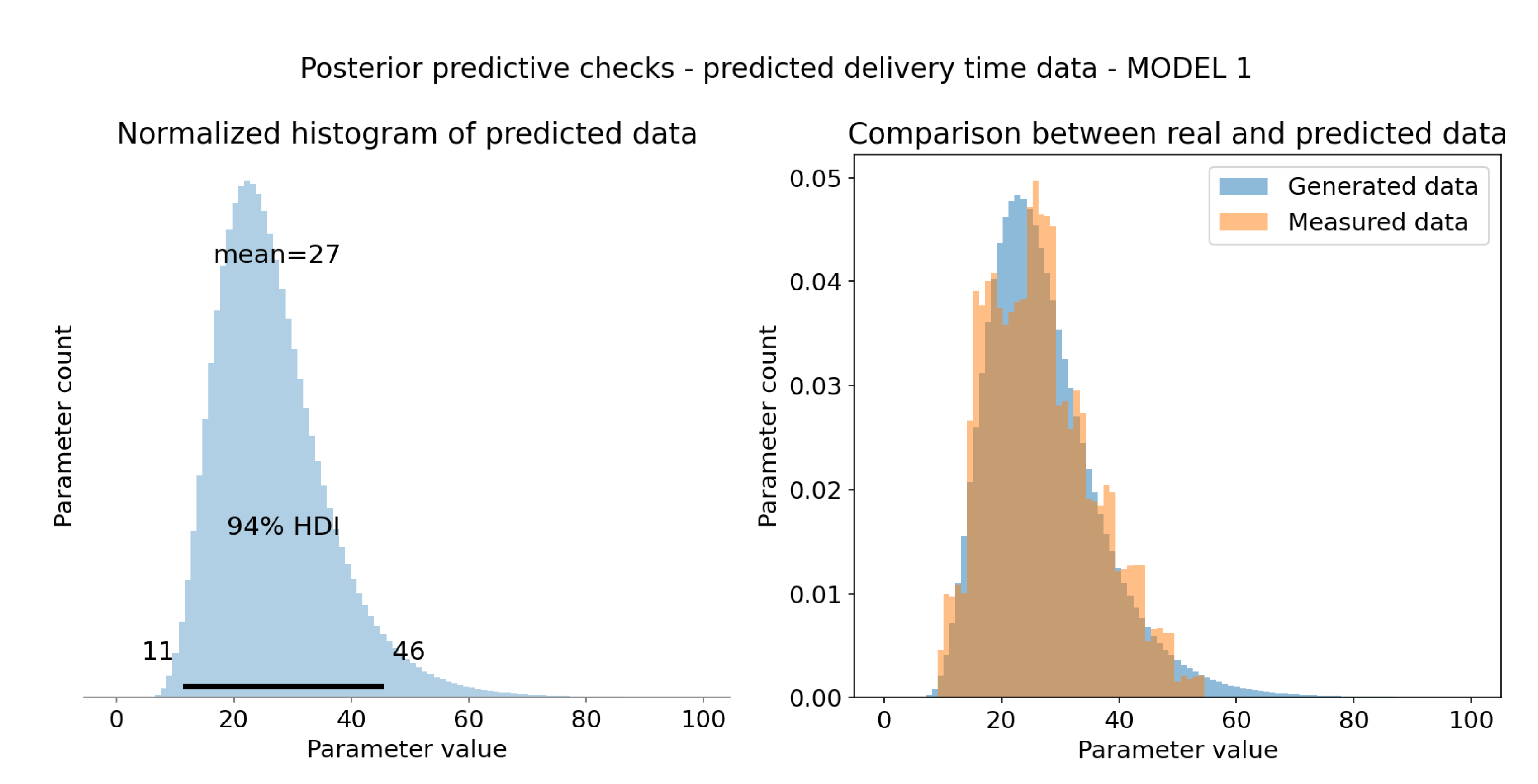
Model 1 gave decent results. All of the observed data falls withing samples from posterior distribution, visual overlap is quite high. Posterior distribution exhibits long tail, which is drawback of using inverse gamma function. Data represented on
Figure 10
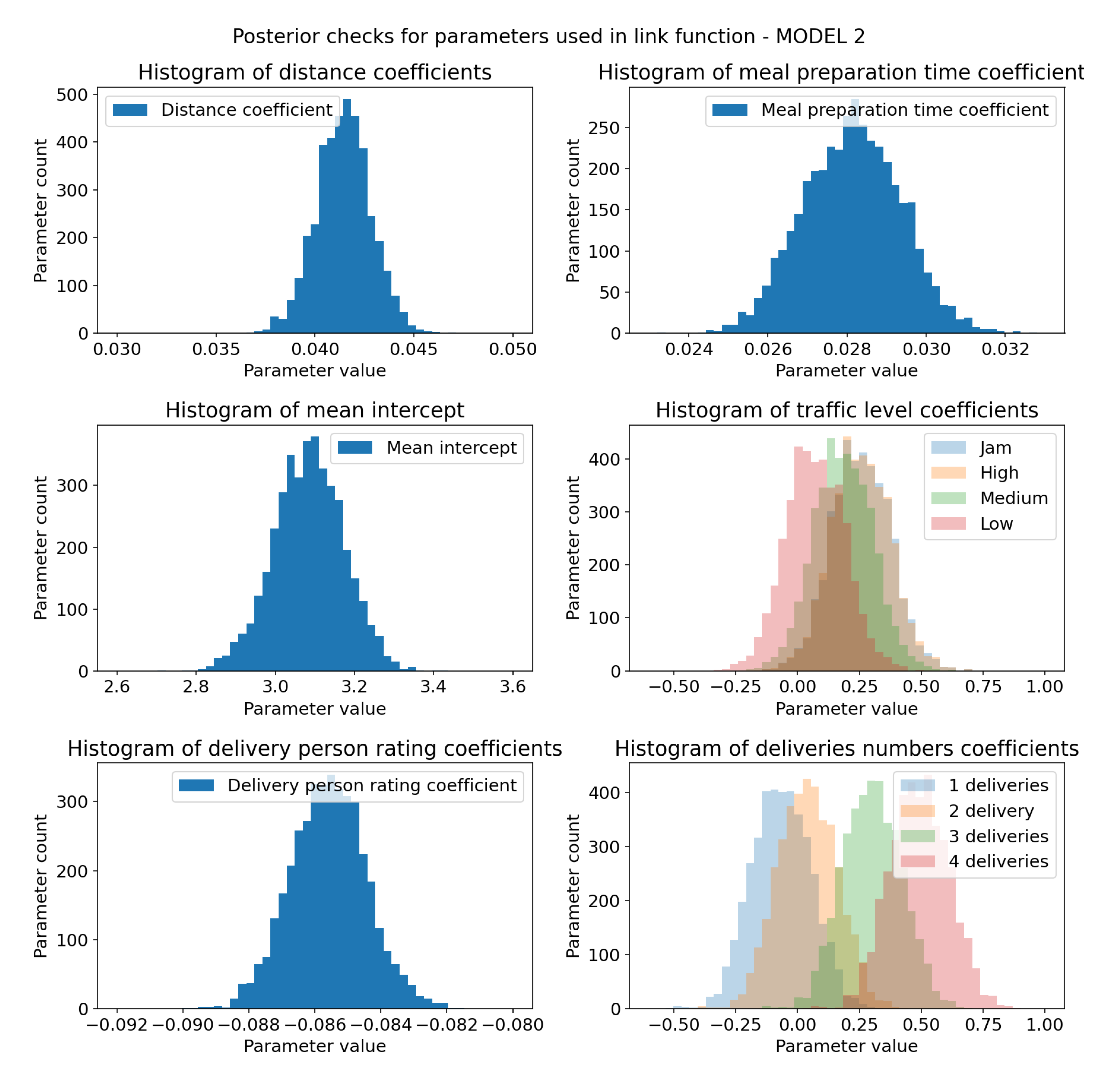
Model coefficients for distance and meal preparation time ended with very narrow distributions, albeit positive ones, indicating that they impact output variable. Mean intercept parameter ended with mean closer to 3.1, which is also closer to the mean of the dataset (
while mean of dataset is
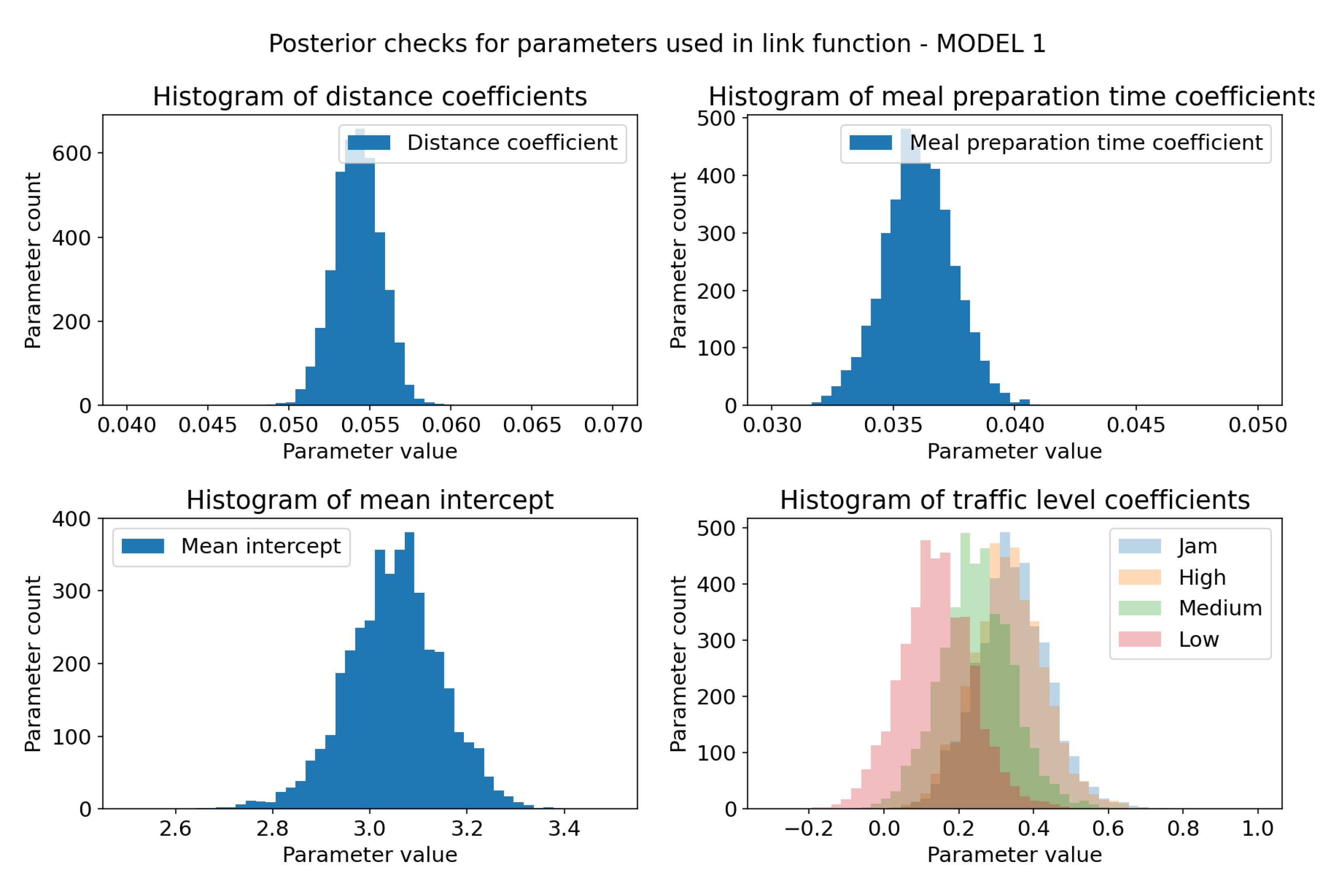
). Traffic level coefficient represent trend, in which low traffic contributes to faster delivery times, and as traffic level increases the delivery times become longer. This interpretation is viable as it is not multiplicand, but sum component, so negative values will result in smaller mean and positive in larger mean. There is almost no distinction between influence of high traffic and jam. Data represented on
Figure 8.
Linear model of mean delivery times
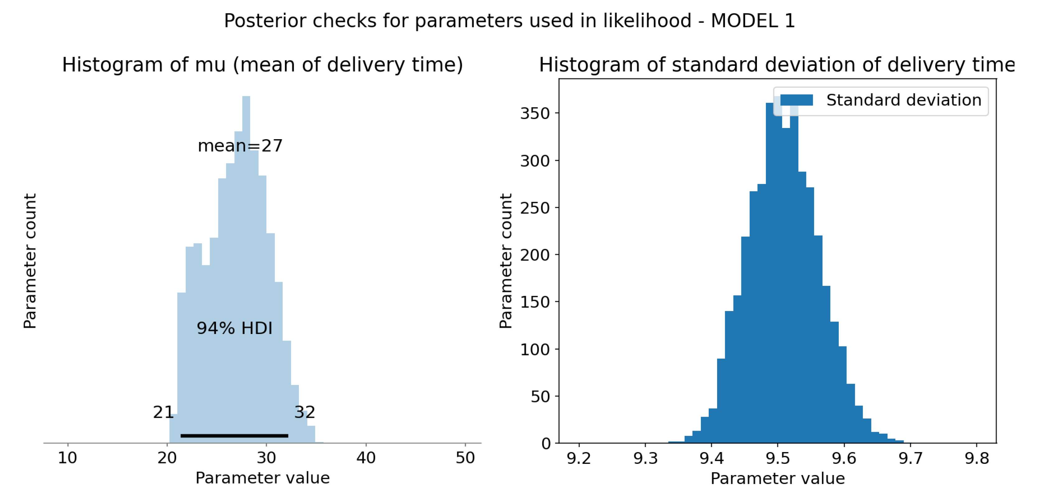
results in probable values with respect to dataset. Standard deviation has completely changed it’s distribution and now follows normal distribution centered around 9.5. It is quite close to std of dataset, which is
. Data represented on
Figure 9.
Figure 8.
Sampling check for posterior distributions of model 1 link function parameters. X-axis represents coefficients values and Y-axis represents sample count. (a) Posterior distribution of distance coefficient. It is much narrower than prior distribution, but still follows normal distribution. Positive value indicates that it has impact on the output variable. (b) Posterior distribution of meal preparation time coefficient. Conclusions the same as for the distance coefficient. (c) Posterior distribution of parameter. It has mean closer to 3.1 which more likely represents mean of the dataset. (d) Joint plot of posterior distributions of traffic level coefficients. The bigger the traffic level, the more impact it has on the outcome variable. Jam and High levels have the same impact.
Figure 9.
Computation and sample check of model 1 likelihood parameters. X-axis represents coefficients values and Y-axis represents sample count.(a) Computed represent mean delivery time for each sample. HDI 94% is represented as black bar at the bottom of the plot and tells us that 94% of shown mean times falls in range 21 to 32 minutes. Those are much more realistic values than the ones from prior distribution. Mean of this distribution (at the top of the plot) is 27 minutes, a reasonable value. (b) Posterior distribution of standard deviation of the model, it no longer resembles prior, now it follows normal distribution with mean ≈ 9.5.
Figure 10.
Posterior predictive checks - model 1. (a) HDI 94% is represented as black bar at the bottom of the plot and tells us that 94% of shown mean times falls in range 11 to 46 minutes. It is broad range, but realistic nevertheless. Mean of this distribution (at the top of the plot) is 27 minutes, which is reasonable value. It follows inverse gamma distribution as defined. (b) Real and simulated data overlay. Both are normalized, so that integral of the graph is 1. It was necessary for comparison. Measured data has high overlap with sampled data from posterior distribution.
4.2. Posterior Predictive Checks for Model 2
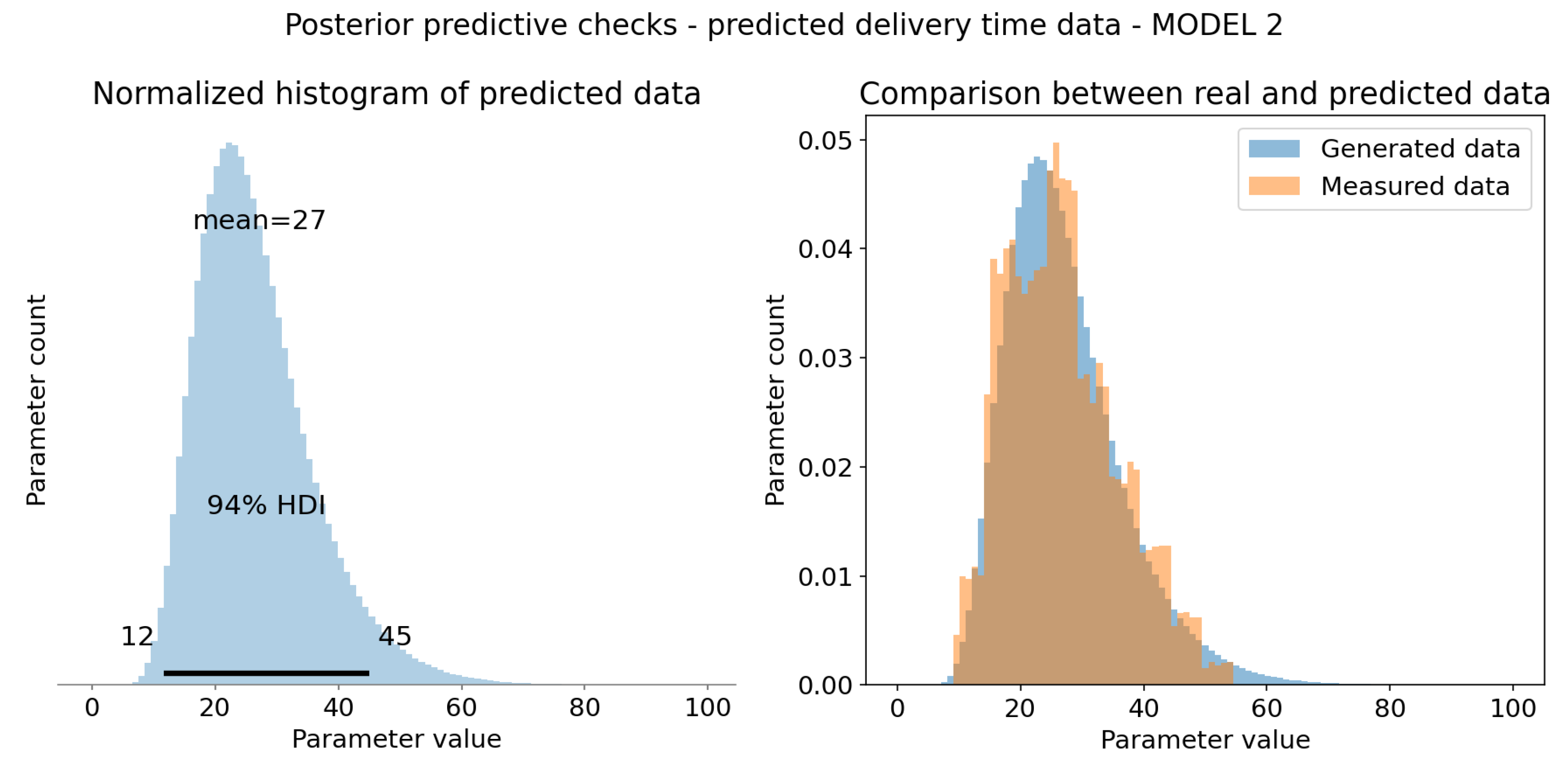
Model 2 gave visually better results. All of the observed data falls withing samples from posterior distribution, as with model 1. Tail is shorter than in Model 1. Data represented on
Figure 12. Since there is not much difference between posterior distributions for shared features of both models, we will only comment on new features, distinct to Model 2, as well as on likelihood related parameters.
Delivery person rating follows narrow normal distribution centered around -0.085. Since it is negative and has small std we can reason that delivery person rating is inversely related to delivery time. This is expected as couriers with higher scores are more likely to deliver food faster. Number of deliveries follows exactly the same trend as traffic level coefficients, but numerically is more important as the values range is greater. Data represented on
Figure 11.
Linear model of mean delivery times
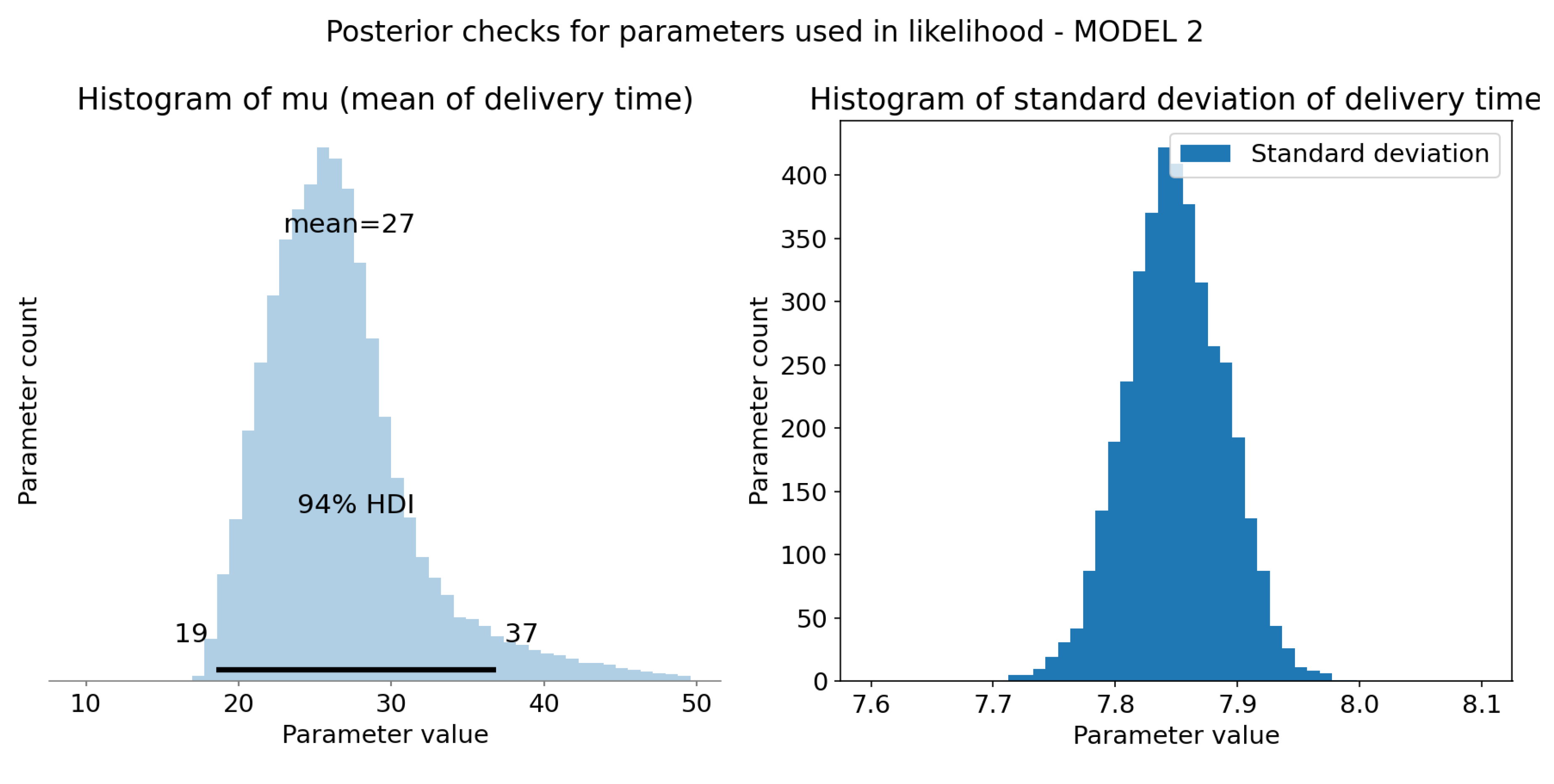
has much longer tail with regards to Model 1, which results in different 94% HDI. Standard deviation has similar distribution to Model 1, although it’s mean value is smaller, around 7.85. Data represented on
Figure 12.
Figure 11.
Sampling check for posterior distributions of model 2 link function parameters. X-axis represents coefficients values and Y-axis represents sample count. (a) Posterior distribution of distance coefficient. It is much narrower than prior distribution, but still follows normal distribution. Positive value indicates that it has impact on the output variable. (b) Posterior distribution of meal preparation time coefficient. Conclusions the same as for the distance coefficient. (c) Posterior distribution of parameter. It has mean closer to 3.1 which more likely represents mean of the dataset. (d) Joint plot of posterior distributions of traffic level coefficients. The bigger the traffic level, the more impact it has on the outcome variable. Jam and High levels have the same impact.(e) Posterior distribution of delivery person rating coefficient. It is much narrower than prior distribution, but still follows normal distribution. Negative values indicate inverse relationship between delivery time and rating; the bigger the courier rating the faster delivery will be made. (f) Joint plot of posterior distributions of deliveries number coefficients. The more deliveries, the more impact it has on the outcome variable. This is the same trend as for traffic level, but greater range translates to greater impact.

Figure 12.
Computation and sample check of model 2 likelihood parameters. X-axis represents coefficients values and Y-axis represents sample count.(a) Computed represent mean delivery time for each sample. HDI 94% is represented as black bar at the bottom of the plot and tells us that 94% of shown mean times falls in range 19 to 37 minutes. Those are much more realistic values than the ones from prior distribution. Mean of this distribution (at the top of the plot) is 27 minutes, a reasonable value. (b) Posterior distribution of standard deviation of the model, it no longer resembles prior, now it follows normal distribution with mean ≈ 7.85.
Figure 13.
Posterior predictive checks - model 2. (a) HDI 94% is represented as black bar at the bottom of the plot and tells us that 94% of shown mean times falls in range 12 to 45 minutes. It is slightly narrower than model 1 range, but realistic nevertheless. Mean of this distribution (at the top of the plot) is 27 minutes, which is reasonable value. It follows inverse gamma distribution as defined. (b) Real and simulated data overlay. Both are normalized, so that integral of the graph is 1. It was necessary for comparison. Measured data has high overlap with sampled data from posterior distribution. Generated data has shorter tail than model 1, which is desirable.
4.3. Models Comparison
Models were compared using WAIC and PSIS-LOO criteria using ArviZ library for exploratory analysis of Bayesian Models [
19].
The WAIC (Widely Applicable or Watanabe-Akaike Information Criterion) is a statistical measure used to estimate the out-of-sample predictive accuracy of a model. It does this by evaluating the within-sample predictive accuracy and making necessary adjustments. WAIC calculates the log pointwise posterior predictive density (LPPD) and includes a correction for the effective number of parameters to account for overfitting. This correction is done by subtracting the sum of the posterior variances of the log predictive densities for each data point [
20].
Table 2.
Comparison result with WAIC criterion.
Table 2.
Comparison result with WAIC criterion.
| Model |
Rank |
waic |
p_waic |
d_waic |
weight |
SE |
dSE |
| 2 |
0 |
-117249.732164 |
14.307179 |
0.000000 |
0.997408 |
145.013769 |
0.000000 |
| 1 |
1 |
-122442.256308 |
9.314501 |
5192.524145 |
0.002592 |
137.412164 |
88.510163 |
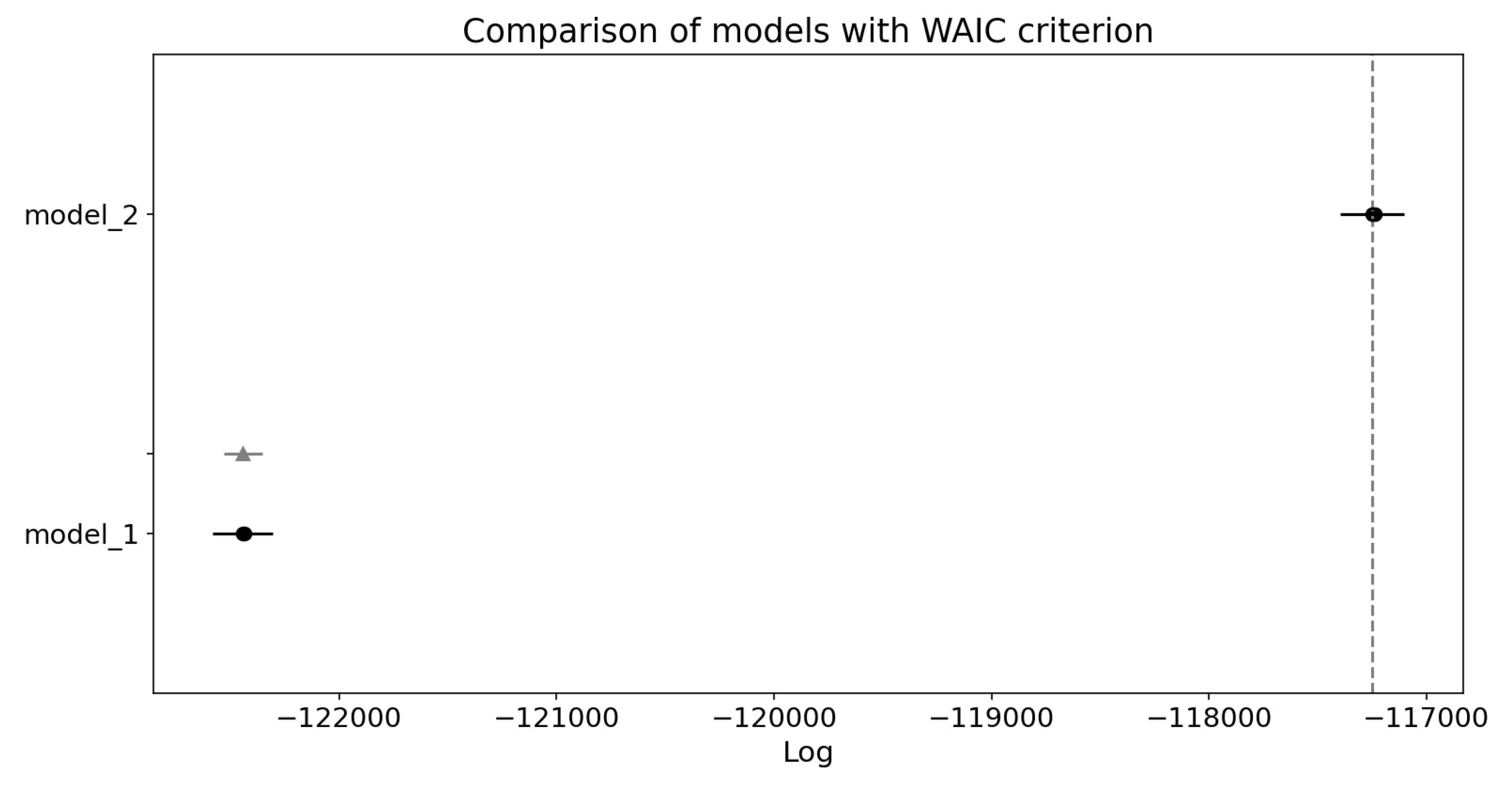
Model 2 has higher ELPD score (denoted as waic) which indicates it’s better within-sample fit. WAIC also correctly states that it has higher number of effective parameters (p_waic). Weight parameter clearly states that Model 2 has near 1 probability within given data. It is slightly more uncertain than Model 1, which is indicated by SE (standard error) parameter, but when compared to differences in WAIC score and size of the dataset, it is not overly large. Overall WAIC clearly evaluated Model 2 as superior.
Figure 14.
Comparison plot for WAIC criterion. Black dots indicate ELPD of each model with their standard error (black lines). Grey triangle represents standard error of difference in ELPD between Model 1 and top-ranked Model 2. Plot indicates that Model 2 performs better.
Figure 14.
Comparison plot for WAIC criterion. Black dots indicate ELPD of each model with their standard error (black lines). Grey triangle represents standard error of difference in ELPD between Model 1 and top-ranked Model 2. Plot indicates that Model 2 performs better.
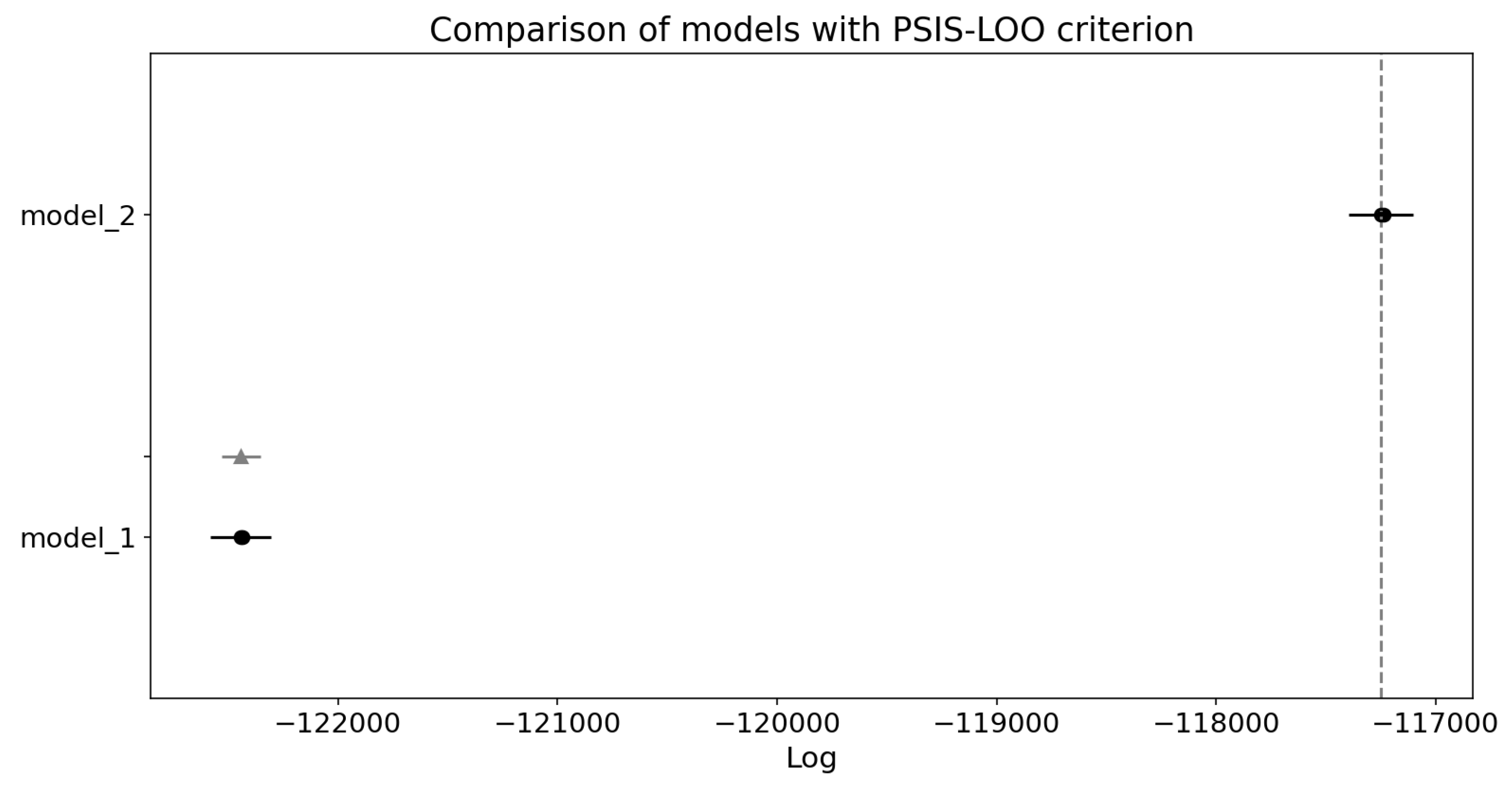
Figure 15.
Comparison plot for PSIS-LOO criterion. Black dots indicate ELPD of each model with their standard error (black lines). Grey triangle represents standard error of difference in ELPD between Model 1 and top-ranked Model 2. Plot indicates that Model 2 performs better.
Figure 15.
Comparison plot for PSIS-LOO criterion. Black dots indicate ELPD of each model with their standard error (black lines). Grey triangle represents standard error of difference in ELPD between Model 1 and top-ranked Model 2. Plot indicates that Model 2 performs better.
The PSIS-LOO (Pareto Smoothed Importance Sampling using Leave-One-Out validation) method is used to calculate out-of-sample predictive fit by summing the log leave-one-out predictive densities. These densities are evaluated using importance ratios (IS-LOO). However, the importance ratios can exhibit high or infinite variance, leading to instability in the estimates. To mitigate this issue, a generalized Pareto distribution is fitted to the largest 20% of the importance ratios [
20].
Table 3.
Comparison result with PSIS-LOO criterion.
Table 3.
Comparison result with PSIS-LOO criterion.
| Model |
Rank |
loo |
p_loo |
d_loo |
weight |
SE |
dSE |
| 2 |
0 |
-117249.732784 |
14.307799 |
0.000000 |
0.997408 |
145.013813 |
0.000000 |
| 1 |
1 |
-122442.256329 |
9.314522 |
5192.523545 |
0.002592 |
137.412164 |
88.510227 |
The PSIS-LOO evaluation provides near identical results as WAIC and the same as above conclusions can be drawn.
5. Conclusions
In this paper, we have explored the application of Bayesian inference for predicting food delivery times, a novel approach not previously employed for this specific task to the best of our knowledge. Our results indicate significant potential in this methodology, particularly with Model 2, which, as an extension of Model 1, demonstrated superior performance. A major advantage of our approach is its ability to capture model uncertainty and provide interpretability, as well as to assess the impact of predictors, thereby offering insights for areas of improvement for food delivery companies. Compared to existing work in this domain, our method presents a novel avenue worthy of further investigation. However, one notable limitation of Bayesian inference is its high computational complexity, which was a challenge in our study as well.
Future research should aim to test these models on data from more reputable sources. This endeavor may prove challenging, as food delivery data is often proprietary and not publicly accessible. Additionally, it is crucial to validate the models with out-of-sample datasets to ensure robustness. Expert input on prior selection should also be considered. Finally, the business applications of these findings merit consideration, both for historical data analysis and real-time implementation.
Author Contributions
Conceptualization, J.P., J.G. and J.B.; methodology, J.P., J.G. and J.B; software, J.P. and J.G.; validation, J.P. and J.B; formal analysis, J.P.; investigation, J.P. ; resources, J.B.; data curation, J.P. and J.G.; writing—original draft preparation, J.P.; writing—review and editing, J.P. and J.B; visualization, J.P.; supervision, J.B.; project administration, J.B; funding acquisition, J.B. All authors have read and agreed to the published version of the manuscript.’
Funding
First author’s work is supported by AGH’s Research University Excellence Initiative under project “Research Education Track”. Third author’s work was partially realised in the scope of project titled ”Process Fault Prediction and Detection”. Project was financed by The National Science Centre on the base of decision no. UMO-2021/41/B/ST7/03851. Part of work was funded by AGH’s Research University Excellence Initiative under project “DUDU - Diagnostyka Uszkodzeń i Degradacji Urządzeń”.
Data Availability Statement
All code prepared as part of this project is available in the repository: https://github.com/JohnnyBeet/Food-delivery-time-prediction/tree/modelling
Conflicts of Interest
The authors declare no conflicts of interest.
Abbreviations
The following abbreviations are used in this manuscript:
| OFD |
Online Food Delivery |
| GPS |
Global Positioning System |
| PSIS-LOO |
Pareto Smoothed Importance Sampling using Leave-One-Out validation |
| WAIC |
Watanabe Akaike Information Criterion |
| DNN |
Deep Neural Network |
| CNN |
Convolutional Neural Network |
| RNN |
Recurrent Neural Network |
| LSTM |
Long-Short Term Memory |
| ETA |
Estimated Time of Arrival |
| OFCT |
Order Fulfilment Cycle Time |
| OD |
Origin-Destination |
| OSRM |
Open Source Routing Machine |
| HDI |
Highest Density Interval |
| LPPD |
Log pointwise Posterior Predictive Density |
| ELPD |
Expected Log pointwise Predictive Density |
| SE |
Standard Error |
| dSE |
Standard Error of the difference between ELPD between each model |
References
- Statista. Online Food Delivery - Worldwide. https://www.statista.com/outlook/emo/online-food-delivery/worldwide, 2024. accessed on 04.05.2024.
- IMARC Group. India Online Food Delivery Market Report. https://www.imarcgroup.com/india-online-food-delivery-market, 2023. accessed on 04.05.2024.
- Alalwan, A.A. Mobile food ordering apps: An empirical study of the factors affecting customer e-satisfaction and continued intention to reuse. International Journal of Information Management 2020, 36, 28–44. [Google Scholar] [CrossRef]
- Abdi, A.; Amrit, C. A review of travel and arrival-time prediction methods on road networks: classification, challenges and opportunities. PeerJ Computer Science 2021, 37, e689. [Google Scholar] [CrossRef] [PubMed]
- Lee, W.H.; Tseng, S.S.; Tsai, S.H. A knowledge based real-time travel time prediction system for urban network. Expert systems with Applications 2009, 36, 4239–4247. [Google Scholar] [CrossRef]
- Li, X.; Cong, G.; Sun, A.; Cheng, Y. Learning travel time distributions with deep generative model. The World Wide Web Conference, 2019, pp. 1017–1027.
- Asghari, M.; Emrich, T.; Demiryurek, U.; Shahabi, C. Probabilistic estimation of link travel times in dynamic road networks. Proceedings of the 23rd SIGSPATIAL International Conference on Advances in Geographic Information Systems, 2015, pp. 1–10.
- Wang, Y.; Zheng, Y.; Xue, Y. Travel time estimation of a path using sparse trajectories. Proceedings of the 20th ACM SIGKDD international conference on Knowledge discovery and data mining, 2014, pp. 25–34.
- Wang, Z.; Fu, K.; Ye, J. Learning to estimate the travel time. Proceedings of the 24th ACM SIGKDD international conference on knowledge discovery & data mining, 2018, pp. 858–866.
- Zhu, L.; Yu, W.; Zhou, K.; Wang, X.; Feng, W.; Wang, P.; Chen, N.; Lee, P. Order fulfillment cycle time estimation for on-demand food delivery. Proceedings of the 26th ACM SIGKDD International Conference on Knowledge Discovery & Data Mining, 2020, pp. 2571–2580.
- Li, Y.; Fu, K.; Wang, Z.; Shahabi, C.; Ye, J.; Liu, Y. Multi-task representation learning for travel time estimation. Proceedings of the 24th ACM SIGKDD international conference on knowledge discovery & data mining, 2018, pp. 1695–1704.
- Wu, C.H.; Ho, J.M.; Lee, D.T. Travel-time prediction with support vector regression. IEEE transactions on intelligent transportation systems 2004, 5, 276–281. [Google Scholar] [CrossRef]
- Wang, H.; Tang, X.; Kuo, Y.H.; Kifer, D.; Li, Z. A simple baseline for travel time estimation using large-scale trip data. ACM Transactions on Intelligent Systems and Technology (TIST) 2019, 10, 1–22. [Google Scholar] [CrossRef]
- Gelman, A.; Carlin, J.B.; Stern, H.S.; Dunson, D.B.; Vehtari, A.; Rubin, D.B. Bayesian Data Analysis, 3rd ed.; Chapman and Hall/CRC: New York, USA, 2013; pp. 1–27. [Google Scholar]
- Team, S.D. Stan Modeling Language Users Guide and Reference Manual, 2.34. https://mc-stan.org/docs/stan-users-guide/index.html. accessed on 13.05.2024.
- Food Delivery Dataset. https://www.kaggle.com/datasets/gauravmalik26/food-delivery-dataset, 2023. accessed on 13.05.2024.
- Gibas, J.; Pomykacz, J.; Baranowski, J. Bayesian modelling of travel times on the example of food delivery: Part 1 - Spatial data analysis and processing. Electronics, 2024. submitted.
- Gelman, A.; Carlin, J.B.; Stern, H.S.; Dunson, D.B.; Vehtari, A.; Rubin, D.B. Bayesian Data Analysis, 3rd ed.; Chapman and Hall/CRC: New York, USA, 2013; pp. 405–411. [Google Scholar]
- ArviZ. API Reference. https://python.arviz.org/en/stable/api/index.html, 2024. accessed on 20.05.2024.
- Vehtari, A.; Gelman, A.; Gabry, J. Practical Bayesian model evaluation using leave-one-out cross-validation and WAIC. Statistics and computing 2017, 27, 1413–1432. [Google Scholar] [CrossRef]
- ArviZ. arviz.compare. https://python.arviz.org/en/stable/api/generated/arviz.compare.html, 2024. accessed on 20.05.2024.
|
Disclaimer/Publisher’s Note: The statements, opinions and data contained in all publications are solely those of the individual author(s) and contributor(s) and not of MDPI and/or the editor(s). MDPI and/or the editor(s) disclaim responsibility for any injury to people or property resulting from any ideas, methods, instructions or products referred to in the content. |
© 2024 by the authors. Licensee MDPI, Basel, Switzerland. This article is an open access article distributed under the terms and conditions of the Creative Commons Attribution (CC BY) license (http://creativecommons.org/licenses/by/4.0/).
