1. Introduction
The e-commerce sector is in a constant state of growth and evolution, particularly within its subdomain of online food delivery (OFD) [
1,
2]. Recent market forecasts indicate a steady rise in revenue for companies offering such services. With numerous players in the market, ensuring customer satisfaction is paramount for a company’s survival. Customers increasingly demand user-friendly applications that simplify the ordering process with just a few taps, while also providing features such as delivery time estimates and communication channels with couriers [
3]. However, estimating delivery times accurately without real-time data presents a significant challenge. While companies can track courier positions via GPS, they lack access to real-time information on factors such as traffic, accidents, and roadworks.
Before any model, algorithm, or computational technique can be applied, the initial step involves finding and preparing data. Effective data analysis and processing play a pivotal role in determining the performance and outcomes of models, given that many techniques rely on clean and comprehensive data. Nonetheless, real-world data seldom meet these ideal conditions and are often challenging to interpret. Even though Bayesian models, which will be explored further in part 2 of this article [
4], are less affected by noisy data and outliers, they still necessitate data processing and sensible assumptions.
Visualization of data is equally significant. It offers valuable insights, particularly when combined with expertise in the relevant field. For instance plotting geospatial data on maps can unveil outliers, patterns, or anomalies. Proper visualization is also essential to draw appropriate conclusion and evaluate models output [
5].
This article leverages spatial data analysis and standard data preprocessing techniques to enhance the data quality utilized in Bayesian models aimed at predicting food delivery times. By examining the spatial distribution of online food deliveries, we identify and rectify faulty data points. Drawing from existing literature, we identify the most crucial features for our models. Additionally, we investigate the relationships between variables in our dataset to uncover any patterns that could impact the behavior of our models.
The contributions of this paper can be summarized as follows: (1) By leveraging the OSRM API, we have effectively transformed raw data into meaningful predictors, which are essential for the implementation of Bayesian models. (2) Standardizing the data proved to be a crucial step for numerical stability in the models without compromising their interpretability. (3) Visualization provided valuable insights into outliers, enabling us to justifiably exclude them from the training data.
The remainder of this paper is organized as follows. In the next section, the relevant studies in the extant literature are reviewed and discussed.
Section 3 provide overview of the used data and describe in details data preprocessing and visualization methods. In
Section 4 we perform in-depth analysis of processing results and spatial analysis of routes. Finally in
Section 5 we make a conclusion and describe the possible future work.
2. Literature Review
Typically OFD platforms acquire customers’ GPS coordinates while their open the app to perform the order [
6]. Then it is used for restaurant recommendations and delivery destination. Subsequently customer GPS coordinates can be used to predict travel time in origin-destination based approach. Although it allows for estimating time without knowing the exact route and distance, a significant issue is that the crucial factor is also the time of departure. Moreover most of the research using origin-destination (OD) based methods have focused on other applications such as taxi trip duration [
7].
Our problem demands that we provide customers with accurate waiting times without relying on knowledge of the precise preparation time [
8] or the courier’s departure. Consequently, OD-based models are unsuitable for our needs. Furthermore, Bayesian models cannot accommodate geographic coordinates as input data. Given the above limitations, transforming GPS coordinates into some form of distance is required.
Joshi et al. have articulated a compelling argument advocating for the consideration of road distance over geometric distances like the Haversine distance for accurate delivery time estimation. They contend that relying solely on geometric distances can result in oversimplified representations, potentially leading to unrealistic data inputs into predictive models. Their approach doesn’t entail route generation, but rather involves mapping GPS coordinates onto a road network map of the analyzed area [
9]. Ji et al. adopt a method for estimating travel time that utilizes GPS trajectories aligned with specific road network segments. Their research, however, is tailored towards optimizing the grouping of tasks related to efficient delivery operations [
10].
Alternatively, some researchers have turned to popular routing tools like Google Maps API, Baidu Maps API, and the TOM-TOM API [
11,
12,
13,
14]. Yet, the utilization of these services incurs exorbitant expenses for OFD companies, often surpassing a staggering one million dollars annually [
15]. As a cost-effective solution, exploration into open-source routing services like OSRM (Open-Source Routing Machine) has been initiated [
16].
The primary objective of spatial analysis in OFD is to explore the factors influencing the utilization of these services, particularly in relation to built infrastructure. Typically, densely populated areas are examined [
14,
17] because online food outlets tend to be more prevalent in urban regions [
18].
Spatial analysis of deliveries or journeys is not as common and typically focuses on exploring the connections between distinct regions[
10,
19]. In the realm of region segmentation, researchers often employ two primary methods: the grid-based approach and the road network-based approach. The grid-based method is particularly useful for visualizing smaller areas as this in Wang et al. article [
19]. Road network based approach is claimed to be more informative yet, in densely populated urban areas, this approach may yield excessively small regions, necessitating a merging step prior to further analysis. [
10].
3. Materials and Methods
3.1. Data
In this study, we employed the Food Delivery Dataset, which is presently accessible on Kaggle [
20]. Initially, the dataset was made available by HackerEarth for their machine learning competition. It encompasses more than 45,000 deliveries spanning 21 cities across India. The data spans a concise three-month period, encompassing February through April of 2023. The dataset includes location of restaurant and delivery destination and other nonspatial information such as weather, traffic conditions, time and date the order was placed.
Table 1 provides a comprehensive list of all variables under consideration, along with their respective meanings.
3.2. Routes Generation
While the exact trajectory of the courier remains uncertain and unpredictable, approximating the route is essential for our purposes. This will not only ensure an appropriate level of reality reproduction, but will also allow to detect incorrect data between which it is impossible to make a delivery. To achieve this, we’ve opted to leverage the OSRM API [
21], an open-source routing engine. By constructing tailored queries containing GPS coordinates for both the starting and ending points of the route, we can utilize the API to generate optimal route suggestions [
22]. Furthermore, customization options such as transportation mode (e.g. car) and route type (e.g.) allow for further refinement of our queries. After receiving the routing request, the OSRM API passes it on to the OSRM routing engine, which employs the OpenStreetMap (OSM) [
23] data to produce the optimal route according to the specified parameters. The routing engine considers multiple factors, including road types, speed limits, and turn restrictions, to guarantee an accurate and efficient route. The output of the routing request contains information about the route, including the route geometry, distance, and estimated travel time. If there is an issue processing the request, API will provide an error code (e.g. "InvalidUrl"), which will inform about the reason of the failure.
3.3. Preproessing
Preparing data as model needed is essential part of delivery time estimation.
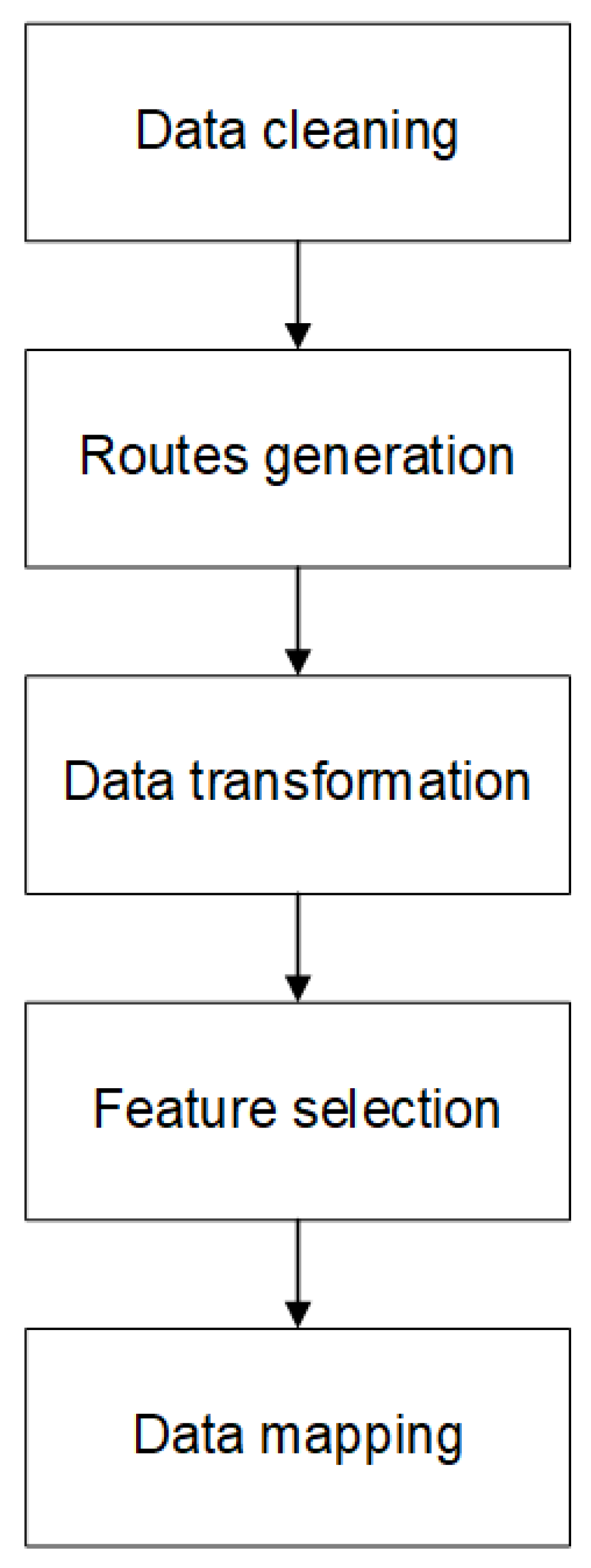
Figure 1 shows preprocessing steps which are described in details in following.
Data cleaning is initial part of preprocessing. It ensures that missig values will not lead to poor results and wrong conclusions. In our approach we decided to remove rows with missing data and rows where restaurant or destination GPS coordinates are outside the India bounding box.
Routes generation is done using OSRM API which was described in
Section 3.2. Created OSRM client uses asynchronous HTTP to find the shortest route between restaurant and delivery destination. If response is successful distance and route geometry are saved, otherwise unsuccessful request and its reason are logged for future analysis. Distance obtained form routing API is integrated with rest of dataset.
Data transformation techniques are used to convert data into sustainable format. Date and time are especially difficult to analyze due to various factors. To overcome this meal preparation time is calculated based on Time_Order and Time_Order_picked. This will enable the model to be utilized in cases where the restaurant furnishes an estimated preparation duration for the order, or where the statistics of preparation time can be derived from historical data [
8].
Feature selection is one of the ways to cope with dimensionality. The goal is to remove irrelevant and redundant features which may include accidental correlations in models and reduce their generalization abilities. Feature selection also decrease the risk of over-fitting and reduce the search space which making learning process faster and less memory consuming [
24].
Feature scaling is a critical step in constructing effective models as it helps mitigate bias stemming from variations in the ranges and magnitudes of data. Among the most widely used techniques are normalization and standardization. We have chosen to implement standardization for selected features with a continuous distribution. This decision ensures that operations and results of the model will be more straightforward to interpret.
Mapping categorical data is essential to use them as input for a model. It’s crucial to note that, unlike in machine learning models, for Bayesian models created using the Stan library [
25], data must be mapped starting from 1 upwards (as vectors are indexed from 1).
3.4. Visualization
As mention previously visualization is also important part of preprocessing. Plotting the data can reveal outliers or anomalies that cannot be easily identify in other ways. In this research we will perform visual analysis of the generated routes followed by analysis of distributions of input data of the models.
The main focus of the route analysis is spatial visualization. We will explore various visualization methods, including heat maps, interactive maps, and road network graph maps. The steps involved in the visualization process are illustrated in Figure.
Figure 1.
For the route analysis, each of the 21 cities is treated separately, allowing for a more detailed examination. The allocation of routes to each city was accomplished through clustering. We utilized the KMeans algorithm provided by scikit-learn [
26], with clustering based on the locations of restaurants and delivery destinations.
To implement interactive maps, we used Folium [
27], which is a wrapper for the Leaflet.js library. Folium allows for the creation of interactive Leaflet maps and supports a wide range of overlay formats, such as images, videos, and GeoJSON, enabling the embedding of multiple layers. For our maps, we used OSM as the base layer and added routes based on the geometry returned by the OSRM API. Additionally, routes from each city were plotted on separate layers for clarity.
Heatmaps are particularly useful for analyzing large datasets or densely located points. Our goal is to depict road usage with an intensity map similar to Navarro’s approach [
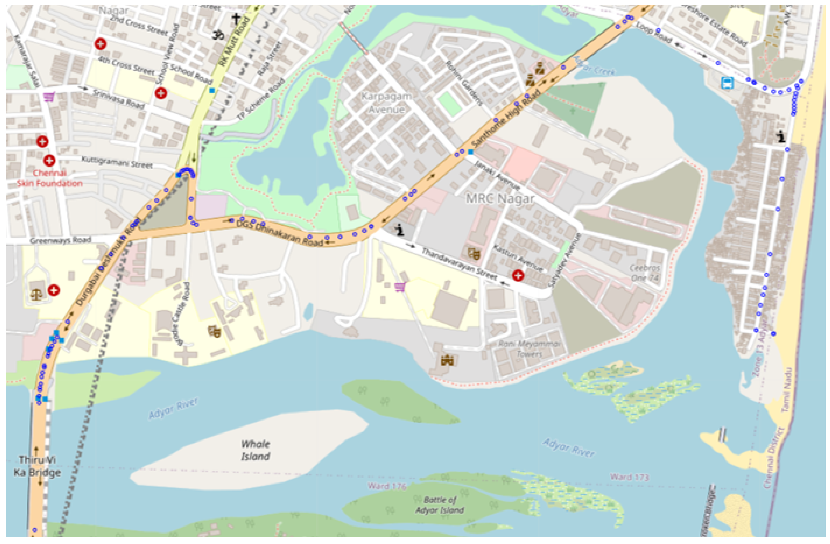
28]. However, the raw route geometry data are unevenly distributed, as illustrated in the
Figure 2. Points are clustered near intersections and turns, whereas on straight sections, the routes are sparsely spaced. To achieve a meaningful scale, we need to interpolate points on these straight sections. We implement linear interpolation for each route segment where the distance between consecutive points exceeds a selected threshold (e.g., 5 meters).
Another method we considered was visualizing routes on road network graphs. This required generating a graph representing the road network. We utilized the OSMnx library [
29], which provides tools to model, analyze, and visualize street networks and other geospatial features from OSM. The generated graph, along with the routes obtained from the OSRM API, needed to be converted into a common format and then plotted as a high-resolution image.
In order to minimize computation time and ensure the appropriate level of map detail we recommend generating a graph only for the city area where the analyzed routes occur. In our case, the maximum and minimum values of longitude and latitude that occurred on routes in a given city were selected as the limit values.
4. Results
4.1. Preprocessing Results
Preprocessing was conducted as outlined in
Section 3.3. During data transformation, we discovered instances where deliveries, from the moment the courier picked up the order to its delivery, were recorded with zero or negative times. Consequently, additional data cleansing was necessary.
To estimate delivery times, companies and researchers commonly utilize a variety of features. These include spatial features (such as the location of the restaurant and destination, and the city road map), cooking time features, order features (like the number of items ordered and the date and time), and courier features (such as workload)[
8,
9,
30,
31,
32]. For our models, we have selected the following variables: the distance between the restaurant and delivery destination, meal preparation time, traffic density, the number of simultaneous deliveries, and courier rating. A detailed analysis of the input data will be presented in
Section 4.1.2.
4.1.1. Routes Generation
All approximate delivery route distances were successfully generated using the OSRM API, with no incorrect routes identified between the restaurant and delivery destination. The histogram of the obtained distances is shown in the accompanying
Figure 3, and the statistics of the road distance projections are presented in the
Table 2. The histogram and statistics reveal that the distances in our dataset are significantly larger than those in other studies. While most deliveries occur within 6 km, as restaurants within this range are shown to customers [
14], our data indicates that the 95th percentile for distance is approximately 28.5 km.
The number of deliveries significantly drops when the distance exceeds 25 km. However, there are routes with distances that are considerably longer. The histogram indicates two distinct groups: one around 65 km and another around 120 km. Both of these groups fall above the 99th percentile, classifying them as outliers. To understand the reasons behind these outliers, we conducted a thorough investigation and compared their routes with other routing engines, particularly Google Maps, which employs different mapping techniques. This comparison will help us identify the causes of these anomalies and develop solutions to prevent such unlikely values in the future.
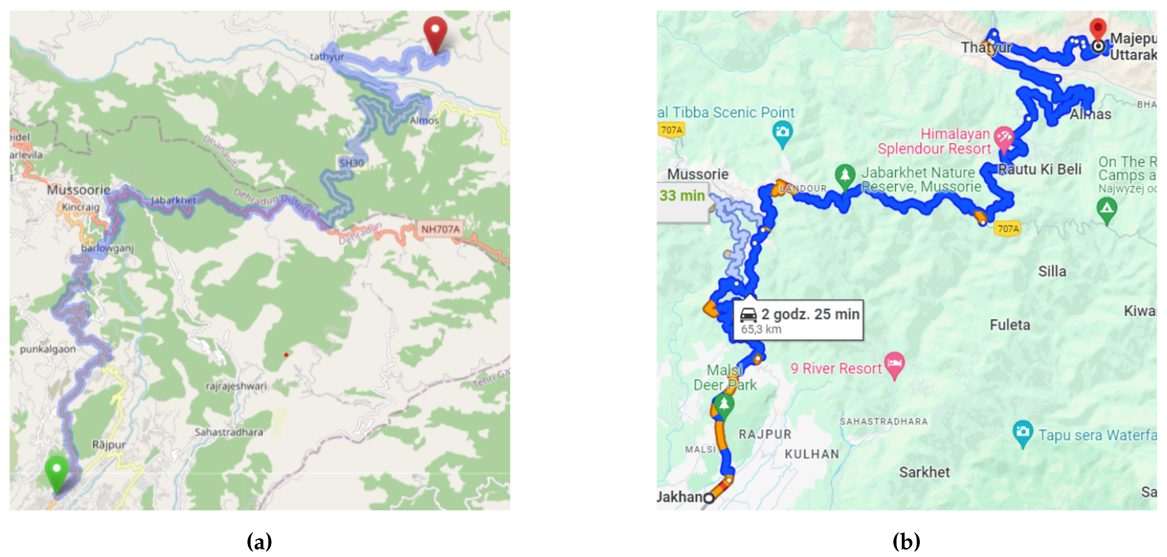
All routes with road distances around 65 km are concentrated in the Dehradun area. Dehradun is situated in a valley at the foot of the Himalayas, resulting in a limited number of roads leading to the surrounding areas. A comparison of the selected route determined by the OSRM API and Google Maps is shown in the
Figure 4. Both engines visually identified the same route; however, Google Maps indicates that the route is approximately 2 km longer. This discrepancy may stem from differences in point positioning on various maps and the distinct distance calculation algorithms used. While the exact route lengths also vary among engines utilizing only OSM data, these differences are negligible over shorter distances.
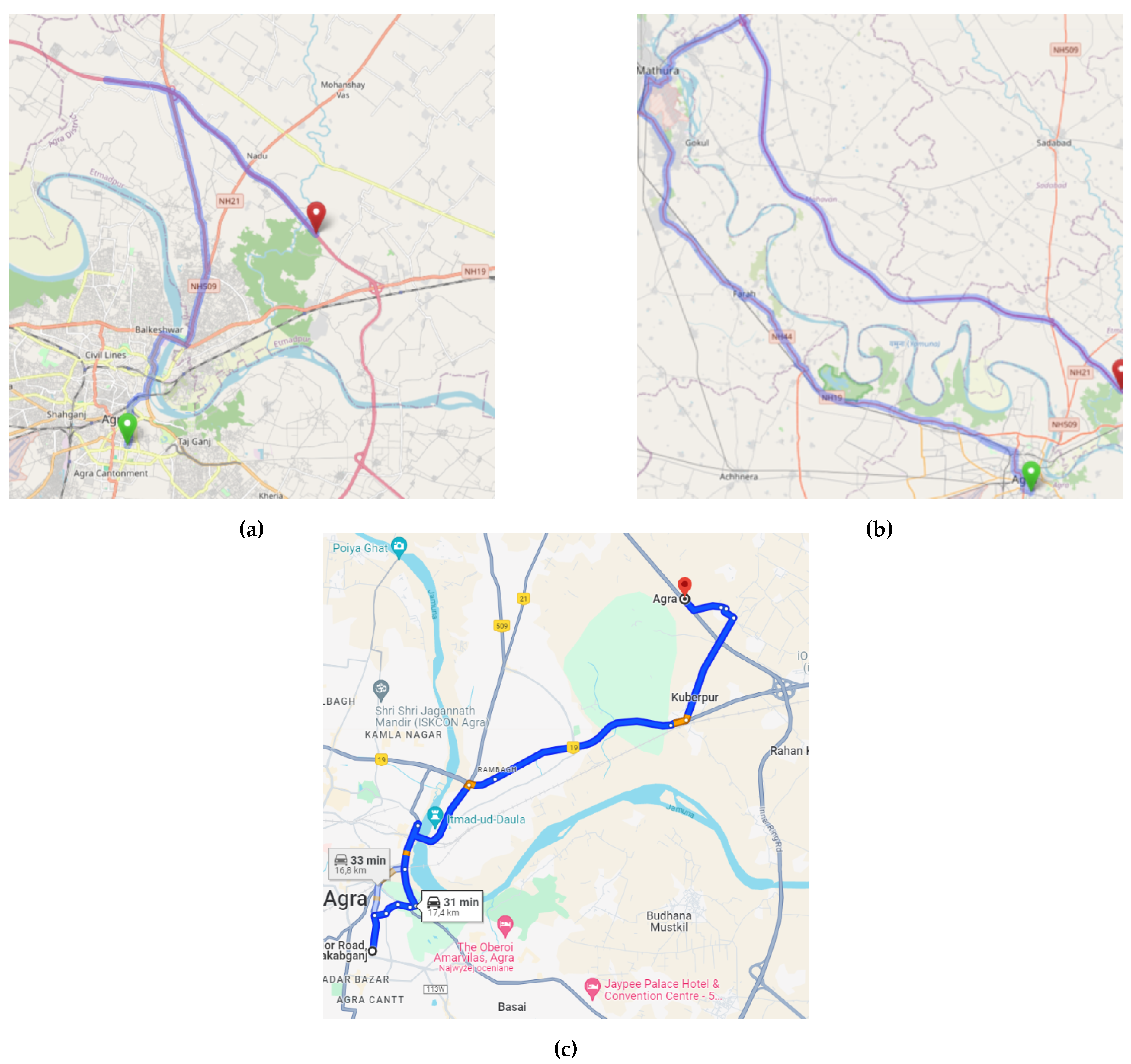
The second problematic group of routes is found in the city of Agra. Analyzing this case is particularly challenging because online routing engines display varying results depending on the day of access. Additionally, Google Maps often selects different destinations for the same location; sometimes directing to an expressway, and other times to a parallel street. The OSM data used by OSRM indicates that the given location is situated in one of the lanes on the nearby Yamuna Expressway. This suggests that the routes allowing direct U-turns on this type of road are incorrectly designated. A comparison of different routes for the same locations is illustrated in the
Figure 5.
To ensure our models are trained on meaningful data, we decided to filter out the outliers. We set a 30 km upper limit for deliveries, which encompasses over 96% of the data available after preprocessing. Standardization was performed after applying this distance filter to prevent excessive data spread caused by biases in the mean and standard deviation.
4.1.2. Input Data Analysis
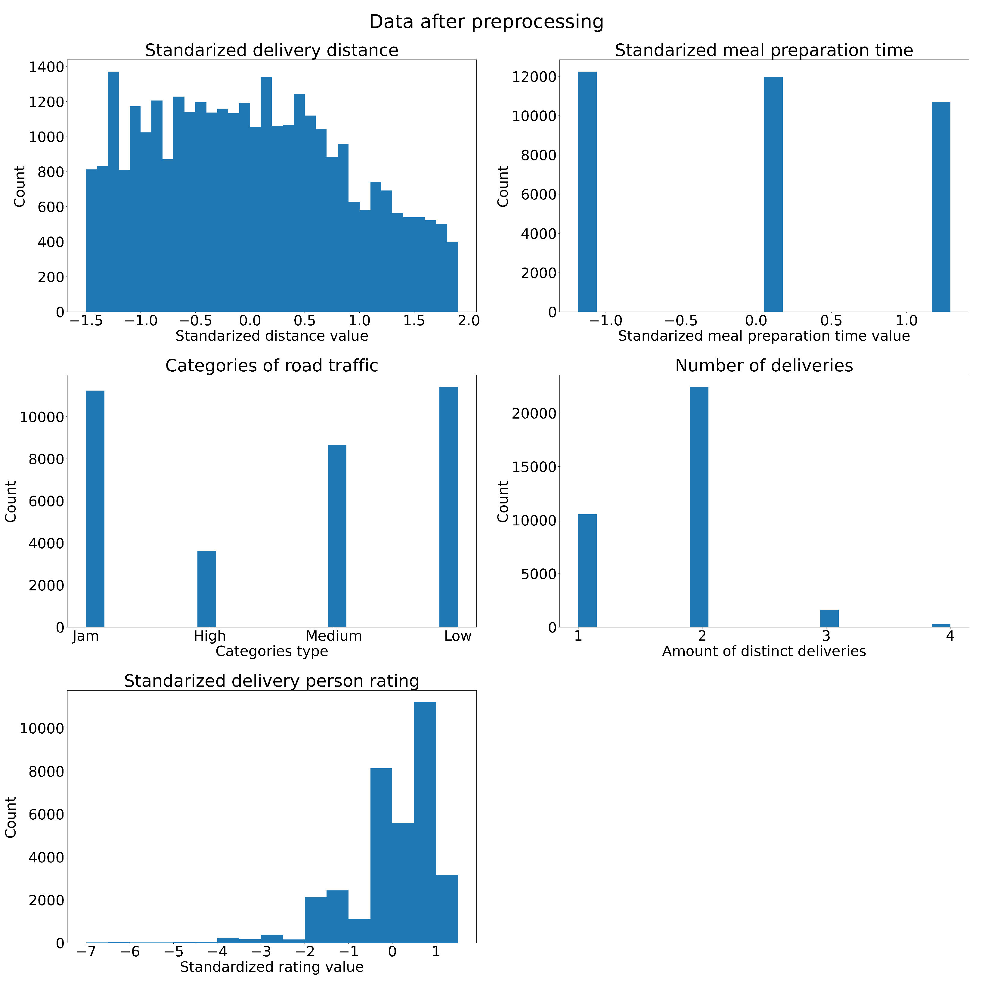
Following the described preprocessing and outlier filtering, we ended up with nearly 35,000 data samples. The data prepared for Bayesian models is presented in the
Figure 6.
The basic distance statistics remained relatively stable after filtration. The average distance decreased to 13.33 km, while the standard deviation reduced to 7.17 km.This outcome was expected, given that the filtered values constituted only about 3% of the dataset eligible for model utilization.
The distribution of order preparation time presents an intriguing puzzle. Initially perceived as a continuous variable, the values are distributed almost evenly across 5, 10, and 15-minute intervals. This phenomenon could stem from the provision of approximate order and pick-up times, rather than precise values.
The prevalence of high ratings among couriers has led to an inflated average of 4.6 in the standardization process. Furthermore, the remarkably small standard deviation of 0.32 translates to substantially reduced standardized values for couriers with lower ratings. Notably, no courier has a rating below 2.5.
The categorical variables "traffic density" and "number of deliveries" appear to align with expectations. Couriers typically handle no more than two deliveries concurrently. Interestingly, deliveries occur with equal frequency during rush hours and periods of very low car traffic. However, deliveries in moderate traffic conditions are relatively less common.
4.2. Spatial Analysis
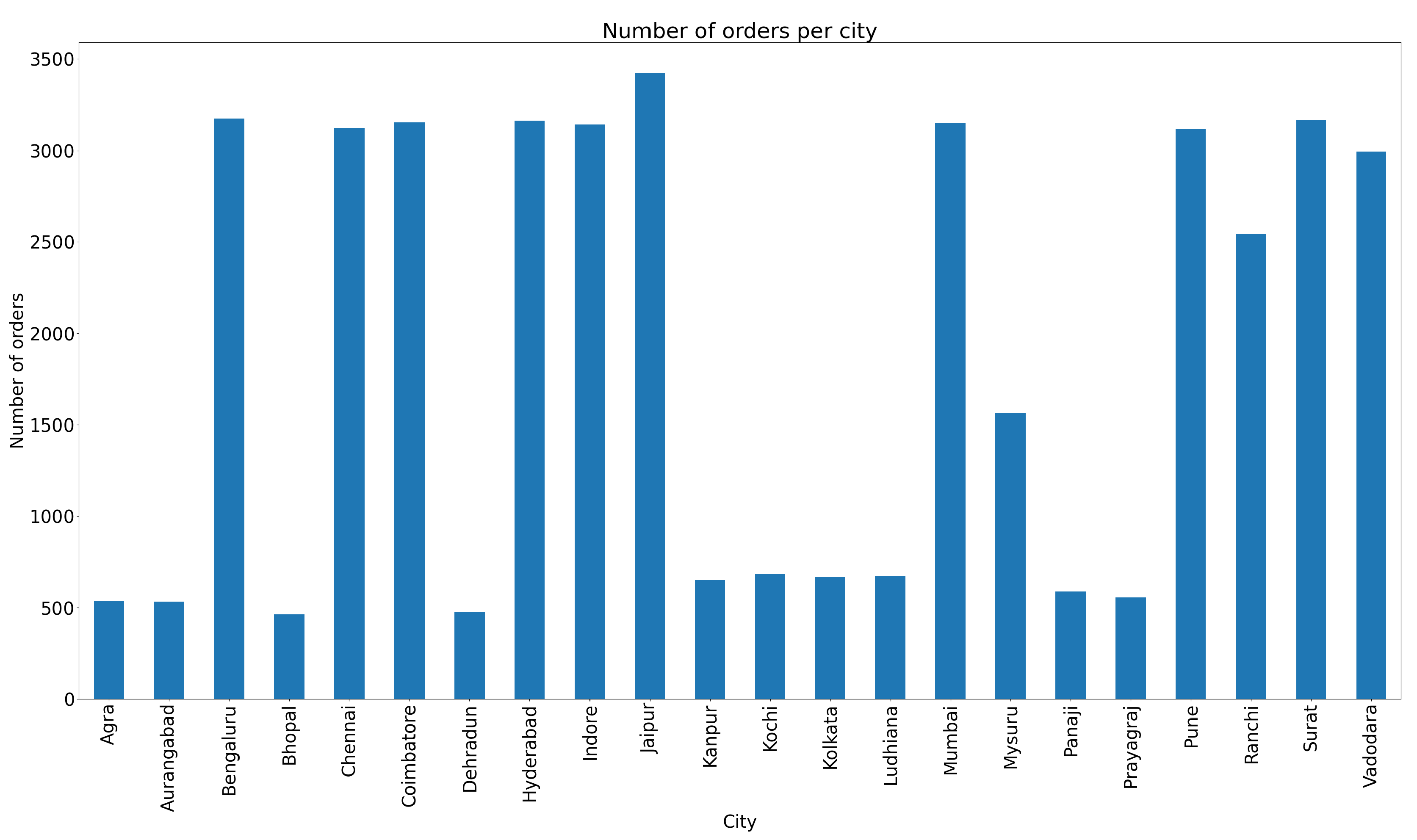
The aim of the spatial analysis was to analyze the frequency of use of road segments. Orders are not evenly distributed among all 21 cities. The analysis included all those located in India and a route for them could be determined (including data considered as outliers). Jaipur is the clear leader in terms of the number of orders, with over 3,400 deliveries located there. eight cities have very similar values at the level of 3,150 deliveries. These include the largest cities in India such as Bangalore and Mumbai. Cities in which the previously calculated outliers occurred have a significantly lower number of deliveries in their area. A chart showing the number of orders for each city is shown in the
Figure 7.
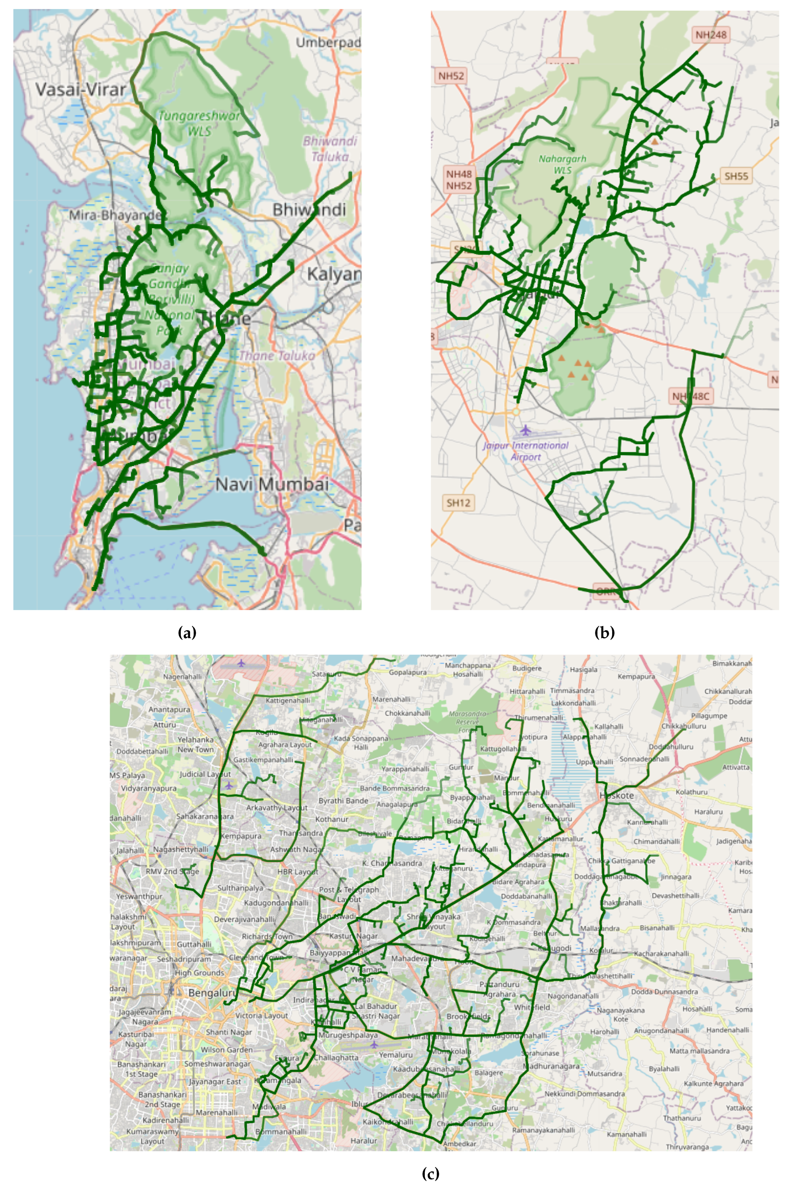
Interactive maps created using Folium present completed routes on a road map with OSM. The intensity of a given road fragment depends on how often it occurs on routes. Additionally, for readability and easier analysis, the routes from each city have been added as a separate layer that can be activated. Sample visualization results are shown in the
Figure 8.
It can be noticed that the roads in city centers are definitely the most intensive. The size of the marker is not related to the results because it is automatically adjusted to the scale. The closer the area, the thinner the drawn routes. Routes that have been traveled once/twice are barely visible, for example this is at the left edge of the Japiur image.
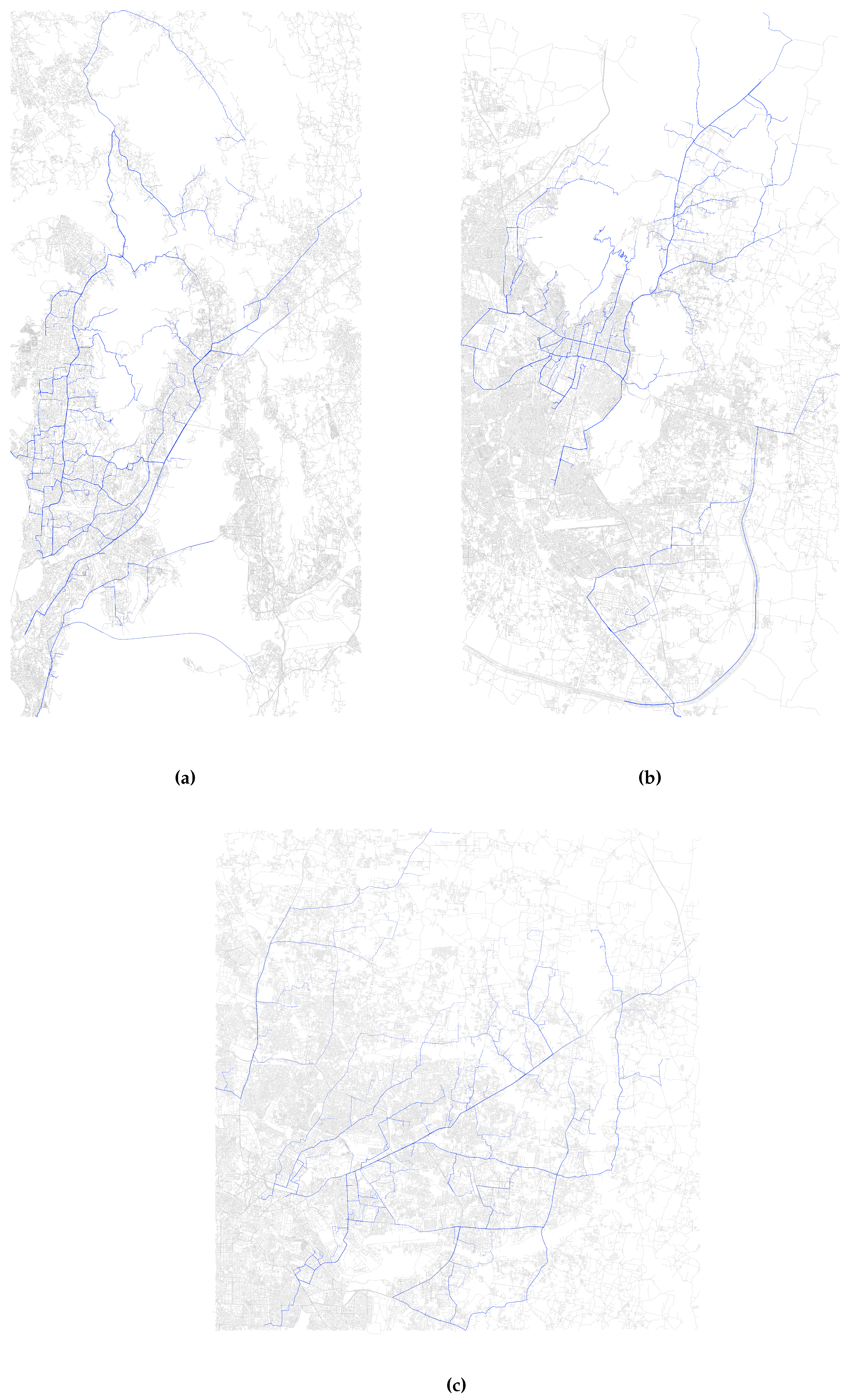
The visualization result using a city graph for similar cities is shown in the
Figure 9. Similarly to the previous maps, the intensity of a road fragment depends on its frequency in the routes. In general in large-scale images generated using OSMnx, differences in saturation levels are not so easily noticeable. Due to the dense network of streets in the centers where deliveries are concentrated, all routes appear to be little traveled. However, after a small zoom they are visible much better than on maps generated using Folium.
The very visible difference in the intensity of bridges on the Mumabiu map made using different methods was interesting, so we decided to analyze it more closely. As it turned out, there was another road running in the immediate vicinity of the bridge, which also had a route which, at a sufficiently large distance, was displayed directly on top of itself, disturbing the results. Moreover, we were dealing with a route that made no sense because it ended in the middle of a bridge (Google maps even projected the point onto the waters of the bay) and it was filtered as outlier (it was about 40 km long)
Despite interpolation to increase the number of points in the routes, heatmap visualization did not bring the expected results. It was not possible to choose such an image scale that, on the one hand, the routes were visible on it, and on the other hand, it was not too large and had some significance. Taking into account that our routes are not concentrated in one area of the city, and there are even two separate clusters of routes (as in the case of Jaipur), our data is not suitable for analysis using a heatmap.
5. Conclusions
This research underscores the importance of data preprocessing and spatial analysis in the context of online food delivery services. By integrating routing information from the OSRM API, we have demonstrated a method for identifying and eliminating outliers in delivery data, thus enhancing the accuracy of subsequent predictive models. Our spatial analyzes indicates that outliers are predominantly deliveries to more distant locations, whereas deliveries within city limits exhibit fewer outliers. This is likely because outliers often stem from incorrect geographic coordinates, which are more apparent in longer-distance deliveries. Therefore, a comprehensive analysis of potential errors in input coordinates is required. It additionally confirms that the OFD market is concentrated in more urbanised areas.
It is important to recognize that this study’s findings may be biased due to the limited amount of data available for each city, which does not accurately reflect the actual workload of OFD companies. Future studies would benefit from obtaining a dataset from one of the leading OFD providers to ensure more comprehensive and representative results.
In the second part of this article, we will delve into the application of Bayesian models to the preprocessed dataset, examining their efficacy in predicting delivery times and exploring potential improvements to the modeling approach. Additionally, future studies could consider refinement of the preprocessing steps, such as advanced handling of missing values and more sophisticated outlier detection methods.
Author Contributions
Conceptualization, J.G., J.P. and J.B.; methodology, J.G., J.P. and J.B; software, J.G. and J.P.; validation, J.G. and J.B; formal analysis, J.G.; investigation, J.G.; resources, J.B.; data curation, J.G. and J.P. ; writing—original draft preparation, J.G.; writing—review and editing, J.G. and J.B; visualization,J.G. and J.P.; supervision, J.B.; project administration, J.B; funding acquisition, J.B. All authors have read and agreed to the published version of the manuscript.’
Funding
Second author’s work is supported by AGH’s Research University Excellence Initiative under project “Research Education Track”. Third author’s work was partially realised in the scope of project titled ”Process Fault Prediction and Detection”. Project was financed by The National Science Centre on the base of decision no. UMO-2021/41/B/ST7/03851. Part of work was funded by AGH’s Research University Excellence Initiative under project “DUDU - Diagnostyka Uszkodzeń i Degradacji Urządzeń”.
Data Availability Statement
Conflicts of Interest
The authors declare no conflicts of interest.
Abbreviations
The following abbreviations are used in this manuscript:
| OFD |
online food delivery |
| GPS |
Global Positioning System |
| OD |
origin-destination |
| OSRM |
Open Source Routing Machine |
| API |
Application Programming Interface |
| OSM |
OpenStreetMap |
References
- Statista. Online Food Delivery - Worldwide. https://www.statista.com/outlook/emo/online-food-delivery/worldwide, 2024. accessed on 04.05.2024.
- IMARC Group. India Online Food Delivery Market Report. https://www.imarcgroup.com/india-online-food-delivery-market, 2023. accessed on 04.05.2024.
- Alalwan, A.A. Mobile food ordering apps: An empirical study of the factors affecting customer e-satisfaction and continued intention to reuse. International Journal of Information Management 2020, 50, 28–44. [Google Scholar] [CrossRef]
- Pomykacz, J.; Gibas, J.; Baranowski, J. Bayesian modelling of travel times on the example of food delivery: Part 2 - Model creation and handling uncertainty. Electronics, 2024; submitted. [Google Scholar]
- Unwin, A. Why is data visualization important? what is important in data visualization? Harvard Data Science Review 2020, 2, 1. [Google Scholar]
- Li, B.; Chen, L.; Xiong, D.; Chen, S.; He, R.; Sun, Z.; Lim, S.; Jiang, H. Simultaneous detection of multiple areas-of-interest using geospatial data from an online food delivery platform (industrial paper). In Proceedings of the Proceedings of the 30th International Conference on Advances in Geographic Information Systems, 2022, pp. 1–10.
- de Araujo, A.C.; Etemad, A. End-to-end prediction of parcel delivery time with deep learning for smart-city applications. IEEE Internet of Things Journal 2021, 8, 17043–17056. [Google Scholar] [CrossRef]
- Zhu, L.; Yu, W.; Zhou, K.; Wang, X.; Feng, W.; Wang, P.; Chen, N.; Lee, P. Order fulfillment cycle time estimation for on-demand food delivery. In Proceedings of the Proceedings of the 26th ACM SIGKDD International Conference on Knowledge Discovery & Data Mining, 2020, pp. 2571–2580.
- Joshi, M.; Singh, A.; Ranu, S.; Bagchi, A.; Karia, P.; Kala, P. Batching and matching for food delivery in dynamic road networks. In Proceedings of the 2021 IEEE 37th international conference on data engineering (ICDE). IEEE; 2021; pp. 2099–2104. [Google Scholar]
- Ji, S.; Zheng, Y.; Wang, Z.; Li, T. Alleviating users’ pain of waiting: Effective task grouping for online-to-offline food delivery services. In Proceedings of the The World Wide Web Conference; 2019; pp. 773–783. [Google Scholar]
- Garus, A.; Christidis, P.; Mourtzouchou, A.; Duboz, L.; Ciuffo, B. Unravelling the last-mile conundrum: A comparative study of autonomous delivery robots, delivery bicycles, and light commercial vehicles in 14 varied European landscapes. Sustainable Cities and Society 2024, 108, 105490. [Google Scholar] [CrossRef]
- Malhotra, I.; Chandra, P.; Majumdar, S.K. Route Optimization Application using Server-Client Architecture and Google APIs. In Proceedings of the 2019 6th International Conference on Computing for Sustainable Global Development (INDIACom). IEEE; 2019; pp. 210–214. [Google Scholar]
- Paithane, P.; Wagh, S.J.; Kakarwal, S. Optimization of route distance using k-NN algorithm for on-demand food delivery. System research and information technologies 2023, 85–101. [Google Scholar]
- Wang, Z.; He, S.Y. Impacts of food accessibility and built environment on on-demand food delivery usage. Transportation Research Part D: Transport and Environment 2021, 100, 103017. [Google Scholar] [CrossRef]
- Yu, X.; Li, X.Y.; Zhao, J.; Shen, G.; Freris, N.M.; Zhang, L. Antigone: Accurate navigation path caching in dynamic road networks leveraging route apis. In Proceedings of the IEEE INFOCOM 2022-IEEE Conference on Computer Communications. IEEE; 2022; pp. 1599–1608. [Google Scholar]
- Fu, J.; Bhatti, H.J.; Eek, M. Optimization of Freight Charging Infrastructure Placement Using Multiday Travel Data. In Proceedings of the 2023 IEEE 26th International Conference on Intelligent Transportation Systems (ITSC). IEEE; 2023; pp. 1576–1582. [Google Scholar]
- Hu, X.; Zhang, G.; Shi, Y.; Yu, P. How Information and Communications Technology Affects the Micro-Location Choices of Stores on On-Demand Food Delivery Platforms: Evidence from Xinjiekou’s Central Business District in Nanjing. ISPRS International Journal of Geo-Information 2024, 13, 44. [Google Scholar] [CrossRef]
- Keeble, M.; Adams, J.; Bishop, T.R.; Burgoine, T. Socioeconomic inequalities in food outlet access through an online food delivery service in England: A cross-sectional descriptive analysis. Applied geography 2021, 133, 102498. [Google Scholar] [CrossRef] [PubMed]
- Wang, L.; Fu, H.; Wu, S.; Liu, Q.; Tan, X.; Huang, F.; Zhang, M.; Wu, W. CAMLO: Cross-Attentive Multi-View Network for Long-Term Origin-Destination Flow Prediction. In Proceedings of the 2024 SIAM International Conference on Data Mining (SDM), SIAM, 2024, pp. 454–462.
- Food Delivery Dataset. https://www.kaggle.com/datasets/gauravmalik26/food-delivery-dataset, 2023. accessed on 13.05.2024.
- Open Source Routing Machine. https://project-osrm.org/, 2024. accessed on 13.05.2024.
- Open Source Routing Machine API. https://project-osrm.org/docs/v5.5.1/api/#route-service, 2024. accessed on 13.05.2024.
- OpenStreetMap. https://www.openstreetmap.org/, 2024. accessed on 13.05.2024.
- García, S.; Ramírez-Gallego, S.; Luengo, J.; Benítez, J.M.; Herrera, F. Big data preprocessing: methods and prospects. Big data analytics 2016, 1, 1–22. [Google Scholar] [CrossRef]
- Stan. https://mc-stan.org/, 2024. accessed on 14.05.2024.
- Pedregosa, F.; Varoquaux, G.; Gramfort, A.; Michel, V.; Thirion, B.; Grisel, O.; Blondel, M.; Prettenhofer, P.; Weiss, R.; Dubourg, V.; et al. Scikit-learn: Machine learning in Python. the Journal of machine Learning research 2011, 12, 2825–2830. [Google Scholar]
- Folium. https://python-visualization.github.io/folium/latest/, 2024. accessed on 14.05.2024.
- Navarro, D. How to Visualise a Billion Rows of Data in R with Apache Arrow. https://blog.djnavarro.net/posts/2022-08-23_visualising-a-billion-rows, 2022. accessed on 15.05.2024.
- Boeing, G. Modeling and Analyzing Urban Networks and Amenities with OSMnx 2024.
- The Swiggy Delivery Challenge. https://bytes.swiggy.com/the-swiggy-delivery-challenge-part-one-6a2abb4f82f6, 2018. accessed on 18.05.2024.
- DeepETA: How Uber Predicts Arrival Times Using Deep Learning. https://www.uber.com/en-PL/blog/deepeta-how-uber-predicts-arrival-times/, 2022. accessed on 18.05.2024.
- Predicting Time to Cook, Arrive, and Deliver at Uber Eats. https://www.infoq.com/articles/uber-eats-time-predictions/, 2019. accessed on 18.05.2024.
Figure 1.
Preprocessing steps include: deletion of incomplete or out-of-India samples, generating routes via OSRM API, converting the date and time into a sustainable format, selecting predictors with the greatest information value and mapping data to format appropriate for Bayesian model.
Figure 1.
Preprocessing steps include: deletion of incomplete or out-of-India samples, generating routes via OSRM API, converting the date and time into a sustainable format, selecting predictors with the greatest information value and mapping data to format appropriate for Bayesian model.
Figure 2.
Raw distribution of sample route geometry. GPS coordinates are clustered near intersections and turns, whereas on straight sections, there are sparsely spaced. Considering raw distribution of routes geometry data for some visualization method interpolation is necessary.
Figure 2.
Raw distribution of sample route geometry. GPS coordinates are clustered near intersections and turns, whereas on straight sections, there are sparsely spaced. Considering raw distribution of routes geometry data for some visualization method interpolation is necessary.
Figure 3.
Histogram of total distance of generated routes, each bin represent 1 km interval. Most of the deliveries have distance under 25 km. Two peaks in the distribution corresponds to distance 2-3km and 4-5km, which indicates orders from restaurants recommended by application. Moreover two outliers group can be identified (around 65 km and 120km).
Figure 4.
Comparison of routes determined using different routing engines. (a) Rout obtained using OSRM on OSM. (b) Route obtained using Google Maps. Both services generate approximately the same route (difference in distance compared to the length of the entire routes negligible).
Figure 4.
Comparison of routes determined using different routing engines. (a) Rout obtained using OSRM on OSM. (b) Route obtained using Google Maps. Both services generate approximately the same route (difference in distance compared to the length of the entire routes negligible).
Figure 5.
Comparison of routes result. (a) Route obtained using OSRM on OSM which involve direct U-turn on Yamuna Expressway (obtained 18.05.2024). (b) Route obtained using OSRM on OSM which (obtained 16.04.2024). (c) Route obtained using Google Maps that map location on road near Yamuna Expressway (obtained 18.05.2024). The lack of repeatability in the obtained routes may result from the lack of a direct point corresponding to the coordinate from the dataset.
Figure 6.
Histograms of data used in inference. (a) Standardized distance, bins defined as <-1.5;2> with step 0.1. (b) Standardized meal preparation time, 20 bins equally spaced, automatically defined by program. (c) Categories of road traffic, from highest to lowest. (d) Distinct deliveries count. (e) Standardized delivery person rating, bins defined as <-7;2> with step 0.5
Figure 7.
Number of orders in each city. Larger Indian cities have a higher number of orders, while in smaller cities there are even 6 times fewer orders. This confirms that ordering food online is a typical urban phenomenon.
Figure 7.
Number of orders in each city. Larger Indian cities have a higher number of orders, while in smaller cities there are even 6 times fewer orders. This confirms that ordering food online is a typical urban phenomenon.
Figure 8.
Routes visualizations using Folium for (a) Mumbai, (b) Jaipur and (c) Bangalore. Sections of roads that were heavily trafficked with deliveries have a more intense color, while sections that have been traveled once or twice are much less visible.
Figure 8.
Routes visualizations using Folium for (a) Mumbai, (b) Jaipur and (c) Bangalore. Sections of roads that were heavily trafficked with deliveries have a more intense color, while sections that have been traveled once or twice are much less visible.
Figure 9.
Routes visualizations of routes on a city street graph made in OSMnx for (a) Mumbai, (b) Jaipur and (c) Bangalore. Sections of roads that were heavily trafficked with deliveries have a more intense color, while sections that have been traveled once or twice are much less visible.
Figure 9.
Routes visualizations of routes on a city street graph made in OSMnx for (a) Mumbai, (b) Jaipur and (c) Bangalore. Sections of roads that were heavily trafficked with deliveries have a more intense color, while sections that have been traveled once or twice are much less visible.
Table 1.
Data description.
Table 1.
Data description.
| Variabel name |
Meaning |
| Restaurant_latitude |
Latitude of the restaurant |
| Restaurant_longitude |
Longitude of the restaurant |
| Delivery_location_latitude |
Latitude of the delivery destination |
| Delivery_location_longitude |
Longitude of the delivery destination |
| Road_traffic_density |
Road traffic intensity (Low, Medium, High or Jam) |
| Weatherconditions |
Current weather conditions (e.g. Sunny, Stormy, Fog ) |
| multiple_deliveries |
Quantity of simultaneous deliveries (number 0-4) |
| Delivery_person_Ratings |
Average rating of the courier |
| Delivery_person_Age |
Age of the courier |
| Order_Date |
Date of placing the order |
| Time_Orderd |
Time of placing the order |
| Time_Order_picked |
Time of picking up by courier |
| Time_taken |
Delivery time in minutes |
Table 2.
Routes statistics.
Table 2.
Routes statistics.
| Total number of routes |
41522 |
| Average route distance |
13.99 km |
| Standard deviation of route distance |
8.42 km |
| Minimum route distance |
1.49 km |
| 95th percentile |
28.53 km |
| 99th percentile |
36.42 km |
| Maximum route distance |
121.89 km |
| ]2*Maximum number of routes in distance interval |
2-3km (2331) |
| |
4-5km (2153) |
|
Disclaimer/Publisher’s Note: The statements, opinions and data contained in all publications are solely those of the individual author(s) and contributor(s) and not of MDPI and/or the editor(s). MDPI and/or the editor(s) disclaim responsibility for any injury to people or property resulting from any ideas, methods, instructions or products referred to in the content. |
© 2024 by the authors. Licensee MDPI, Basel, Switzerland. This article is an open access article distributed under the terms and conditions of the Creative Commons Attribution (CC BY) license (http://creativecommons.org/licenses/by/4.0/).
