Submitted:
20 June 2024
Posted:
21 June 2024
You are already at the latest version
Abstract
Keywords:
1. Introduction
2. Literature Review
3. Dynamic Models and the Controller Design of a Wheeled Mobile Robot
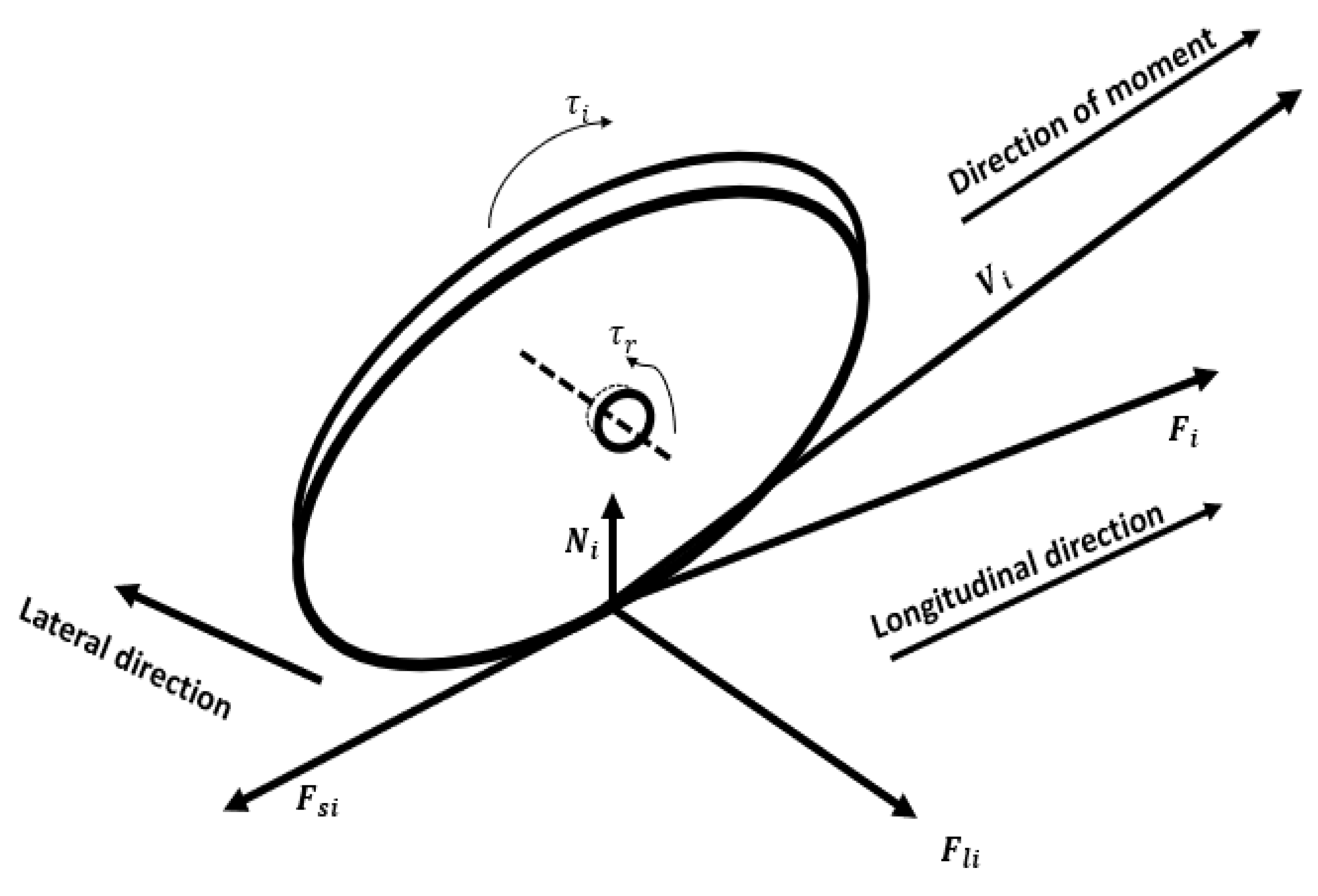
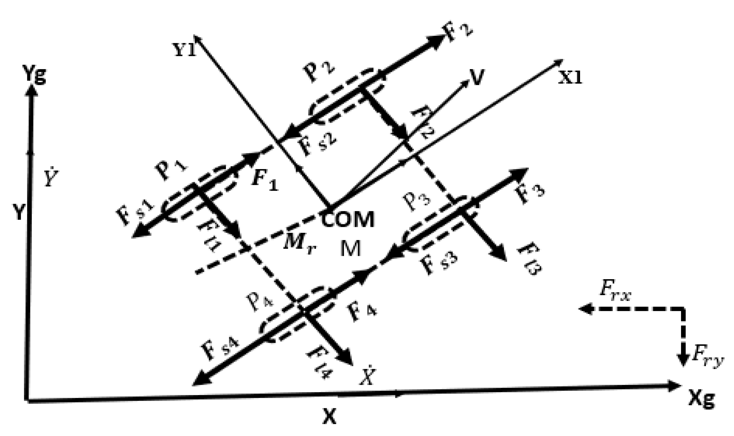
3.1. Development of a Kinematic Model of a Four-Wheeled Mobile Robot for Agricultural Applications
- linearity: assuming that the system behaves in a linear manner, where the output is directly proportional to the input, this simplifies the mathematical analysis and allows for the use of linear techniques
- time-invariance: assuming that the system’s behaviour does not change over time, this means that the system’s properties and characteristics remain constant throughout the modelling period
- homogeneity: assuming that the system’s behaviour is uniform throughout its spatial domain, this means that the system’s properties and characteristics are the same at all points in space
- determinism: assuming that the system’s behaviour is fully determined by its initial conditions and inputs, this excludes the influence of random or stochastic factors
- perfect knowledge: assuming that all relevant information about the system is known and available for modelling purposes, this includes complete knowledge of the system’s structure, parameters and boundary conditions.
3.2. Hybridisation Controller Design for a Wheeled Mobile Robot
- A.
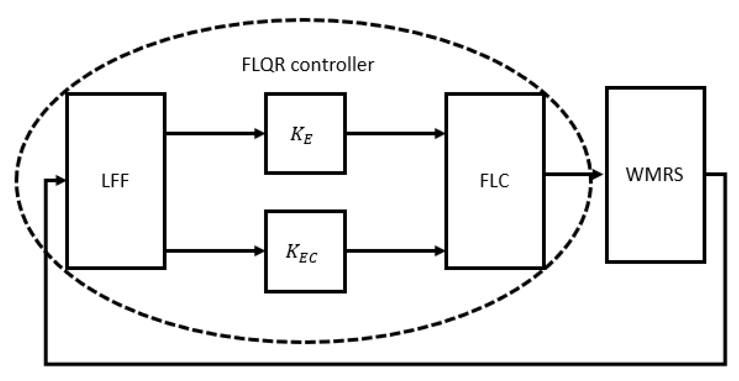
- Fuzzy linear quadratic regulator (FLQR)
- B.
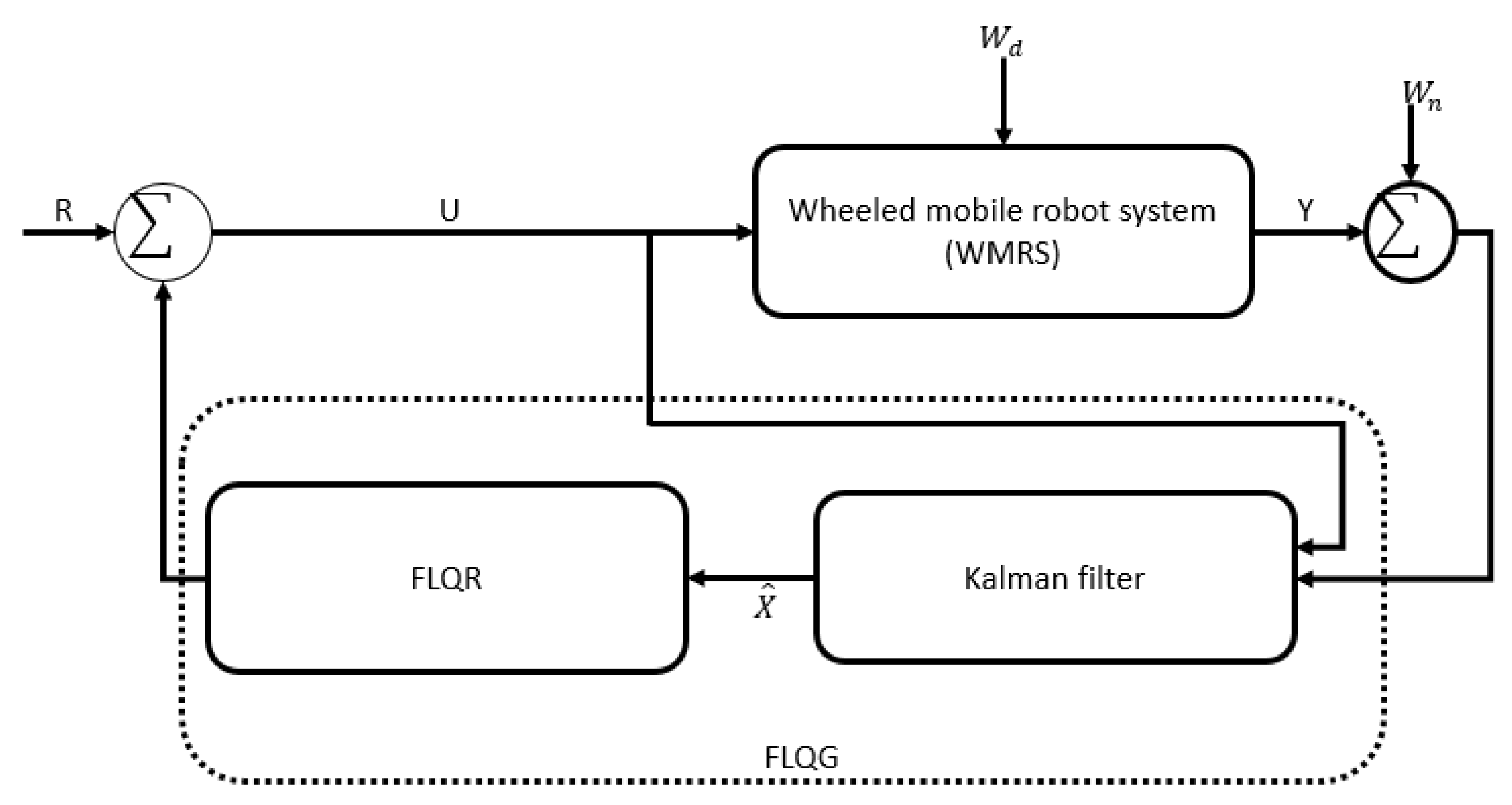
- Linear quadratic Gaussian (LQG)
- C.
- Fuzzy linear quadratic Gaussian controller (FLQG)
3.3. Hybridization Control Gain Design
3.4. Dynamics of WMRS Characters Parameter Analysis
3.5. Lorenz System and Its Analyses for the WMRS Controller Framework
4. Results and Discussion
4.1. Temperature Extremes
4.2. Humidity and Moisture
4.3. Vibration and Shock
4.4. Power Fluctuations
- Designed with components and materials rated for the expected environmental stresses
- Housed in rugged, sealed enclosures to protect internal electronics
- Programmed with failsafe mechanisms and fault-tolerant control algorithms
- Regularly tested and maintained to identify and address any degradation in performance
5. Conclusions
Funding
Authors’ Contributions
Availability of Supporting Data
Acknowledgments
Conflict of interests
References
- S. Amertet, G. Gebresenbet, H. M. Alwan, and K. O. Vladmirovna, “Assessment of Smart Mechatronics Applications in Agriculture: A Review,” Appl. Sci., vol. 13, no. 12, p. 7315, 2023.
- M. Faiz, B. Sumantri, and B. S. B. Dewantara, “Double Loop Controller of Four Mecanum-Wheel Automated Guided Vehicle using SMC-PID,” in 2023 International Electronics Symposium (IES), IEEE, 2023, pp. 305–310. Accessed: Feb. 11, 2024. [Online]. Available: https://ieeexplore.ieee.org/abstract/document/10242526/.
- R. Shamshiri and W. I. Wan Ishak, “Design and simulation of control systems for a field survey mobile robot platform.,” Res. J. Appl. Sci. Eng. Technol., vol. 6, no. 13, pp. 2307–2315, 2013.
- An et al., “EASS: An automatic steering system for agricultural wheeled vehicles using fuzzy control,” Comput. Electron. Agric., vol. 217, p. 108544, 2024.
- C. Luo et al., “Design and Evaluation of Field Segmentation, Path Generation and Sequential Point Tracking Algorithms for Agricultural Mobile Robots,” J. ASABE, p. 0, 2024.
- Yoo, D. Baek, and S. Choi, “Navigation Path Following Platform for a Greenhouse Shuttle Robot Using the State-flow Method,” Math. Probl. Eng., vol. 2024, 2024, Accessed: Feb. 25, 2024. [Online]. Available: https://www.hindawi.com/journals/mpe/2024/8810990/.
- H. Kang, C.-W. Park, and C.-H. Hyun, “Alternative identification of wheeled mobile robots with skidding and slipping,” Int. J. Control Autom. Syst., vol. 14, no. 4, pp. 1055–1062, Aug. 2016. [CrossRef]
- S. Amertet, G. Gebresenbet, and H. M. Alwan, “Optimizing the performance of a wheeled mobile robots for use in agriculture using a linear-quadratic regulator,” Robot. Auton. Syst., p. 104642, 2024.
- Emmi, R. Fernández, and P. Gonzalez-de-Santos, “An Efficient Guiding Manager for Ground Mobile Robots in Agriculture,” Robotics, vol. 13, no. 1, p. 6, 2023.
- R. Shamshiri and W. I. W. Ismail, “Control system design for a field survey agricultural mobile robot,” in International Conference on Agricultural and Food Engineering for Life (Cafei2012), 2012, p. 28. Accessed: Feb. 11, 2024. [Online]. Available: https://www.researchgate.net/profile/Redmond-Shamshiri/publication/280093083_Control_System_Design_for_a_Field-Survey_Agricultural_Mobile_Robot/links/55a8467e08aea994671dd8b5/Control-System-Design-for-a-Field-Survey-Agricultural-Mobile-Robot.pdf.
- R. Cale, “Modeling and Control of a Four-wheel Autonomous Agricultural Robot,” Master’s Thesis, NTNU, 2021. Accessed: Feb. 11, 2024. [Online]. Available: https://ntnuopen.ntnu.no/ntnu-xmlui/bitstream/handle/11250/2787895/no.ntnu:inspera:76427839:20997435.pdf?sequence=1.
- X. Tu, “Robust navigation control and headland turning optimization of agricultural vehicles,” PhD Thesis, Iowa State University, 2013. Accessed: Feb. 25, 2024. [Online]. Available: https://search.proquest.com/openview/2e57452e00a58cd99d9cb79572008df4/1?pq-origsite=gscholar&cbl=18750.
- X. Li and M. Wang, “Consensus control for wheeled mobile robots under input saturation constraint,” IEEE Access, vol. 8, pp. 177125–177130, 2020.
- C. Moon and W. Chung, “Kinodynamic planner dual-tree RRT (DT-RRT) for two-wheeled mobile robots using the rapidly exploring random tree,” IEEE Trans. Ind. Electron., vol. 62, no. 2, pp. 1080–1090, 2014.
- H. Yang, X. Fan, P. Shi, and C. Hua, “Nonlinear control for tracking and obstacle avoidance of a wheeled mobile robot with nonholonomic constraint,” IEEE Trans. Control Syst. Technol., vol. 24, no. 2, pp. 741–746, 2015.
- Ryu, J. Won, H. Chae, H. S. Kim, and T. Seo, “Evaluation Criterion of Wheeled Mobile Robotic Platforms on Grounds: A Survey,” Int. J. Precis. Eng. Manuf., vol. 25, no. 3, pp. 675–686, Mar. 2024. [CrossRef]
- Kamon et al., “Energy Consumption of a Wheel/Track Reconfigurable Mobile Robot on the Farm,” in 2024 IEEE/SICE International Symposium on System Integration (SII), IEEE, 2024, pp. 798–803. Accessed: Feb. 25, 2024. [Online]. Available: https://ieeexplore.ieee.org/abstract/document/10417300/.
- D. A. V. Trinh and N. T. Thinh, “A Study of an Agricultural Indoor Robot for Harvesting Edible Bird Nests in Vietnam,” AgriEngineering, vol. 6, no. 1, pp. 113–134, 2024.
- J. Qu, Z. Zhang, Z. Qin, K. Guo, and D. Li, “Applications of Key Autonomous Navigation Technologies for Unmanned Agricultural Tractors: A Review,” 2024, Accessed: Feb. 25, 2024. [Online]. Available: https://www.preprints.org/manuscript/202402.0401.
- Yuan, Y. Liu, Y.-H. Liu, and C.-Y. Su, “Differential flatness-based adaptive robust tracking control for wheeled mobile robots with slippage disturbances,” ISA Trans., vol. 144, pp. 482–489, 2024.
- K. Wang, Z. Xu, K. Zhang, Y. Huang, and J. Xu, “Lattice piecewise affine approximation of explicit nonlinear model predictive control with application to trajectory tracking of mobile robot,” IET Control Theory Appl., vol. 18, no. 2, pp. 149–159, Jan. 2024. [CrossRef]
- Mehallel, L. Mérida-Calvo, R. Rivas-Perez, and V. Feliu-Batlle, “A New Smith Predictor Motor Control System to Reduce Disturbance Effects Caused by Unknown Terrain Slopes in Mobile Robots,” in Actuators, MDPI, 2024, p. 46. Accessed: Feb. 25, 2024. [Online]. Available: https://www.mdpi.com/2076-0825/13/2/46.
- D. Dirckx, M. Bos, B. Vandewal, L. Vanroye, W. Decré, and J. Swevers, “ASAP-MPC: An Asynchronous Update Scheme for Online Motion Planning with Nonlinear Model Predictive Control.” arXiv, Feb. 09, 2024. Accessed: Feb. 25, 2024. [Online]. Available: http://arxiv.org/abs/2402.06263.
- M. Ahsan and M. M. Salah, “Improved nonlinear model predictive control with inequality constraints using particle filtering for nonlinear and highly coupled dynamical systems,” Nonlinear Eng., vol. 13, no. 1, p. 20220351, Feb. 2024. [CrossRef]
- O. Y. Ismael, M. Almaged, and A. I. Abdulla, “Nonlinear Model Predictive Control-based Collision Avoidance for Mobile Robot,” J. Robot. Control JRC, vol. 5, no. 1, pp. 142–151, 2024.
- Y. Tang, S. Qi, L. Zhu, X. Zhuo, Y. Zhang, and F. Meng, “Obstacle Avoidance Motion in Mobile Robotics,” J. Syst. Simul., vol. 36, no. 1, p. 1, 2024.
- Y. Zheng, J. Zheng, K. Shao, H. Zhao, H. Xie, and H. Wang, “Adaptive trajectory tracking control for nonholonomic wheeled mobile robots: A barrier function sliding mode approach,” IEEECAA J. Autom. Sin., 2024, Accessed: Feb. 25, 2024. [Online]. Available: https://ieeexplore.ieee.org/abstract/document/10379559/.
- Y. Zheng, J. Zheng, K. Shao, H. Zhao, Z. Man, and Z. Sun, “Adaptive fuzzy sliding mode control of uncertain nonholonomic wheeled mobile robot with external disturbance and actuator saturation,” Inf. Sci., p. 120303, 2024.
- T. Zhao, P. Qin, S. Dian, and B. Guo, “Fractional order sliding mode control for an omni-directional mobile robot based on self-organizing interval type-2 fuzzy neural network,” Inf. Sci., vol. 654, p. 119819, 2024.
- M. Y. Silaa, A. Bencherif, and O. Barambones, “Indirect Adaptive Control Using Neural Network and Discrete Extended Kalman Filter for Wheeled Mobile Robot,” in Actuators, MDPI, 2024, p. 51. Accessed: Feb. 25, 2024. [Online]. Available: https://www.mdpi.com/2076-0825/13/2/51.
- M. Rybczak, N. Popowniak, and A. Lazarowska, “A Survey of Machine Learning Approaches for Mobile Robot Control,” Robotics, vol. 13, no. 1, p. 12, 2024.
- R. S. Patil, S. P. Jadhav, and M. D. Patil, “Review of Intelligent and Nature-Inspired Algorithms-Based Methods for Tuning PID Controllers in Industrial Applications,” J. Robot. Control JRC, vol. 5, no. 2, pp. 336–358, 2024.
- A. Nada and M. A. Bayoumi, “Development of embedded fuzzy control using reconfigurable FPGA technology,” Automatika, vol. 65, no. 2, pp. 609–626, Apr. 2024. [CrossRef]
- F. Zafar et al., “Stabilization and tracking control of underactuated ball and beam system using metaheuristic optimization based TID-F and PIDD2–PI control schemes,” Plos One, vol. 19, no. 2, p. e0298624, 2024.
- Li, C. Ma, Y.-H. Chen, and R. Yu, “Stratified Game-Theoretic Optimization of Robust Control Design for Fuzzy Dynamical Systems: A Hybrid Nash–Stackelberg Strategy,” IEEE Trans. Syst. Man Cybern. Syst., 2024, Accessed: Feb. 25, 2024. [Online]. Available: https://ieeexplore.ieee.org/abstract/document/10384797/.
- T. V. A. Nguyen and N. H. Tran, “A TS Fuzzy Approach with Extended LMI Conditions for Inverted Pendulum on a Cart,” Eng. Technol. Appl. Sci. Res., vol. 14, no. 1, pp. 12670–12675, 2024.
- “Development of a Fuzzy-LQR and Fuzzy-LQG stability... - Google Scholar.” Accessed: Feb. 25, 2024. [Online]. Available: https://scholar.google.com/scholar?hl=en&as_sdt=0%2C5&as_ylo=2024&scioq=Optimizing+the+performance+of+a+wheeled+mobile+robots+for+use+in+agriculture+using+a+linear-quadratic+regulator&q=Development+of+a+Fuzzy-LQR+and+Fuzzy-LQG+stability+control+for+a+double+link+rotary+inverted+pendulum&btnG=.

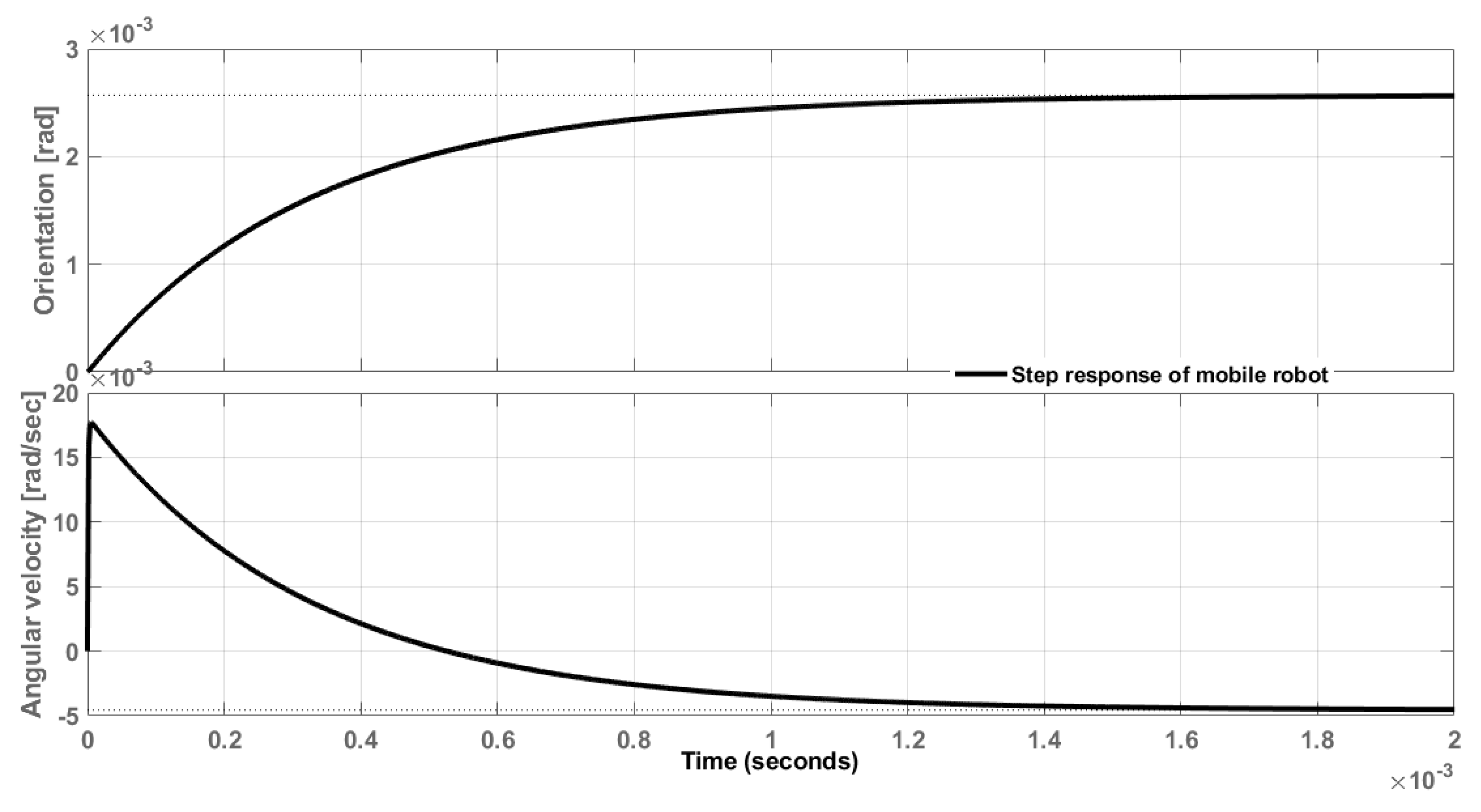
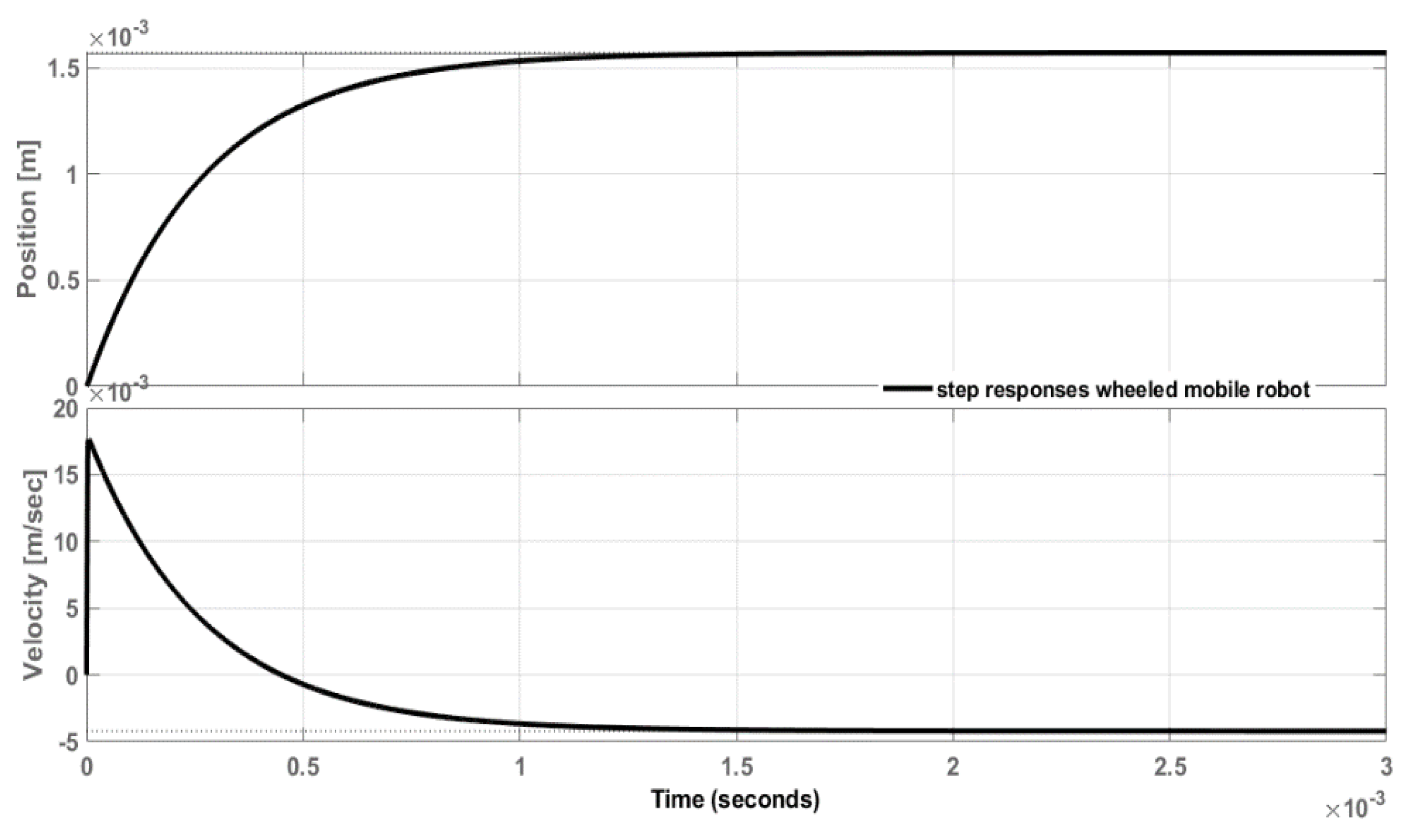
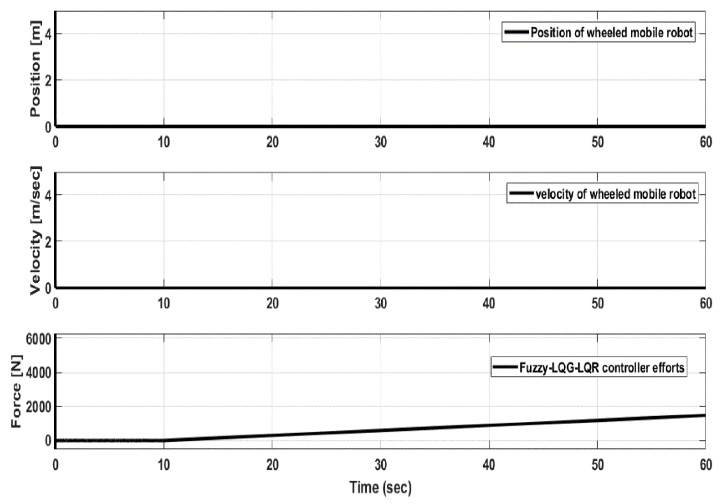
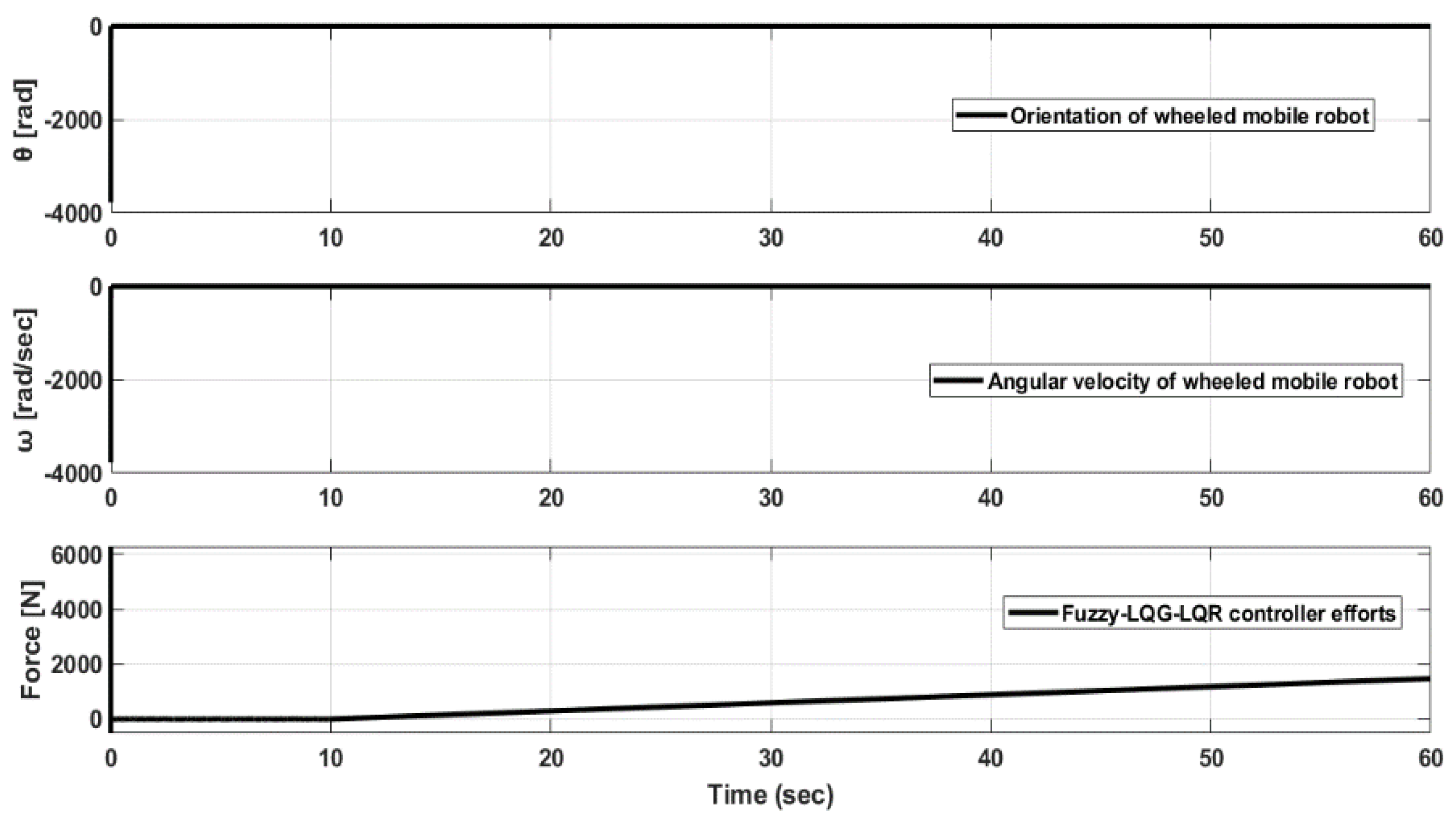
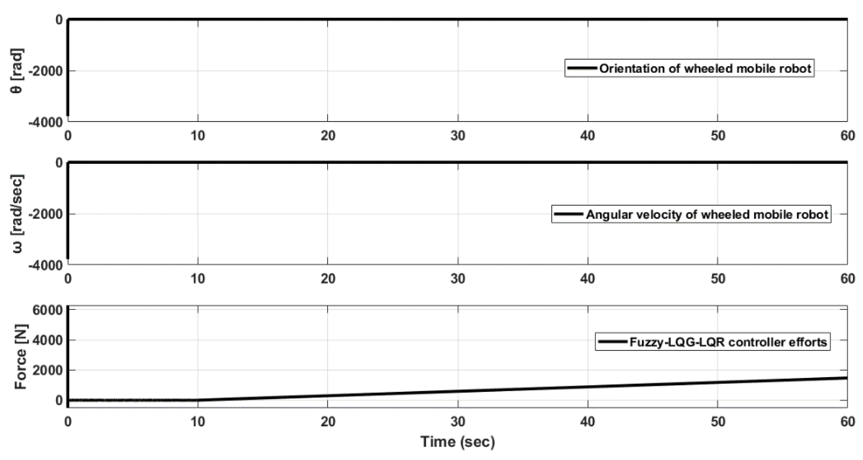
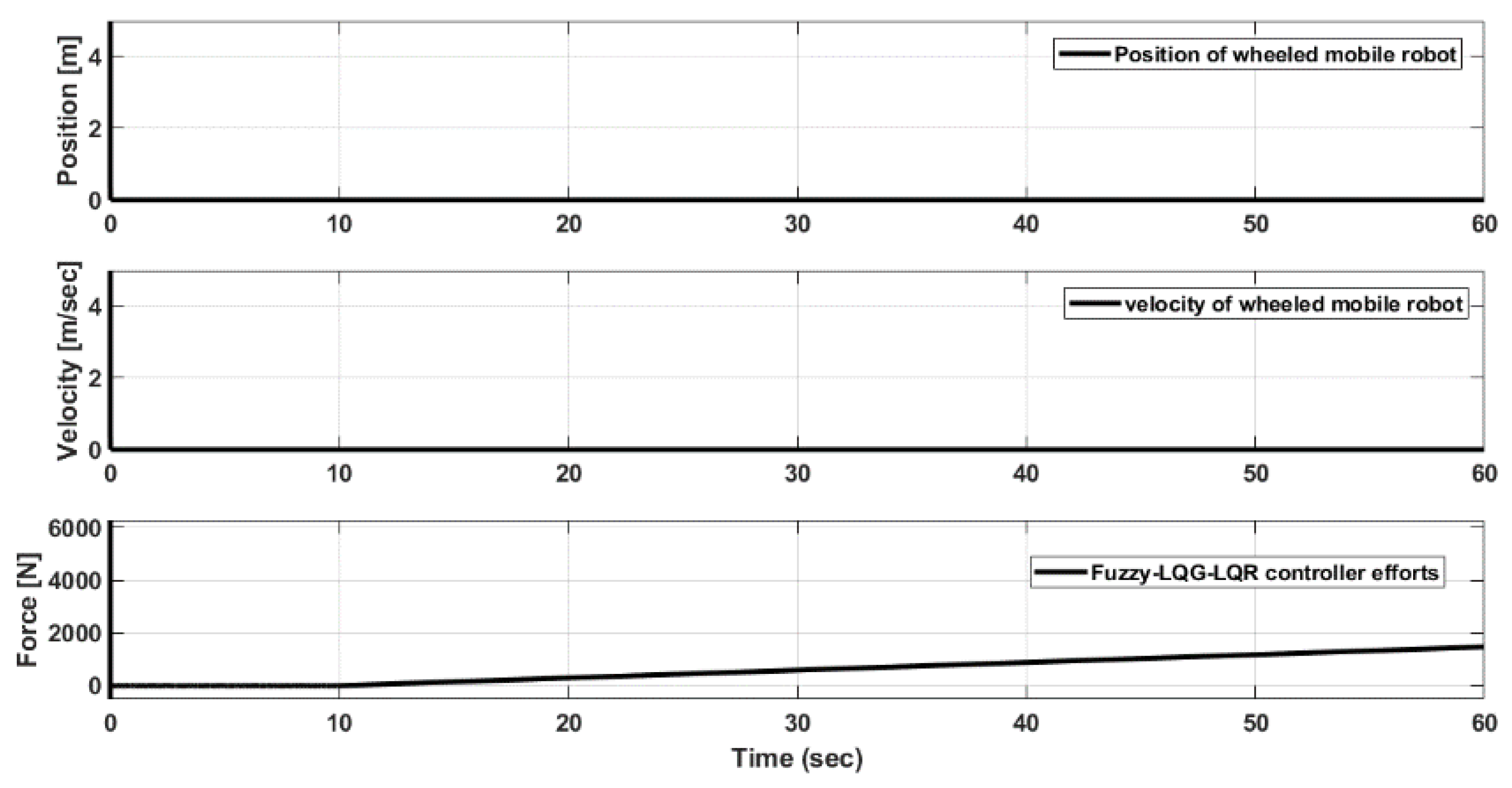
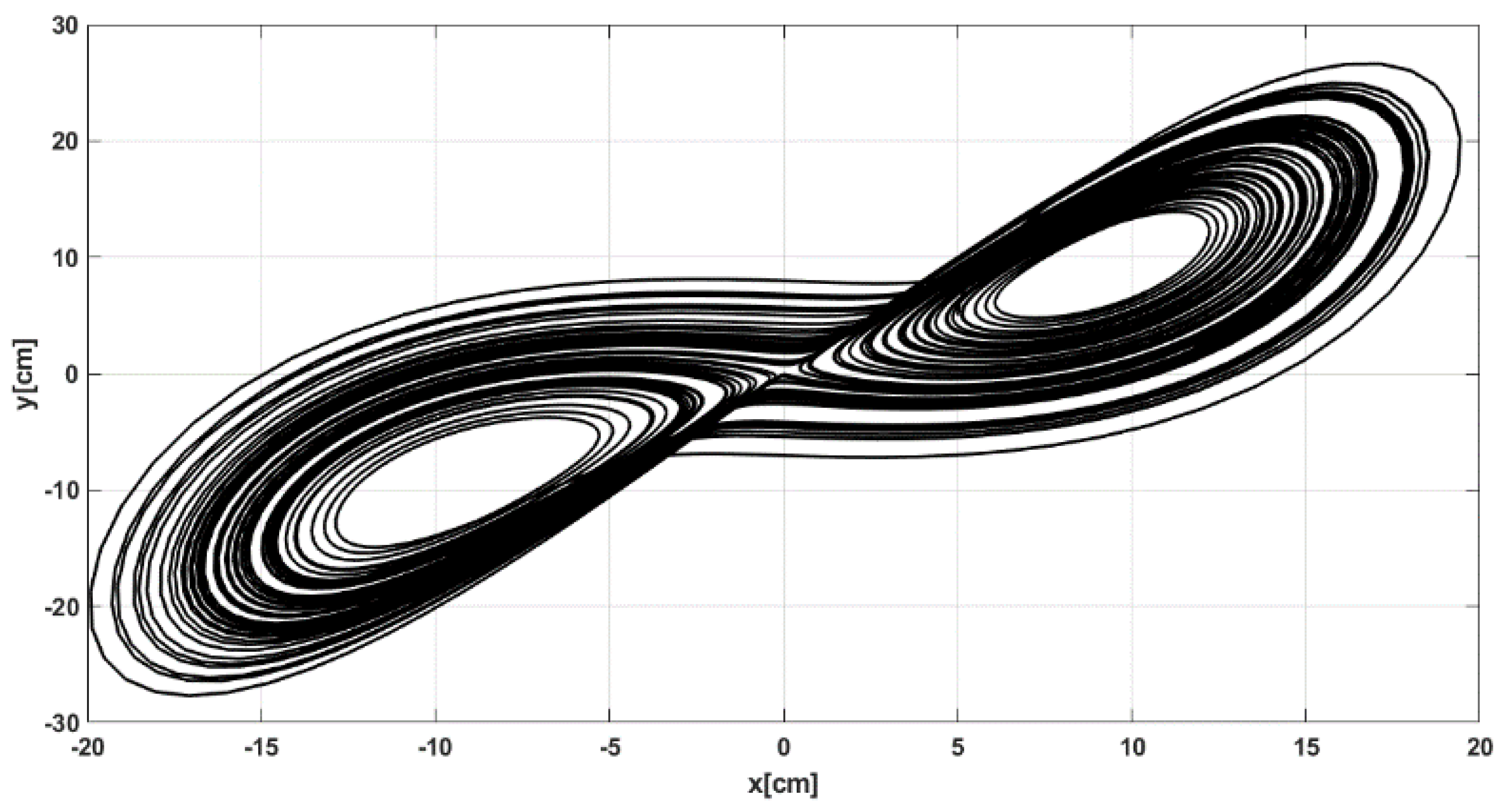
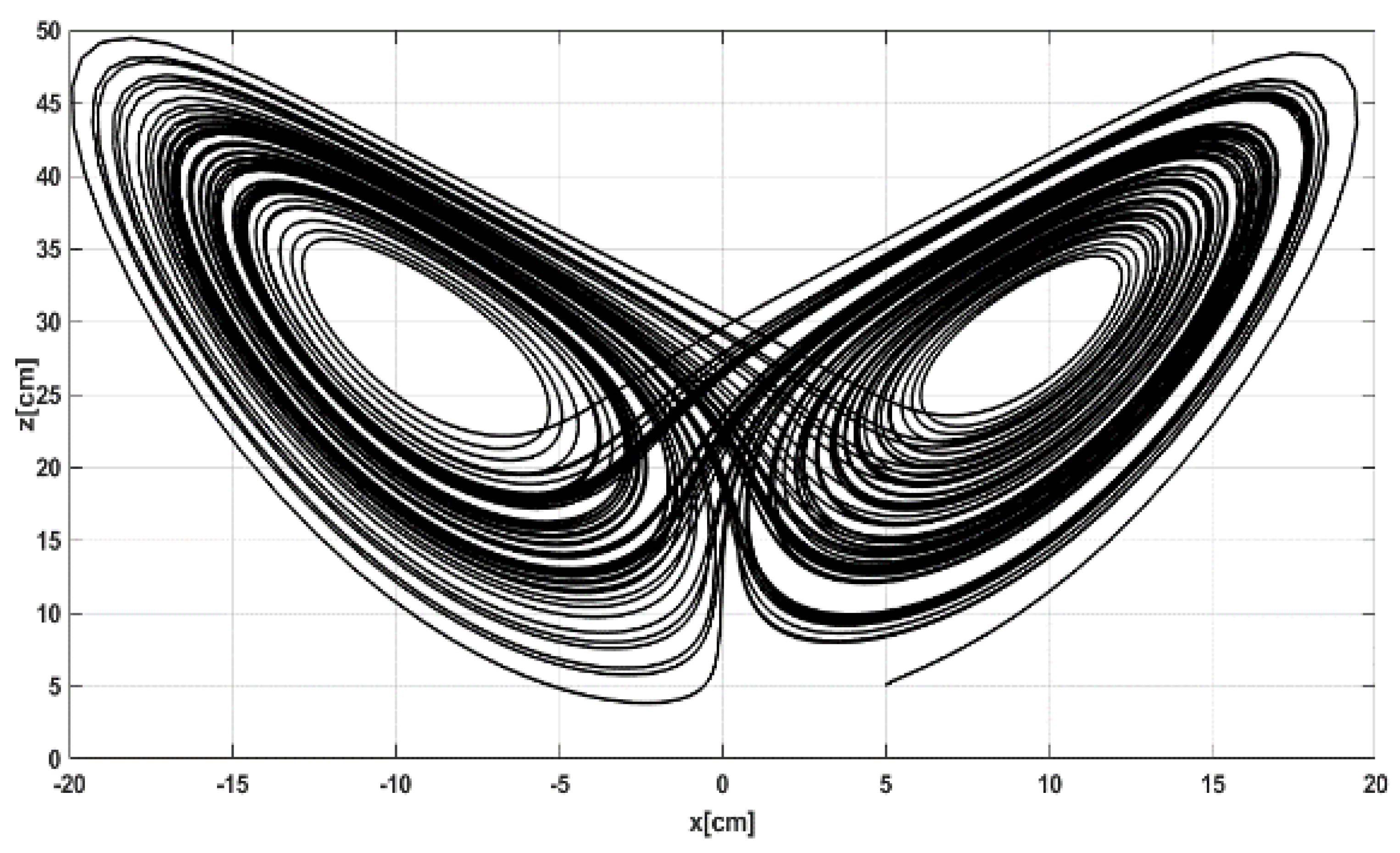
| EC | |||||||
|---|---|---|---|---|---|---|---|
| E | NB | NM | NS | ZE | PS | PM | PB |
| NB | NB | NB | NB | NM | NM | NS | ZE |
| NM | NB | NB | NM | NM | NS | ZE | PS |
| NS | NB | NM | NM | NS | ZE | PS | PM |
| ZE | NM | NM | NS | ZE | PS | PM | PM |
| PS | NM | NS | ZE | PS | PM | PM | PB |
| PM | NS | ZE | PS | PM | PM | PB | PB |
| PB | ZE | PS | PM | PB | PB | PB | PB |
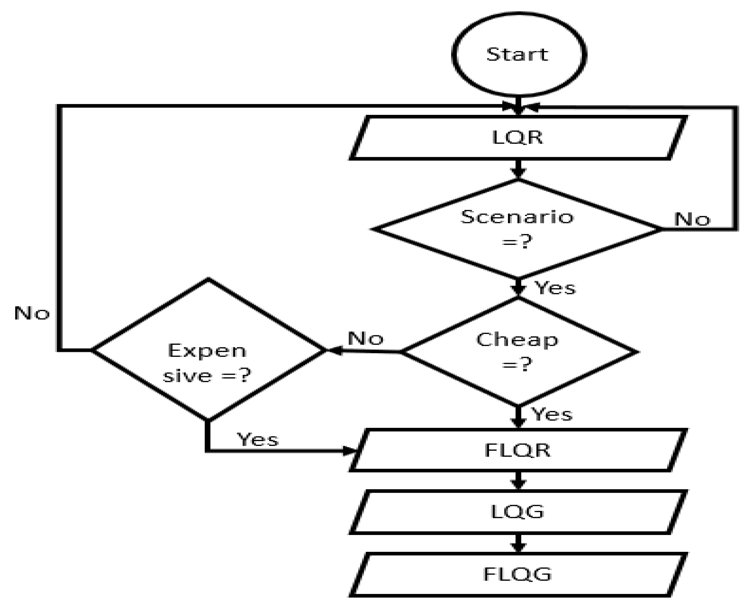
| Scenarios | Penalisation rate (KR) | Penalisation rate (KE) | Eigen values (E) |
| Cheap controller | |||
| Expensive controller | |||
| Ignore anyone state controller |
| Specifications | Error by LQR | Error by LQG | Error by FLQG | %FLQG over LQR | %FLQG over LQG |
|---|---|---|---|---|---|
| Steady state error [%] | 0.001 | 0.000998 | 0.0000023 | 99.77 | 99.76 |
| Peak amplitude [m/sec] | 0.1 | 0.0998 | 0.023 | 77 | 76.9 |
| Settling time [sec] | 0.782 | 0.781 | 0.1 | 87.2 | 87.1 |
| Rise time [sec] | 0.439 | 0.439 | 0.137 | 68.8 | 68.8 |
| Overshoot [%] | 0 | 0 | 0 | 0 | 0 |
| Parameters | Error FLQG cheap control | Error FLQG expensive control | ||||||
|---|---|---|---|---|---|---|---|---|
| Position [cm] |
Orientation [rad] |
Velocity [m/sec] |
Angular velocity [rad/sec] |
Position [cm] |
Orientation [rad] |
Velocity [m/sec] |
Angular velocity [rad/sec] |
|
| Step input | 0.3493 | 0.3498 | 0.02088 | 0.02088 | 0.0006608 | 0.0006642 | 0.0005642 | 0.0005642 |
| Double pulse input | 0.3493 | 0.3498 | 0.02088 | 0.02088 | 0.0006608 | 0.0006642 | 0.0005642 | 0.0005642 |
| Square input | 0.3493 | 0.3498 | 0.02088 | 0.02088 | 0.0006608 | 0.0006642 | 0.0005642 | 0.0005642 |
Disclaimer/Publisher’s Note: The statements, opinions and data contained in all publications are solely those of the individual author(s) and contributor(s) and not of MDPI and/or the editor(s). MDPI and/or the editor(s) disclaim responsibility for any injury to people or property resulting from any ideas, methods, instructions or products referred to in the content. |
© 2024 by the authors. Licensee MDPI, Basel, Switzerland. This article is an open access article distributed under the terms and conditions of the Creative Commons Attribution (CC BY) license (http://creativecommons.org/licenses/by/4.0/).


