
You are currently viewing a beta version of our website. If you spot anything unusual, kindly let us know.
Preprint
Article
The Small and Moderate Earthquake Parameters Training Catalog on the Main Faults in Sichuan, China
Altmetrics
Downloads
96
Views
23
Comments
0

This version is not peer-reviewed
Abstract
Numerous investigations have suggested that seismic source parameters and properties of the surrounding medium harbor valuable information regarding alterations in stress fields and medium properties at the focal depth. Monitoring the spatial and temporal evolution of these parameters can yield insights into variations in stress fields or medium properties within the seismogenic zone, offering a critical avenue to overcome the Earth's inaccessible nature. In recent years, modern seismic parameters such as seismic moment, focal mechanism solution, source stress drop, corner frequency, radiated seismic energy, rupture radius, and apparent stress have been increasingly used to characterize source characteristics. The Sichuan region is situated on the southeastern edge of the Qinghai-Tibet Plateau and is known for its strong eastward extrusion and structural deformation. The main fault zones in the area include the Xianshuihe Fault, Anninghe Zemuhe Fault, and Longmenshan Fault. This paper estimates source parameters of small to medium-sized earthquakes (ML 1.5-5.2) in the main fault zones and adjacent areas in Sichuan. A total of 4,310 earthquake stress drop measurements from 2019 to 2023 were analyzed to create a stress distribution image along the fault. This earthquake parameters training catalog provides insight into how coseismic stresses change and their relationship with other geophysical factors, as well as their spatial and temporal evolution.
Keywords:
Subject: Environmental and Earth Sciences - Geophysics and Geology
1. Introduction
The earthquake process involves two fundamental interrelated links: the tectonic background and the seismogenic environment. The tectonic background refers to the large-scale dynamic energy required for earthquake occurrence, while the seismogenic environment pertains to local conditions under which strong earthquakes occur. It depends on the physical properties of the medium, tectonic activity, and stress state of the location where the earthquake occurs [1,2].
Earthquakes are the result of sudden instability and rupture caused by the continuous accumulation of strain in discontinuous deformation areas, ultimately reaching the limit state under regional tectonic stress provided by the tectonic background [3]. Non-continuous structural areas are often where strain is most easily accumulated and structural deformation is strongest, making them favorable locations for strong earthquake development.
Experiments in Structural Physics [4,5,6,7,8] have indicated that main-aftershock type earthquakes predominantly occur in homogeneous medium environments. In contrast, fore-main-aftershock type earthquakes and swarm type earthquakes tend to occur in complex tectonic environments. Analysis of the modern tectonic stress field and intense seismic activity suggests a significant correlation between stress distribution and the occurrence as well as recurrence of earthquakes.
On the one hand, regions experiencing strong and complex tectonic stress, as well as changes in the direction and type of stress, are more susceptible to powerful earthquakes. It is common for large earthquakes to occur in areas where there is a relatively high accumulation of stress within active fault zones or in sections where fault zones are relatively locked; On the contrary, the local stress variation area in a uniform stress field background is an area where strong seismic activity is relatively concentrated. Under specific conditions, even a small stress variation of 0.1 bar magnitude can significantly impact seismic activity. Research conducted by Xu et al. [9] has indicated that faults capable of generating high magnitude earthquakes often exhibit low b-values and high stress anomaly segments. Additionally, their pre-earthquake locking characteristics are essential prerequisites for stress or strain accumulation and the occurrence of high magnitude earthquakes.\
The type of earthquake sequence is also influenced by the overall level of stress. Isolation-type earthquakes typically occur under conditions of high prestress and/or low rupture strength, while front-main-residual type earthquake sequences tend to occur under conditions of medium prestress and/or medium rupture strength. Additionally, swarm-type earthquake sequences are associated with low prestress and/or high rupture strength conditions [10].
When utilizing seismological methods to assess the risk of significant earthquakes within a research area, the M6.0 earthquake in Parkfield in 2004 serves as a typical illustration. Allmann and Shearer [11] emphasized that enhanced stress is often observed in fault areas prior to a strong earthquake, and there is a substantial decrease in regional stress drop following the event. Hardebeck and Aron [12] proposed that regions with higher strength or subjected to greater external shear stress are more likely to exhibit higher source stress drop, and areas with concentrated distribution of high stress drop may serve as potential nucleation sites for moderate to large magnitude earthquakes.
In addition, stress intensity provides crucial information regarding the potential energy release of earthquakes, while stress characteristics offer insights into the possible types of earthquakes. Tensile stress indicates regions under tension and suggests a potential occurrence of earthquakes on normal faults; compressive stress points to areas under compression, indicating a likelihood of earthquakes on reverse faults; neutral stress implies a strike-slip earthquake. Therefore, conducting quantitative research on the state of stress and its variations in the deep seismogenic layer is an essential method for investigating the issue of predicting strong earthquakes.
Due to challenges such as the difficulty in accessing the Earth’s interior and the infrequency of large earthquakes, direct measurement of stress and intensity in the deep crust remains elusive for humans. Numerous studies have indicated that earthquake source parameters and medium properties contain valuable information about changes in stress fields and medium properties at the focal depth. Monitoring the spatio-temporal evolution of these parameters can provide insights into changes in stress fields or medium properties within the seismogenic zone, offering an important means to overcome the Earth’s inaccessibility.
Scientists use various physical parameters to describe an earthquake, and these parameters that depict the mechanical characteristics of the source are known as the source mechanical parameters, abbreviated as the source parameters. Traditional “earthquake statistics” typically only focus on the “time, space, and intensity” sequence of earthquakes. In recent years, modern seismic parameters such as seismic moment, focal mechanism solution, source stress drop, corner frequency, radiated seismic energy, rupture radius, and apparent stress have been increasingly utilized to characterize source characteristics.
A plethora of earthquake examples indicate that the physical properties of large earthquakes differ from those of small and moderate earthquakes in actual earthquake processes. The source characteristics of the former largely reflect the seismic tectonic background, stress mode of the source, and result in a larger rupture area, while small and moderate earthquakes more so reflect non-uniform changes in stress state within a smaller area. The study of source parameters of small and moderate earthquakes not only serves as the basis for exploring the source process of large earthquakes but also provides new insights for studying regional stress states and evaluating potential earthquake magnitudes.
The Sichuan region (Figure 1) is situated on the southeastern edge of the Qinghai-Tibet Plateau and is known for its strong eastward extrusion and structural deformation. The main fault zones in the area include the Xianshuihe Fault [13], Anninghe Zemuhe Fault, and Longmenshan Fault. Over an extended period of geological evolution, this research region has undergone complex structural deformation, leading to a diverse seismic activity behavior within a dynamic environment.
The gray circle represents the background seismic event, while the orange circle signifies the seismic event that is involved in the calculation of source parameters. Additionally, the blue box indicates the six main tectonic areas in Sichuan.
Sichuan is an important area for strong earthquake monitoring in China, with at least 15 earthquakes of magnitude ≥ 7 occurring in just over 200 years. There are significant differences in the seismic activity characteristics of the regional main and secondary faults. Strong earthquakes of magnitude ≥7 mostly occur on the Xianshuihe fault. No earthquakes of magnitude ≥ 7 have occurred on the Anninghe fault since 1536, the Zemuhe fault since 1850, the Jinshajiang fault since 1870, or the Litang fault since 1948. Therefore, understanding the changes in stress state among different faults within this research area has become a focus of attention.
To understand the current stress distribution characteristics of the primary active faults in the region and identify sections where relatively high stress accumulation is occurring, this paper estimates the source parameters of small and medium-sized earthquakes (ML 1.5-5.2) in the main fault zones and adjacent areas in Sichuan. A total of 4,310 measurements of earthquake stress drops during the 5-year period from 2019 through 2023 are analyzed to draw a stress distribution image along the fault. The study discusses the stress distribution characteristics on major faults, variations of seismic stress drop with location, and correlations between stress-strain loading and regional deformation dynamic processes based on geometric structure, activity habits, and temporal spatial distribution of modern seismic activity in different sections of the region. This earthquake parameters training catalog provides an opportunity to understand how coseismic stresses change and how other geophysical factors relate to the distribution of stress drop as well as its evolution in space and time.
2. Main Fault Zones and Their Activity
2.1. Longmenshan Fault Zone (LMS)
The Longmenshan fault zone is located on the eastern edge of the Qinghai Tibet Plateau, at the junction of the Bayankala block and the Yangtze block. The Longmenshan fault zone has four main faults developing from northwest to southeast: the Maoxian Wenchuan Fault (Houshan Fault), the Beichuan Yingxiu Fault (Central Fault), the Jiangyou Guanxian Fault (Qianshan Fault), and the Guangyuan Dayi Fault (Hidden Fault in front of the Mountain). The dextral strike slip rate (<1mm/a) and vertical slip rate (<1mm/a) of the Longmenshan fault zone are both very small [14,15], and multiple periods of sliding have occurred. The secondary fault exhibits long-term creep deformation characteristics [16,17].
The 2008 Wenchuan 8.0 earthquake occurred on the Longmenshan Fault zone, causing both the Beichuan Yingxiu Fault (Central Fault) and the Jiangyou Guanxian Fault (Qianshan Fault) to rupture simultaneously. The surface rupture zone of the central fault is about 240km long, mainly characterized by reverse fault displacement, and also has a right lateral strike slip component. The surface rupture of the Qianshan Fault is about 72km long, which is a typical reverse fault displacement property. The 2013 Lushan 7.0 earthquake occurred in the southern section of the Longmenshan Fault zone, which was a blind reverse fault type earthquake. No structurally significant fractures were found on the surface.
2.2. Xianshuihe Fault (XSH)
The Xianshuihe fault of western Sichuan Province, China, is one of the world’s most active faults, can be divided into two segments of different structural styles, jointing at the pull-apart area of Huiyuan Monastery. The northwestern segment has a relatively simple geometric structure. While the southeastern segment exhibits a complex structure composed of several branches. In the southern part of Huiyuansi, the fault is divided into three secondary parts as Yalahe fault, Selaha fault, and Zheduotang fault. To the south of Kangding, it is manifested as a main fault with only local branching phenomenon, known as the Moxi fault.
The Xianshuihe fault is a highly active strike-slip fault system. Since earthquake records began in 1700, the Xianshuihe fault has experienced eight M>7.0 earthquakes, accounting for about half of the total earthquakes of the same magnitude in the entire western Sichuan region. The surface rupture zone of the earthquake almost covers various sections of the entire fault.
2.3. Jinshajinag Fault (JSJ)
The Jinshajiang fault is composed of multiple SN direction arc-shaped secondary reverse faults and the NNE trending Batang fault. There is almost no seismic activity on the arc-shaped secondary fault. Moderate historical earthquakes have occurred on the west segment of the Batang Fault, such as the earthquakes of 1989 M6.7, 2006 M 5.0, M 5.4 and M 5.6 in Balongda. From the perspective of active structure, the arc-shaped secondary reverse fault is a complex fracture zone composed of numerous small faults and fault combinations, which is not easy to concentrate stress. Seen from Google earth images, the Batang fault has a clear geomorphic expression, however, geometry and late Quaternary slip-rate are still unknown.
2.4. Muli-Yanyuan Fault (MLI)
The active fault system of this unit is mainly composed of the NE oriented Lijiang Xiaojinhe fault zone and secondary faults parallel to it, in addition to the Muli Arc Fault, Zhongdian-Daju Fault, and Ninglang Fault. These main and secondary active faults intersect and intersect locally, resulting in frequent seismic activity in this unit both historically and today. Among them, the Lijiang-Xiaojinhe Fault cuts through the Research diamond block and divides it into two parts: the northwest Sichuan secondary block and the central Yunnan secondary block. The Ninglang-Yanyuan and Muli areas are located at the junction of the south and north secondary blocks.
2.5. Anninghe-Zemuhe Fault Zone (ANH)
The Anninghe Fault zone is located on the axis of the Kangdian earth axis, starting from Shimian in the north and extending through Xichang to the Huili area. It generally runs in an NS direction and is mainly characterized by sinistral strike slip movement. In history, this area may have occurred 1470 AD earthquake.The Mianning-Xichang area in the southern section of the Anninghe fault was the main rupture part of the M 7½ in 1536.But since the M 63/4 earthquake in south of Mianning in 1952, there have been no larger earthquakes on the Anninghe Fault. A modern seismic gap gradually formed with the Liziping-Xichang section as the core, with the background of the first kind seismic gap.
The northern end of the Zemuhe fault is connected to the Anninghe fault, and the southern end is connected to the Xiaojiang fault. It extends from Xichang through Puge and Ningnan to Qiaojia, with an overall trend of 330°. There have been M 7 earthquakes in 814 AD and M 7½ earthquakes in 1850. The most recent moderate earthquake was the Xichang M5.1 earthquake on October 31, 2018. The Zemuhe fault is mainly characterized by sinistral strike slip movement, with a sinistral strike slip rate of about 6.4 ± 0.6 mm/a in the Holocene [13], accompanied by a normal fault dip slip component between Xichang and Puge [18]. In the southwest of Qiaojia, the southernmost fault of the Zemuhe fault zone deviates towards the south southwest direction.
2.6. Daliangshan Fault (DLS)
The Daliangshan fault is left-lateral strike-slip fault approximately 250 km long. The Daliangshan fault has a complex fault geometry characterized, and mainly composed of four secondary faults, including the Yuexi Fault, Puxiong Fault, Butuo Fault, and Jiaotong River Fault. The historic earthquake record is no M≥6.0 strong earthquakes on the Daliangshan fault. But seismic and geological studies have confirmed that the fault has experienced prehistoric strong earthquakes and has the structural conditions for the breeding and occurrence of strong earthquakes [19,20,21].
3. Database
The estimation of source parameters is of great significance to reveal whether the rupture mechanism of large and small earthquakes has the same physical process, and to apply source parameters to the study of earthquake prediction and to understand the physical properties of earthquakes. The effective stress, stress drop, and source size can be estimated by comparing the measured seismic spectrum with the theoretical spectrum [22]. Static stress drop is the simplest method to measure the overall reduction in shear stress caused by sliding of fracture zones [23]. It is the difference between the average shear stress on the fault zone before and after the earthquake, and represents the stress released on the fault plane during the earthquake. Assuming that the static initial shear stress on the fault plane before the earthquake is and the final shear stress on the fault plane after the earthquake is , the static stress is reduced by
The average stress is
Since the stress drop of a real earthquake varies throughout the fault zone, the overall static stress drop is the sliding weighted average of the spatially variable stress drop [23].
The corresponding dynamic stress drop is more complex because the space-time history of stress drop can be quite variable. Any individual part of the fault plane may have a variable stress drop during sliding. Due to the impossibility of reliably inverting seismic waves to determine the complete spatiotemporal process of dynamic stress drop, the simplest viewpoint is that the dynamic stress drop is constant on the spatiotemporal window of fault sliding.
When the earthquake rupture begins to expand, the stress at this point gradually increases to the horizontal stress that the rock can withstand, the rupture occurs at this point. For the region without rupture, is the shear fracture strength of the material or rock. To have broken down, for the two discs of the fault and squeezed together by static friction stress, is the maximum static friction stress. When sliding occurs, the stress decreases from to the dynamic friction stress , and the dynamic friction stress remains unchanged during sliding. As the rupture process on the whole fault surface stops, the stress transitions from the dynamic friction stress to the final stress .
The shear rupture strength, or the difference between the maximum static friction stress and the dynamic friction stress , is called the effective stress
In the Brune [22] disk model, assuming that shear failure occurs simultaneously and , the effective stress is the dynamic stress drop
Seismologists generally use simple constant stress drop model to estimate the seismic stress drop. In the method of estimating stress drop using the scaling relation [24,25], regardless of the details of fault geometry and slip distribution, assuming that the earthquake rupture process is a linear elastic process in semi-infinite space. The basic formula for stress drop is as follows
where is the average displacement that occurs on a fault of length L at the time of the earthquake, is the elastic shear modulus. Since seismic moment (M0) for most large earthquakes can be reliably determined from seismic waves, rewrite the above equation as:
where is the fault shape parameter,, refers to the length of the fault, and refers to the width of the fault. Then
or
is the fault area.From formula (7) and (8), we need three quantities to calculate stress drop: a measurement of the seismic moment (), some estimate of the fault area (A), and then some appropriate choice for the characteristic fault dimension ().
In practice, it is very difficult to determine the characteristics of seismic source rupture. It is common to assume a theoretical rupture model to calculate the stress drop, then different geometric coefficients and fault feature length are taken according to the calculation model [25]. For large earthquakes, the rupture scale in the direction of the fault can be tens to hundreds of kilometers, the depth direction is limited by the focal depth, and generally adopt × rectangular model, taking , then the stress drop is expressed as
For the infinite dip-slip fault model,
is the Lame coefficient.
For small magnitude earthquakes, Brune’s [22] disk rupture model is often used, which assumes that earthquake rupture occurs on a circular fault plane with uniform stress drop and constant rupture velocity. Usually c=7π/16, take the disc radius , stress drop is expressed as
For the acquisition of the rupture radius , the source rupture process can be retrieved from the far-field seismic records in seismology, by the frequency domain of corner frequency indirect access to the source physical dimension information [26,27], expressed as
is the shear velocity near the source.
Then formula (11) is rewritten as
is a constant, depending on the type of model used to correlate the relationship between the corner frequency and the focal rupture radius . In Brune [22] model, ; In the Madariaga [28] model, [29,30]; In Sato and Hirasawa [31], depends on the source rupture velocity [32].
The obtained by equation (13) is proportional to the cube of , so the stress drop is very sensitive to the error of . Even if the fault model is close to the actual fault, the small observation error of will reduce the reliability of , which is also the limitation of the traditional seismological method to give the seismic stress value.
4. Results
4.1. Scaling Relationships of Earthquake Source Parameters
The relationships between earthquake source parameters like seismic moment ,or magnitude , moment magnitude ,stress drop , corner frequency , and source scale r ,are termed as scaling relations [33,34]. The self-similar of earthquakes is manifested on many scales, which means that stress drops remain constant over a large range of earthquake magnitudes, and fault sliding systematically increases with the fracture area. However, other studies have emphasized the possible self-similarity bias at regional and global scales, indicating that stress reduction may vary with earthquake magnitude and different regions [35,36].
Here, we try to unravel measurement uncertainty and potential physical differences in earthquake source processes by analyzing source spectra of more than 4,310 micro-earthquakes ranging from ML 1.5 to ML 5.2 in the 5-yr time period from 2019 through 2023. Analyzing a large number of small-magnitude earthquakes enables us to better resolve statistically significant variations in source parameters, such as stress drops, even if scatter is high. We analyze seismograms, including those of numerous small earthquakes, to calculate the scaling relations of seismic source parameters in six tectonic zones (Table 1).
The moment magnitude reflects the magnitude of deformation and is an absolute mechanical scale for describing earthquake size which does not cause saturation problems. So, it is the best physical quantity for measuring earthquake size currently. By assuming specific models of fault geometry and fracture dynamics, the seismic moment of the source spectrum can be used to determine the size of the fracture. Here in six tectonic zones, as the moment magnitude increases, the source scale increases linearly (Figure 2).
Both local magnitude and seismic moment or equivalently moment magnitude are measures of basic properties of the earthquake source: is proportional to the maximum of the moment-rate function, whereas is proportional to its integral. Thus, theoretical considerations and empirical regressions show that, the values of and should be the same for special earthquakes caused by similar source processes. However, the observed data do not match the ideal situation.
The observation that the theoretical 1:1 relationship breaks down in empirical relationships was explored by Hanks and Boore [37]. Ben-Zion and Zhu [38] proposed that an alternative cause of the deviation from 1:1 scaling could result from non-self-similarity of earthquake sources. For small events the heterogeneity of a tectonic stress field may lead to slip that does not grow substantially with rupture dimension, whereas for larger events the effect of small-scale stress heterogeneities is smoothed out. That means the evolution between the two extremes of small and large events could lead to the observed polynomial form of - scaling.
In our research,a difference was also observed between and . We performed linear regressions for versus in different areas (Figure 3), and found that for small magnitude events, this 1:1 relationship is ineffective. However,from these data we observed systematic deviations of relative to , simultaneously fitting the linear scaling relationship between and . The determination of for small events is desirable to obtain robust a and b values in a recurrence relationship and the magnitude of completeness of the earthquake catalogue.
To improve our understanding of these differences between and , some studies suggest that it can be attributed to the variation in the physical properties, as attenuation and scattering along the path, pore fluid pressure, temperature, and related changes in normal stress, interface morphology, and material properties [39,40].
4.2. Stress Drops Training Catalog
Stress drop is a basic parameter that describes the characteristics of the source scale. Earthquake stress drop is defined as the difference in average shear stress on the fault plane before and after an earthquake, representing the stress released on the fault plane during the earthquake. This study aims to investigate the spatio-temporal distribution of static stress drop values of the six faults rupture seismic sequence in Sichuan. We observe that the vast majority of earthquakes have stress drop between 0.1 and 1 MPa, some earthquakes are between 1 MPa and 10MPa, a few earthquakes have stress drop less than 0.1MPa, only few events are greater than 10MPa (Figure 5). We find several anomalous events with unusually high or low stress drops in the small earthquake parameters training catalog. Individual event stress drops show some scatter. Previous studies [11] have suggested that this divergence presumably caused by inherent uncertainty in the computation method and a combination of other effects, including uncertainty in corner frequency estimation, incomplete averaging of radiation pattern effects,heterogeneities in the physical properties of faults and simplified assumptions about the source model.
Given these sources of uncertainty, it should not be assumed that a single stress drop estimate for a particular event can be generalized to an entire region. Analyzing a large number of small-magnitude earthquakes enables us to better resolve statistically significant variations in stress drops even if scatter is high. In our study, the stress drop was calculated using the same analytical methods and the same source model assumptions for each earthquake in separate tectonic area, so their relative values should be meaningful. We therefore focus on the properties of the data set to obtain statistically significant differences in stress drop to study the relative stress drop between events generated under different tectonic conditions in Sichuan, although the absolute value of the stress drop remains somewhat model dependent. To detect a possible dependence in the highly scattered values, we classify seismic events in different tectonic zones. This classification of events allows us to calculate and investigate median stress drops for each tectonic region. We apply a bootstrap method over 100 resamples for each tectonic region and estimate the median stress drops which represent averages of individual stress drops which are highly scattered. These are listed in Table 2 for each tectonic regime. It is interesting to note that the median stress drop varies with magnitude in different tectonic zones. For most regions, the distribution of stress drops shows a clear peak that allows us to derive meaningful statistics.
Recent observations have suggested that as earthquakes increase in magnitude, they radiate an increasingly large amount of energy [25,43], which implies that stress drop varies with magnitude. We also observed this phenomenon in this study. Although there are actual differences in the spatial patterns of stress drop with seismic moment in different faults (Figure 6), the overall stress drop value for small and medium earthquakes increases with the magnitude increase.
4.3. Spatial Variation of Stress Drops
The spatial distribution of stress drop values in a complex seismic sequence could support a more complete understanding of the earthquake rupture process and the evolution of seismic sequences. It could also highlight areas where stress loading is focused, which would have implications for short and intermediate term seismic hazard estimates [11,29].
Figure 7 shows the individual stress drop estimates at the event locations. At first sight, we observe no obvious correlation with tectonic regime. However, we do observe areas with overall higher or lower average stress drop than their surrounding regions. A particularly striking feature is the region of low stress drop estimates along the XSH fault zone with average values below 2.78 MPa. Examples with higher-than-average stress drops are the ANH fault zone with values around 5.11 MPa and the region near Qiaojia in Yunnan province.
The LMS fault zone shows a very heterogeneous stress drop pattern. We observe an apparent variation along strike with lower stress drop values near the hypocenter of the great Wenchuan earthquake of 2008, and higher stress drops both to the northeast and to the southwest. However, because of the dense clustering of events in this region and a variation of tectonic regimes over short distances, we need to look at a finer regional scale in order to clearly see differences and possible correlations in LMS fault zone.
The stress drop also generally increases with depth [44]. Normal stress on faults increases with depth in the earth and has long been thought to be a potential factor influencing earthquake stress drops [45]. However, some studies have also interpreted the dependence of stress drop on focal depth as an observation illusion [46],which vary significantly along strike [47,48], and to depend on fault rheological and geometrical complexities [49].
We plot the stress drop distribution at a depth of 0-36km in six tectonic zones, and take the depth distribution of the stress drop on the LMS as an example to demonstrate. In order to effectively solve the color matching problem caused by the excessive range of data values, the stress drop data are drawn in Figure 8 after logarithmic selection. In LMS, the high stress drop values are distributed along the fracture trend and mainly occurred from 2019 to 2022. After interpolation along the central fault strike of Longmenshan fault and using the nearest neighbor algorithm to calculate the weighted average of grid points, it is found that stress drop estimates largely constant within the upper 9 km and show a sharp increase at 10km from 3 MPa to 10 MPa. After Delaunay triangulations interpolation [50,51,52,53] of the whole area, the data results show that the high stress drop events are concentrated in the depth range of 20-24km. Even though our study regions in LMS host some of the deepest seismicity in Sichuan, observations of stress drop as a function of depth show considerable variability and the systematic variation of stress drop with depth is not particularly obvious.
5. Discussion
Much research in recent years shows that the average difference in shear stress (static stress drop) on faults caused by earthquakes is usually between 0.1 MPa and 100 MPa [11,29,54,55,56]. In this paper we explore the small earthquake stress drop training catalog on the main faults in Sichuan, the stress drops are usually between 0.1 MPa and 10 MPa. It should be noted that there is considerable scatter in the stress drop estimates above about 30 MPa, which reflects large uncertainties in measuring corner frequencies that are near the 25-Hz upper-frequency limit of our analysis. Thus, these very high values should not be considered reliably resolved although they should be retained in computing median stress drops as they are almost certainly on the high side of the stress drop distribution [55,57,58].
5.1. Self-similar Earthquake Scaling
The source-scaling relationships, including whether stress drop is self-similar and magnitude-invariant [34] or obeys a more nuanced scaling relation. Self-similar earthquake scaling has been observed at many scales, which means that stress drops remain constant across a wide range of magnitudes and that fault slip increases systematically with rupture area [34,59,60]. However, an increase in stress drops with seismic moment would imply non-self-similar earthquake scaling and whether this occurs has been the subject of considerable debate [41,57]. Other studies have emphasized on regional and global scale possible deviation of self-similarity, suggests that stress drops may change with earthquake magnitude in different areas [36]. But source parameter estimates often exhibit a puzzling degree of scatter [57], and results from different methods are often inconsistent, even when using the same underlying data set.
In our study, we have observed a consistent trend of increasing stress drop with magnitude, indicating the presence of self-similarity rule. The same equivalent stress drop line (Figure 5) can traverse at different seismic scales (ordinate), while the fracture scale (abscissa) and seismic moment (ordinate) have the same slope as the stress drop line, which indicates that there is a self-similarity between the fracture scale and seismic moment, and the stress drop can be a constant at different magnitude scales.
It is important to note that the modeling assumptions can significantly impact the absolute values of stress drops, which may not accurately represent the true static stress drop of the earthquake rupture. Our focus in this study is on relative variations in stress drops, which were estimated consistently and can be interpreted as reflecting variations in high-frequency energy release. Higher and lower stress drops correspond to energetic and enervated events, respectively.
5.2. Spatio-Temporal Stress Drop Evolution
In addition to studies exploring systematic variations in stress drop with size, there have been continuous efforts to determine whether stress drop varies based on tectonic environment, faulting mechanism, or focal depth. Recent studies have identified spatial and temporal variations in stress drop in California [11,30,61], Japan [56,62,63], and New Zealand [64]. These papers suggest that spatial and temporal variations of stress drop have the potential to reveal heterogeneities and demonstrate more nuanced changes in the character of a stress field on a fault [12,65]. In this paper, the earthquake sequences are used for detailed studies of spatio-temporal variations in the stress state of the six main tectonic areas with different structural inheritance in Sichuan, to outline regions of alternating high and low stress drop. The relationship between stress drop and faulting regime could help to identify fault segments with relatively high stress accumulations, which generally indicate greater applied shear stresses or the presence of higher-strength materials [12].
From the spatial distribution (Figure 7), we observe that regions of high and low stress drop alternate on either side of the six main tectonic areas. The events with highest stress drop are mostly in the ANH fault zone and the region near Qiaojia in Yunnan province. Our results suggest that the general degree of stress field heterogeneity and strain localization may influence stress drops more strongly,relatively high stress drop estimates correlate with relatively high fault strengths due to inferred low seismic coupling [47] or high fault heterogeneity [44].
Previous studies [66] show that changes in the patterns of high and low stress drop values are in line with the process of stress accumulation or transfer from the pre-mainshock to post-mainshock periods. Taking the LMS fault zone as a case study, we have re-evaluated the stress drop values of small and medium earthquakes occurring from 2013 to 2018 (Figure 9) and from 2019 to 2023 (Figure 10). We have then compared the variations in these values between the two time periods.
In Figure 9, two months after the Ms 7.0 event, the stress drops suddenly attenuate, with significantly less seismic energy release per event. A few high stress drop events occurred in the middle and northern section of LMS fault zone from 2013 to 2015. There are very few high stress drop events between 2019 and 2023. This means that even we observe considerable small-scale heterogeneity, it is still general stability and consistency over the entire time period in LMS fault zone. During the study period, the Lushan 6.0 earthquake also occurred in this area in 2020. We also observed no signicant change in the spatial distribution before and after the 2020 M6.0 earthquake. We deduce from this that the spatial variability in fault conditions is significantly greater than any temporal effects resulting from the coseismic or postseismic slip.
6. Conclusion
The spectral analysis of body waves from 100 Broadband Seismograph (BBS) stations within the Sichuan Seismic Network has been conducted to investigate the scaling relation and self-similarity of small to moderate size earthquakes in Sichuan. These scale relations encapsulate the unique characteristics of the study area and lay a foundation for future predictions of local seismic calibration coefficients in Sichuan. The primary objective behind establishing these scaling relationships is essentially to provide a benchmark against which data can be juxtaposed, thereby serving as a valuable reference point for analysis.
The presence of stress drop scaling and coherent regional variations in source spectral parameters holds profound implications for earthquake physics and seismic hazard assessment. High frequency peak ground motions are, to some extent, contingent upon stress drop, thereby prompting the development of non-ergodic, region-specific ground motion prediction equations to accommodate systematic fluctuations in source parameters. Departures from self-similarity may carry significant ramifications for extrapolating observations of minor earthquakes to constrain the hazards posed by larger ones.
The use of spatial and temporal variation in stress drops as a proxy for the seismic response of fault systems provides an optimal data setting to explore the relationship between fault mechanics, geological setting, and stress drop variation. The spatio-temporal distribution of stress drop values within a complex seismic sequence could potentially provide valuable support for a more comprehensive comprehension of the earthquake rupture process and the development of seismic sequences. Furthermore, it has the potential to identify specific regions where stress loading is concentrated, thus carrying significant implications for short and intermediate-term estimations of seismic hazard.
Author Contributions
Conceptualization, Weiwei Wu and Jun Li; methodology, Feng Long; software, Tian Li and Xianliang Yao; validation, Hong Zuo, Xuefen Chen and Ningbo Jiang; investigation, Mingjian Liang; writing—review and editing, Weiwei Wu and Jun Li; visualization, Jun Li. All authors have read and agreed to the published version of the manuscript.
Funding
This research was funded by NATIONAL KEY RESEARCH AND DEVELOPMENT PROGRAM, grant numbers 2021YFC3000703 and 2021YFC3000602.
Institutional Review Board Statement
Not applicable.
Informed Consent Statement
Not applicable.
Data Availability Statement
The original contributions presented in the study are included in the article, further inquiries can be directed to the corresponding author.
Acknowledgments
We thank reviewers and the editor for their constructive and timely review comments. The figures in this study were generated using the public Generic Mapping Tools (GMT).
Conflicts of Interest
The authors declare no conflicts of interest.
References
- Wang, S. Deformation property recognition of the crust and upper mantle. Seismol. Geol. 1996, 18, 215–224. [Google Scholar]
- Zhang, P. Late Quaternary tectonic deformation and earthquake hazard in continental China. Quat. Sci. 1999, 19, 404–413. [Google Scholar] [CrossRef]
- Ma, J.; Ma, S.L.; Liu, L.Q.; Deng, Z.H.; Ma, W.T.; Liu, T.C. Geometrical textures of faults, evolution of physical field and instability characteristics. Acta Seismol. Sin. 1996, 9, 261–269. [Google Scholar] [CrossRef]
- Kiyoo, M. On the time distribution of aftershocks accompanying the recent major earthquakes in and near Japan. Bull. Earthq. Res. Inst., Univ. Tokyo 1962, 40, 107–124. [Google Scholar]
- Kiyoo, M. Study of elastic shocks caused by the fracture of heterogeneous materials and its relations to earthquake phenomena. Bull. Earthq. Res. Instit. Univ. Tokyo 1962, 40, 125–173. [Google Scholar]
- Scholz, C. Microfractures, aftershocks, and seismicity. Bull. Seismol. Soc. Am. 1968, 58, 1117–1130. [Google Scholar] [CrossRef]
- Scholz, C. Experimental study of the fracturing process in brittle rock. J. Geophys. Res. 1968, 73, 1447–1454. [Google Scholar] [CrossRef]
- Scholz, C. Microfracturing and the inelastic deformation of rock in compression. J. Geophys. Res. 1968, 73, 1417–1432. [Google Scholar] [CrossRef]
- Xu, X.; Wu, X.; Yu, G.; Tan, X.; Li, K. Seismo-geological signatures for identifying M≥ 7.0 earthquake risk areas and their premilimary application in mainland China. Seismol. Geol. 2017, 39, 219–275. [Google Scholar] [CrossRef]
- Chen, Y.; Knopoff, L. Simulation of earthquake sequences. Geophys. J. Int. 1987, 91, 693–709. [Google Scholar] [CrossRef]
- Allmann, B.P.; Shearer, P.M. Spatial and temporal stress drop variations in small earthquakes near Parkfield, California. J. Geophys. Res. Solid Earth 2007, 112, B04305. [Google Scholar] [CrossRef]
- Hardebeck, J.L.; Aron, A. Earthquake stress drops and inferred fault strength on the Hayward fault, east San Francisco Bay, California. Bull. Seismol. Soc. Am. 2009, 99, 1801–1814. [Google Scholar] [CrossRef]
- Xu, X.; Wen, X.; Zheng, R.; Ma, W.; Song, F.; Yu, G. Pattern of latest tectonic motion and its dynamics for active blocks in Sichuan-Yunnan region, China. Sci. China Ser. D Earth Sci. 2003, 46, 210–226. [Google Scholar] [CrossRef]
- Burchfiel, B.; Royden, L.; Van der Hilst, R.; Hager, B.; Chen, Z.; King, R.; Li, C.; Lü, J.; Yao, H.; Kirby, E. A geological and geophysical context for the Wenchuan earthquake of 12 May 2008, Sichuan, People’s Republic of China. GSA Today 2008, 18, 4–11. [Google Scholar] [CrossRef]
- Densmore, A.L.; Ellis, M.A.; Li, Y.; Zhou, R.; Hancock, G.S.; Richardson, N. Active tectonics of the Beichuan and Pengguan faults at the eastern margin of the Tibetan Plateau. Tectonics 2007, 26, TC4005. [Google Scholar] [CrossRef]
- Li, H.B.; Xu, Z.Q.; Wang, H.; Zhang, L.; He, X.L.; Si, J.L.; Sun, Z.M. Fault behavior, physical properties and seismic activity of the Wenchuan earthquake fault zone: Evidences from the Wenchuan earthquake Fault Scientific Drilling project (WFSD). Chin. J. Geophys. 2018, 61, 1680–1697. [Google Scholar]
- Pei, J.; Zhou, Z.; Li, H.; Wang, H.; Liu, F.; Sheng, M.; Zhao, Y. New evidence of repeated earthquakes alongWenchuan earthquake fault zone. Geol. China 2016, 43, 43–55. [Google Scholar]
- Ren, J. Late Quaternary displacement and slip rate of Zemuhe fault in Sichuan, China. Seismol. Geol. 1994, 16, 146. [Google Scholar]
- Gao, W.; He, H.L.; Sun, H.Y.; Wei, Z.Y. Paleoearthquakes along Puxiong fault of Daliangshan fault zone during late quaternary. Seismol. Geol. 2016, 38, 797–816. [Google Scholar] [CrossRef]
- He, H.L.; Ikeda, Y.; He, Y.; Togo, M.; Chen, J.; Chen, C.Y.; Tajikara, M.; Echigo, T.; Okada, S. Newly-generated Daliangshan fault zone—Shortcutting on the central section of Xianshuihe-Xiaojiang fault system. Sci. China Ser. D Earth Sci. 2008, 51, 1248–1258. [Google Scholar] [CrossRef]
- Sun, H.; He, H.; Wei, Z.; Gao, W. Late quaternary activity of Zhuma fault on the north segment of Daliangshan fault zone. Seismol. Geol. 2015, 37, 440–454. [Google Scholar] [CrossRef]
- Brune, J.N. Tectonic stress and the spectra of seismic shear waves from earthquakes. J. Geophys. Res. 1970, 75, 4997–5009. [Google Scholar] [CrossRef]
- Ruff, L. Dynamic stress drop of recent earthquakes: Variations within subduction zones. Pure Appl. Geophys. 1999, 154, 409–431. [Google Scholar] [CrossRef]
- Andrews, D. Objective determination of source parameters and similarity of earthquakes of different size. Earthq. Source Mech. 1986, 37, 259–267. [Google Scholar] [CrossRef]
- Kanamori, H.; Anderson, D.L. Theoretical basis of some empirical relations in seismology. Bull. Seismol. Soc. Am. 1975, 65, 1073–1095. [Google Scholar]
- Aki, K.; Richards, P. Quantitative seismology: Theory and methods Freeman; Freeman: San Francisco, Calif, 1980; Volume 1, pp. 116–119. [Google Scholar]
- Kanamori, H.; Brodsky, E.E. The physics of earthquakes. Rep. Progr. Phys. 2004, 67, 1429–1496. [Google Scholar] [CrossRef]
- Madariaga, R. Dynamics of an expanding circular fault. Bull. Seismol. Soc. Am. 1976, 66, 639–666. [Google Scholar] [CrossRef]
- Allmann, B.P.; Shearer, P.M. Global variations of stress drop for moderate to large earthquakes. J. Geophys. Res. Solid Earth 2009, 114, B01310. [Google Scholar] [CrossRef]
- Shearer, P.M.; Prieto, G.A.; Hauksson, E. Comprehensive analysis of earthquake source spectra in southern California. J. Geophys. Res. Solid Earth 2006, 111. [Google Scholar] [CrossRef]
- Sato, T.; Hirasawa, T. Body wave spectra from propagating shear cracks. J. Phys. Earth 1973, 21, 415–431. [Google Scholar] [CrossRef]
- Cotton, F.; Archuleta, R.; Causse, M. What is sigma of the stress drop? Seismol. Res. Lett. 2013, 84, 42–48. [Google Scholar] [CrossRef]
- Abercrombie, R.E. Earthquake source scaling relationships from− 1 to 5 ML using seismograms recorded at 2.5-km depth. J. Geophys. Res. Solid Earth 1995, 100, 24015–24036. [Google Scholar] [CrossRef]
- Aki, K. Scaling law of seismic spectrum. J. Geophys. Res. 1967, 72, 1217–1231. [Google Scholar] [CrossRef]
- Lin, Y.Y.; Ma, K.F.; Oye, V. Observation and scaling of microearthquakes from the Taiwan Chelungpu-fault borehole seismometers. Geophys. J. Int. 2012, 190, 665–676. [Google Scholar] [CrossRef]
- Oth, A. On the characteristics of earthquake stress release variations in Japan. Earth Planet. Sci. Lett. 2013, 377, 132–141. [Google Scholar] [CrossRef]
- Hanks, T.C.; Boore, D.M. Moment-magnitude relations in theory and practice. J. Geophys. Res. Solid Earth 1984, 89, 6229–6235. [Google Scholar] [CrossRef]
- Ben-Zion, Y.; Zhu, L. Potency-magnitude scaling relations for southern California earthquakes with 1.0< ML< 7.0. Geophys. J. Int. 2002, 148, F1–F5. [Google Scholar] [CrossRef]
- Bethmann, F.; Deichmann, N.; Mai, P.M. Scaling relations of local magnitude versus moment magnitude for sequences of similar earthquakes in Switzerland. Bull. Seismol. Soc. Am. 2011, 101, 515–534. [Google Scholar] [CrossRef]
- Edwards, B.; Allmann, B.; Fäh, D.; Clinton, J. Automatic computation of moment magnitudes for small earthquakes and the scaling of local to moment magnitude. Geophys. J. Int. 2010, 183, 407–420. [Google Scholar] [CrossRef]
- Bindi, D.; Spallarossa, D.; Picozzi, M.; Morasca, P. Reliability of source parameters for small events in central Italy: Insights from spectral decomposition analysis applied to both synthetic and real data. Bull. Seismol. Soc. Am. 2020, 110, 3139–3157. [Google Scholar] [CrossRef]
- Bindi, D.; Zaccarelli, R.; Kotha, S.R. Local and moment magnitude analysis in the Ridgecrest region, California: Impact on interevent ground-motion variability. Bull. Seismol. Soc. Am. 2021, 111, 339–355. [Google Scholar] [CrossRef]
- Mayeda, K.; Walter, W.R. Moment, energy, stress drop, and source spectra of western United States earthquakes from regional coda envelopes. J. Geophys. Res. Solid Earth 1996, 101, 11195–11208. [Google Scholar] [CrossRef]
- Goebel, T.H.W.; Hauksson, E.; Shearer, P.M.; Ampuero, J.P. Stress-drop heterogeneity within tectonically complex regions: A case study of San Gorgonio Pass, southern California. Geophys. J. Int. 2015, 202, 514–528. [Google Scholar] [CrossRef]
- Marone, C. Laboratory-derived friction laws and their application to seismic faulting. Ann. Rev. Earth Planet. Sci. 1998, 26, 643–696. [Google Scholar] [CrossRef]
- Abercrombie, R.E.; Trugman, D.T.; Shearer, P.M.; Chen, X.; Zhang, J.; Pennington, C.; Hardebeck, J.; Ruhl, C.J. Does earthquake stress drop increase with depth? In Proceedings of the AGU Fall Meeting Abstracts; 2020; pp. 054–0007. [Google Scholar]
- Moyer, P.A.; Boettcher, M.S.; McGuire, J.J.; Collins, J.A. Spatial and temporal variations in earthquake stress drop on Gofar Transform Fault, East Pacific Rise: Implications for fault strength. J. Geophys. Res. Solid Earth 2018, 123, 7722–7740. [Google Scholar] [CrossRef]
- Trugman, D.T. Stress-drop and source scaling of the 2019 Ridgecrest, California, earthquake sequence. Bull. Seismol. Soc. Am. 2020, 110, 1859–1871. [Google Scholar] [CrossRef]
- Kirkpatrick, J.D.; Edwards, J.H.; Verdecchia, A.; Kluesner, J.W.; Harrington, R.M.; Silver, E.A. Subduction megathrust heterogeneity characterized from 3D seismic data. Nat. Geosci. 2020, 13, 369–374. [Google Scholar] [CrossRef]
- Shewchuk, J.R. Triangle: Engineering a 2D quality mesh generator and Delaunay triangulator. In Proceedings of the Workshop on Applied Computational Geometry, Philadelphia, PA, 1996, May 27-28; pp. 203–222.
- Watson, D.F. ACORD: Automatic contouring of raw data. Comput. Geosci. 1982, 8, 97–101. [Google Scholar] [CrossRef]
- Zambo, S.J.; Elmore, P.A.; Perkins, A.L.; Bourgeois, B.S. Uncertainty estimation for sparse data gridding algorithms. In Proceedings of the Proceedings of the US Hydro Conference, National Harbor, MD, March 16-19, 2015; pp. 16–19.
- Zhou, Q.; Liu, X. Error analysis on grid-based slope and aspect algorithms. Photogramm. Eng. Remote Sens. 2004, 70, 957–962. [Google Scholar] [CrossRef]
- Hanks, T.C. Earthquake stress drops, ambient tectonic stresses and stresses that drive plate motions. Stress Earth 1977, 115, 441–458. [Google Scholar] [CrossRef]
- Neely, J.S.; Stein, S.; Spencer, B.D. Large uncertainties in earthquake stress-drop estimates and their tectonic consequences. Seismol. Res. Lett. 2020, 91, 2320–2329. [Google Scholar] [CrossRef]
- Oth, A.; Bindi, D.; Parolai, S.; Di Giacomo, D. Spectral analysis of K-NET and KiK-net data in Japan, Part II: On attenuation characteristics, source spectra, and site response of borehole and surface stations. Bull. Seismol. Soc. Am. 2011, 101, 667–687. [Google Scholar] [CrossRef]
- Abercrombie, R.E. Resolution and uncertainties in estimates of earthquake stress drop and energy release. Philos. T. R. Soc. A 2021, 379, 20200131. [Google Scholar] [CrossRef] [PubMed]
- Bindi, D.; Spallarossa, D.; Picozzi, M.; Oth, A.; Morasca, P.; Mayeda, K. Spectral decomposition results for the SCEC-community stress drop validation study; GFZ Data Services: Potsdam, 2023. [Google Scholar]
- Goodfellow, S.D.; Young, R.P. A laboratory acoustic emission experiment under in situ conditions. Geophys. Res. Lett. 2014, 41, 3422–3430. [Google Scholar] [CrossRef]
- Kwiatek, G.; Plenkers, K.; Dresen, G.; Group, J.R. Source parameters of picoseismicity recorded at Mponeng deep gold mine, South Africa: Implications for scaling relations. Bull. Seismol. Soc. Am. 2011, 101, 2592–2608. [Google Scholar] [CrossRef]
- Abercrombie, R.E. Stress drops of repeating earthquakes on the San Andreas Fault at Parkfield. Geophys. Res. Lett. 2014, 41, 8784–8791. [Google Scholar] [CrossRef]
- Xie, Z.; Cai, Y. Inverse method for static stress drop and application to the 2011 Mw9. 0 Tohoku-Oki earthquake. J. Geophys. Res. Solid Earth 2018, 123, 2871–2884. [Google Scholar] [CrossRef]
- Yoshida, K.; Saito, T.; Urata, Y.; Asano, Y.; Hasegawa, A. Temporal changes in stress drop, frictional strength, and earthquake size distribution in the 2011 Yamagata-Fukushima, NE Japan, earthquake swarm, caused by fluid migration. J. Geophys. Res. Solid Earth 2017, 122, 10379. [Google Scholar] [CrossRef]
- Oth, A.; Kaiser, A.E. Stress release and source scaling of the 2010–2011 Canterbury, New Zealand earthquake sequence from spectral inversion of ground motion data. Pure Appl. Geophys. 2014, 171, 2767–2782. [Google Scholar] [CrossRef]
- Candela, T.; Renard, F.; Bouchon, M.; Schmittbuhl, J.; Brodsky, E.E. Stress drop during earthquakes: Effect of fault roughness scaling. Bull. Seismol. Soc. Am. 2011, 101, 2369–2387. [Google Scholar] [CrossRef]
- Wu, W.; Long, F.; Liang, M.; Wei, Y.; Sun, W.; Chen, X.; Zhao, J. Spatial and temporal variations in earthquake stress drops between the 2008 Wenchuan and 2013 Lushan earthquakes. Acta Geol. Sin.-Engl. Edit. 2020, 94, 1635–1650. [Google Scholar] [CrossRef]
Figure 1.
Distribution of epicenters involved in calculations.
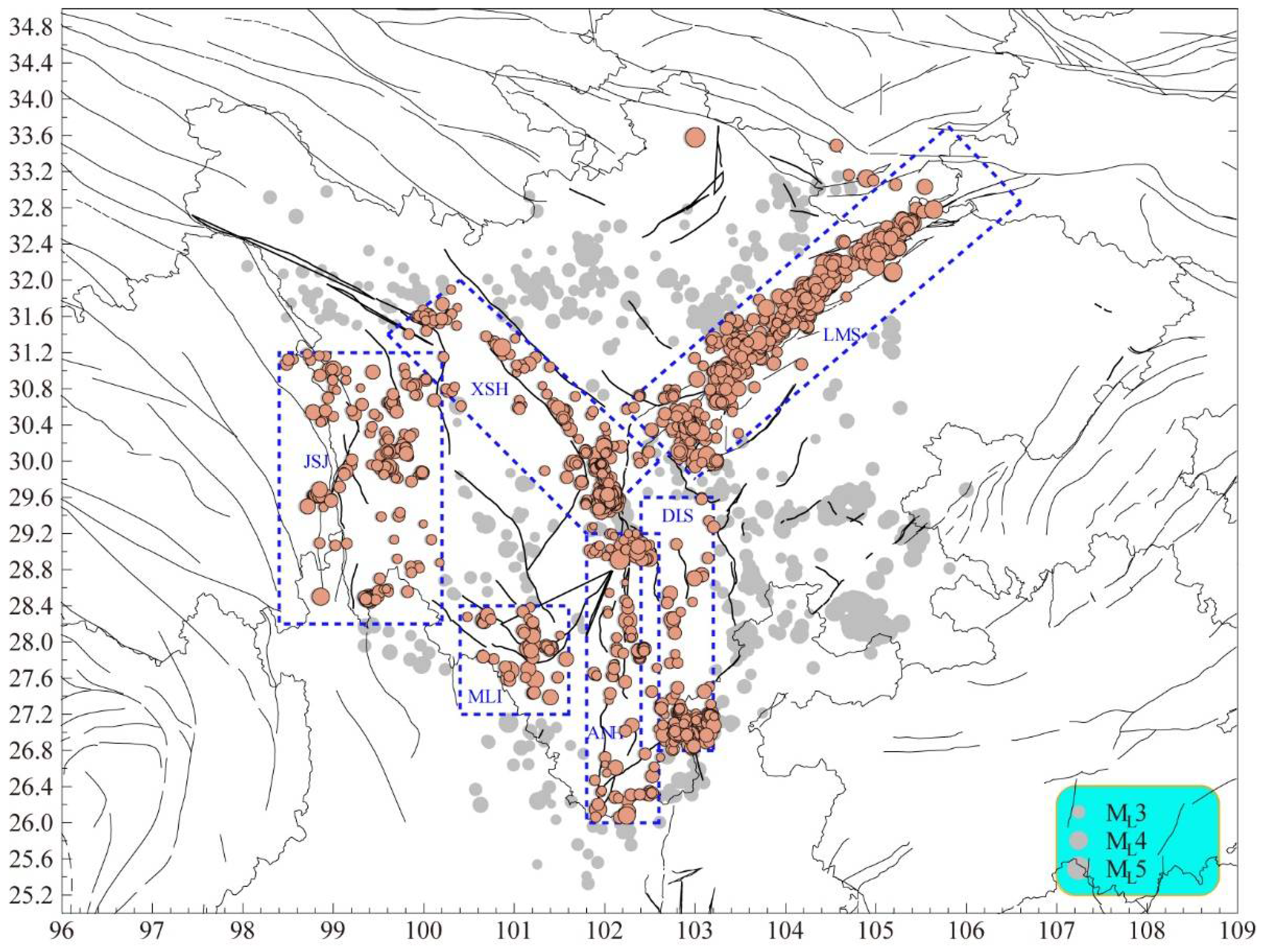
Figure 2.
Moment magnitude versus source scale (m).
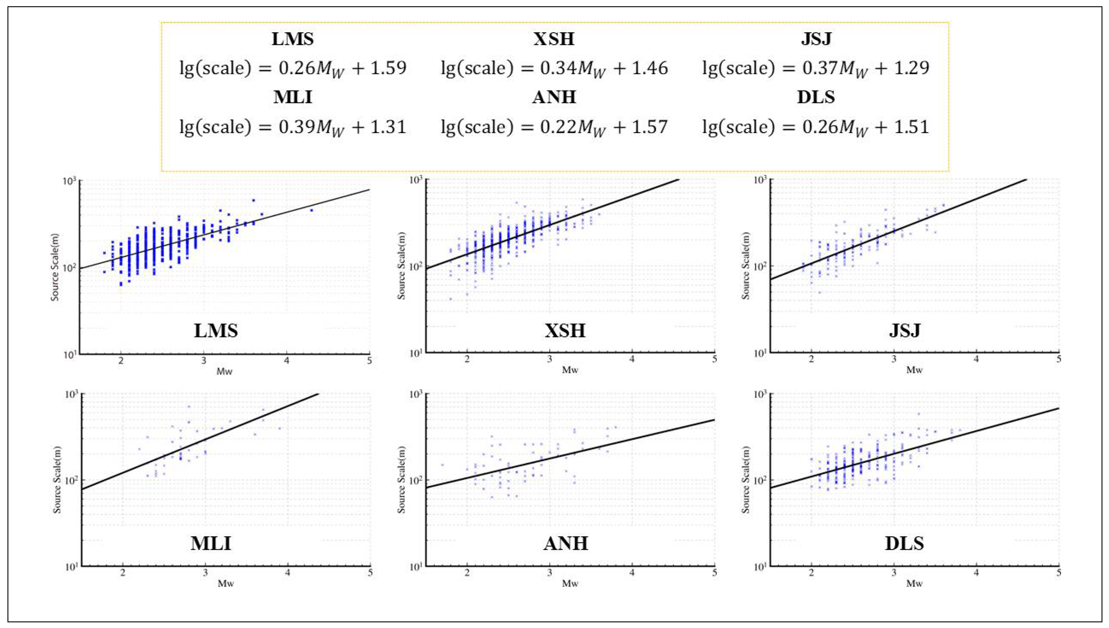
Figure 3.
Moment magnitude versus local magnitude .
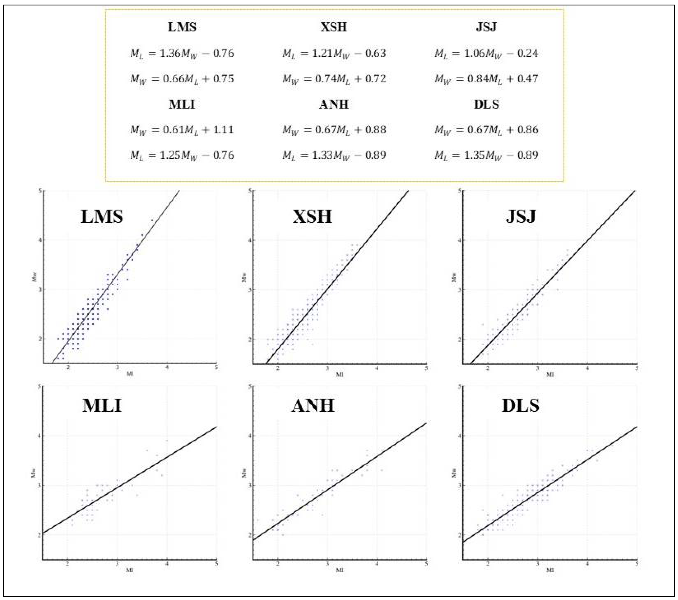
Figure 4.
Seismic moment versus local magnitude .
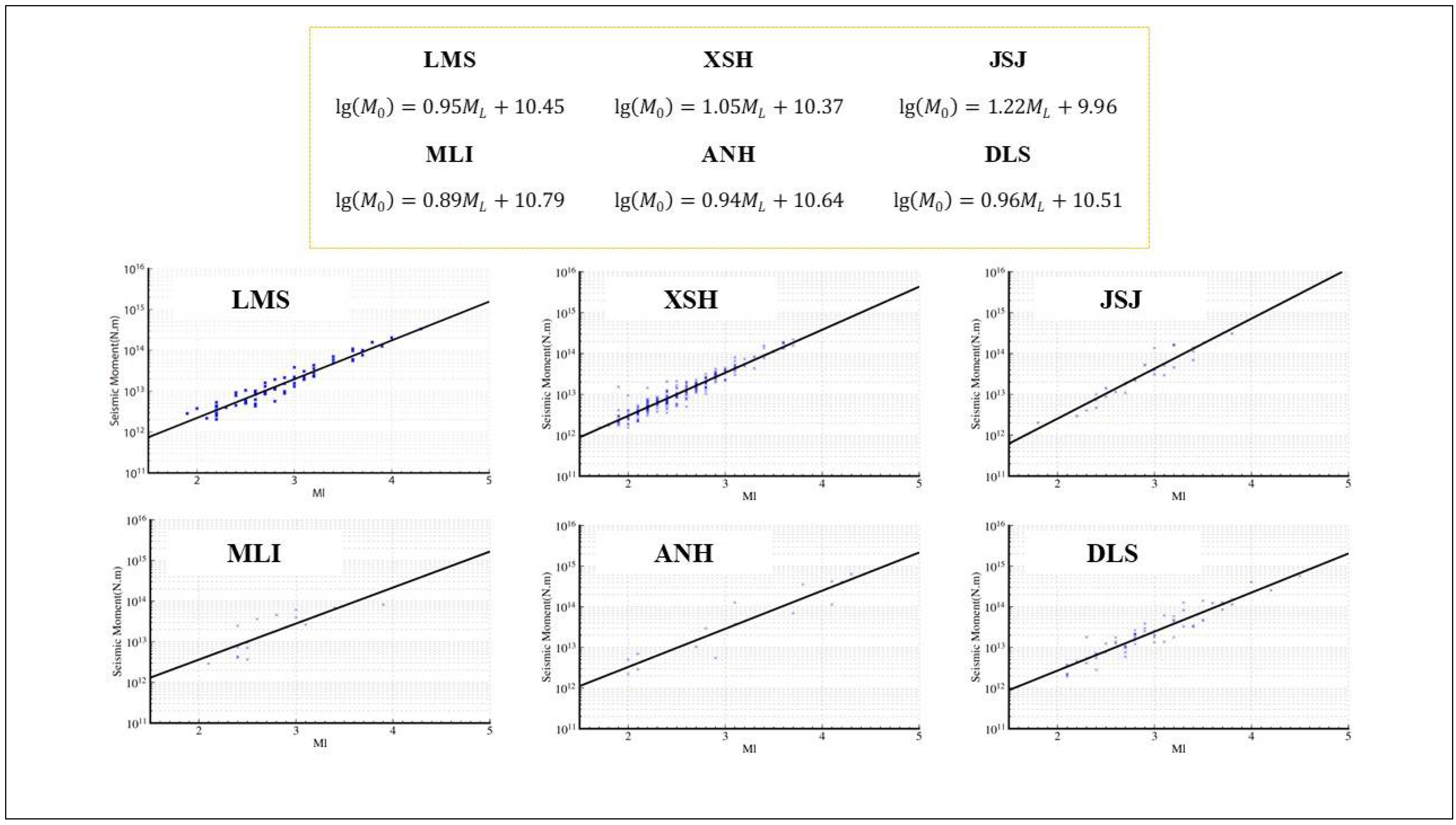
Figure 5.
Plot of seismic moment and source radius with the lines of constant stress drop in six tectonic zones.
Figure 5.
Plot of seismic moment and source radius with the lines of constant stress drop in six tectonic zones.
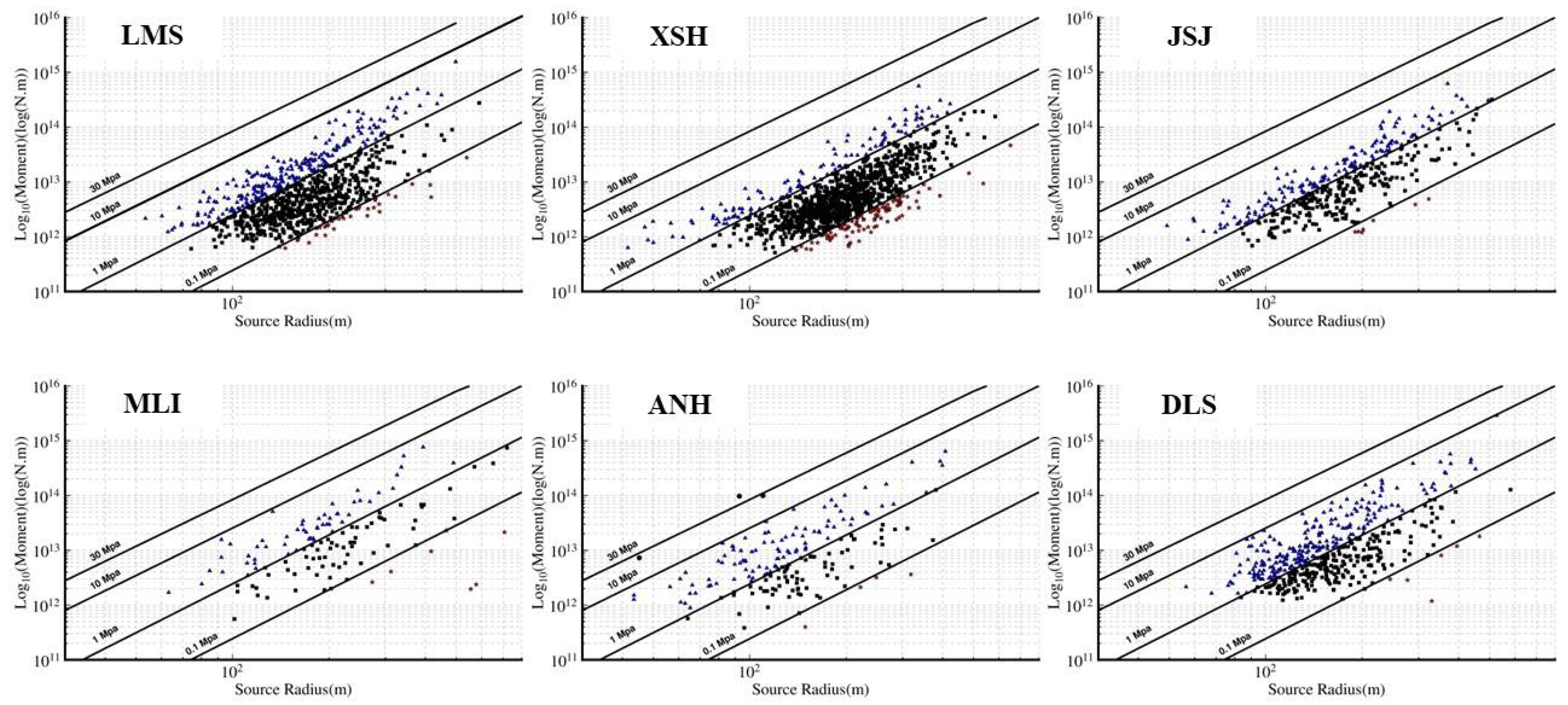
Figure 6.
The mean stress drop under different magnitudes rage in six tectonic zones. Blue hollow circle represents stress drop, yellow solid square represents the mean stress drop under different magnitudes.
Figure 6.
The mean stress drop under different magnitudes rage in six tectonic zones. Blue hollow circle represents stress drop, yellow solid square represents the mean stress drop under different magnitudes.
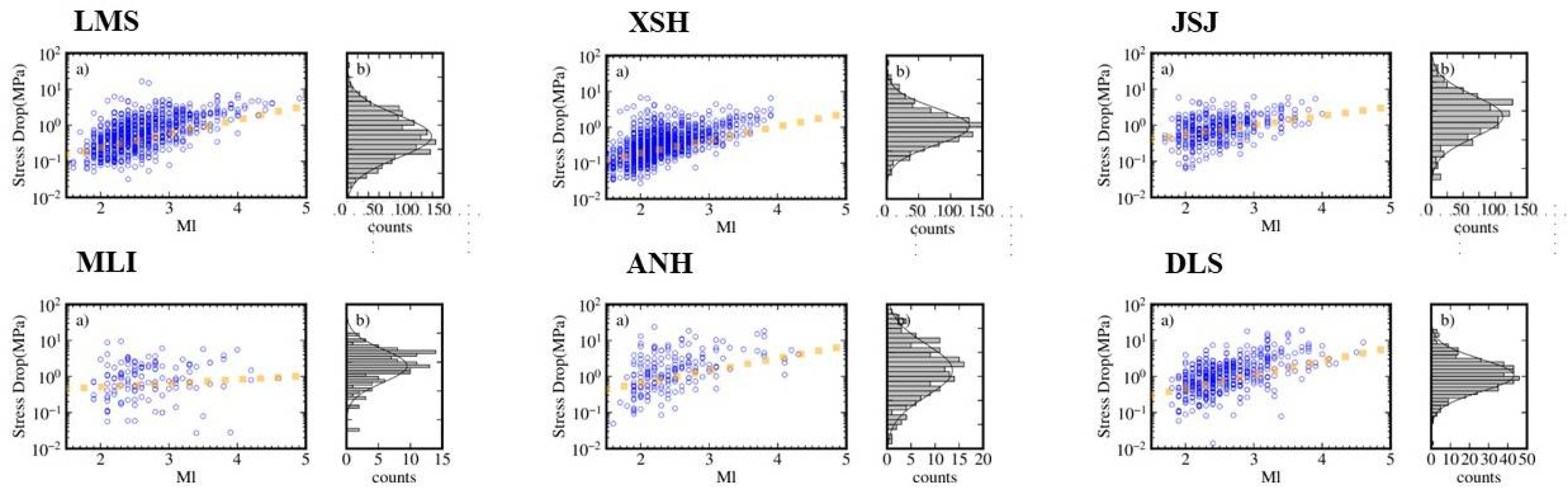
Figure 7.
Map view of stress drops for individual earthquakes in six tectonic zones. JSJ, Jinshajinag fault zone; LMS, Longmenshan fault zone; ANH, Anninghe-Zemuhe fault zone; XSH, Xianshuihe fault zone; MLI, Muli-Yanyuan fault zone; DLS, Daliangshan fault zone.
Figure 7.
Map view of stress drops for individual earthquakes in six tectonic zones. JSJ, Jinshajinag fault zone; LMS, Longmenshan fault zone; ANH, Anninghe-Zemuhe fault zone; XSH, Xianshuihe fault zone; MLI, Muli-Yanyuan fault zone; DLS, Daliangshan fault zone.
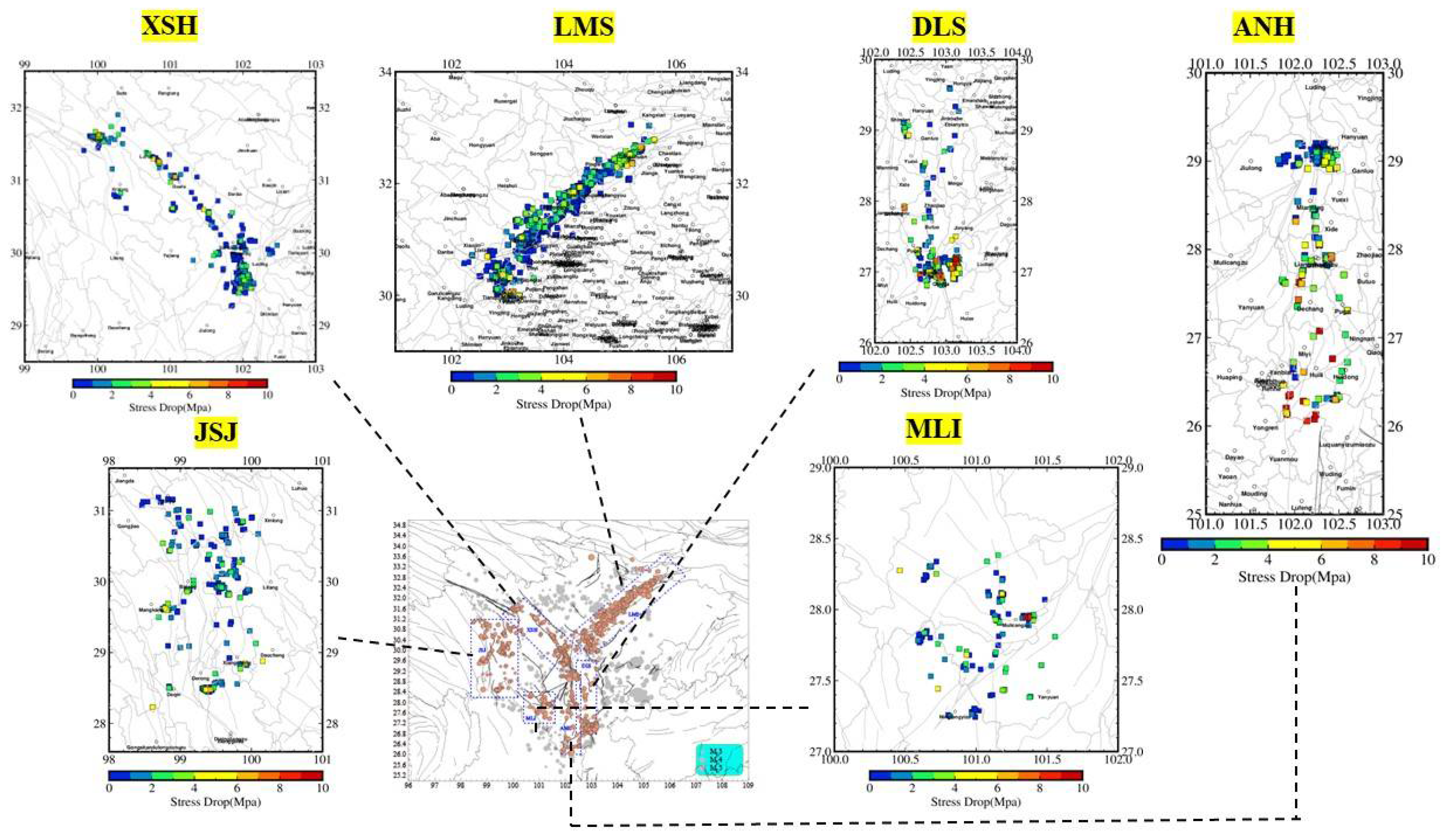
Figure 8.
Stress drops variations as a function of depth in LMS. (a) Stress drop distributed along the fracture trend. (b) Variation of stress drop with depth over time domain. (c) Variation of stress drop with depth after interpolation along strike. (d) Variation of stress drop with depth after Delaunay triangulations interpolation of the whole area in LMS. (e) The triangular plane of Delaunay triangulations interpolation.
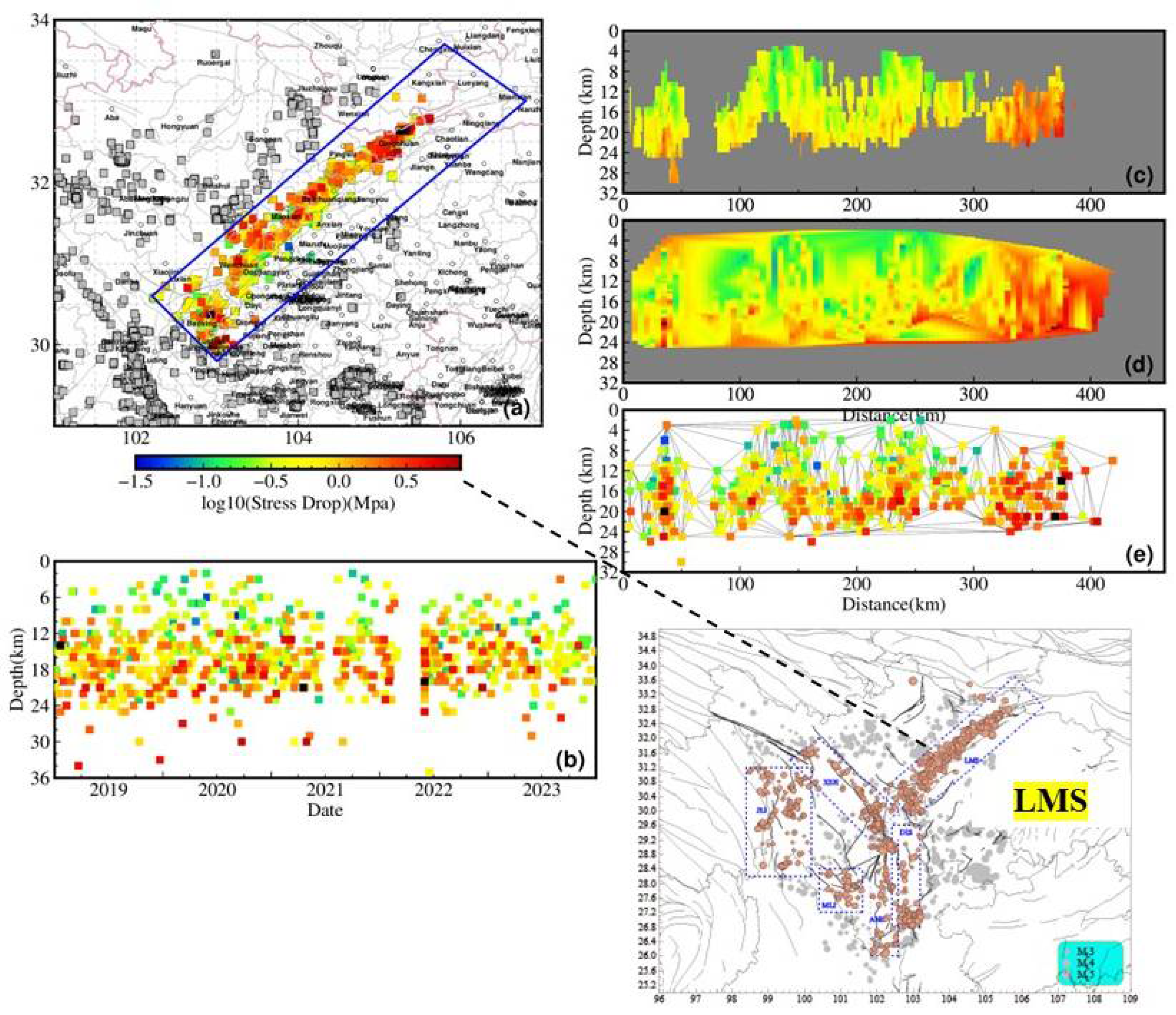
Figure 9.
Stress drops variations from 2013 to 2018. (a) Stress drop distributed along the fracture trend from 2013 to 2018. (b) Variation of stress drop with depth after interpolation along strike. (c) Variation of stress drop with depth after nearneighbor interpolation of the whole area in LMS. (d) Variation of stress drop with depth over time domain.
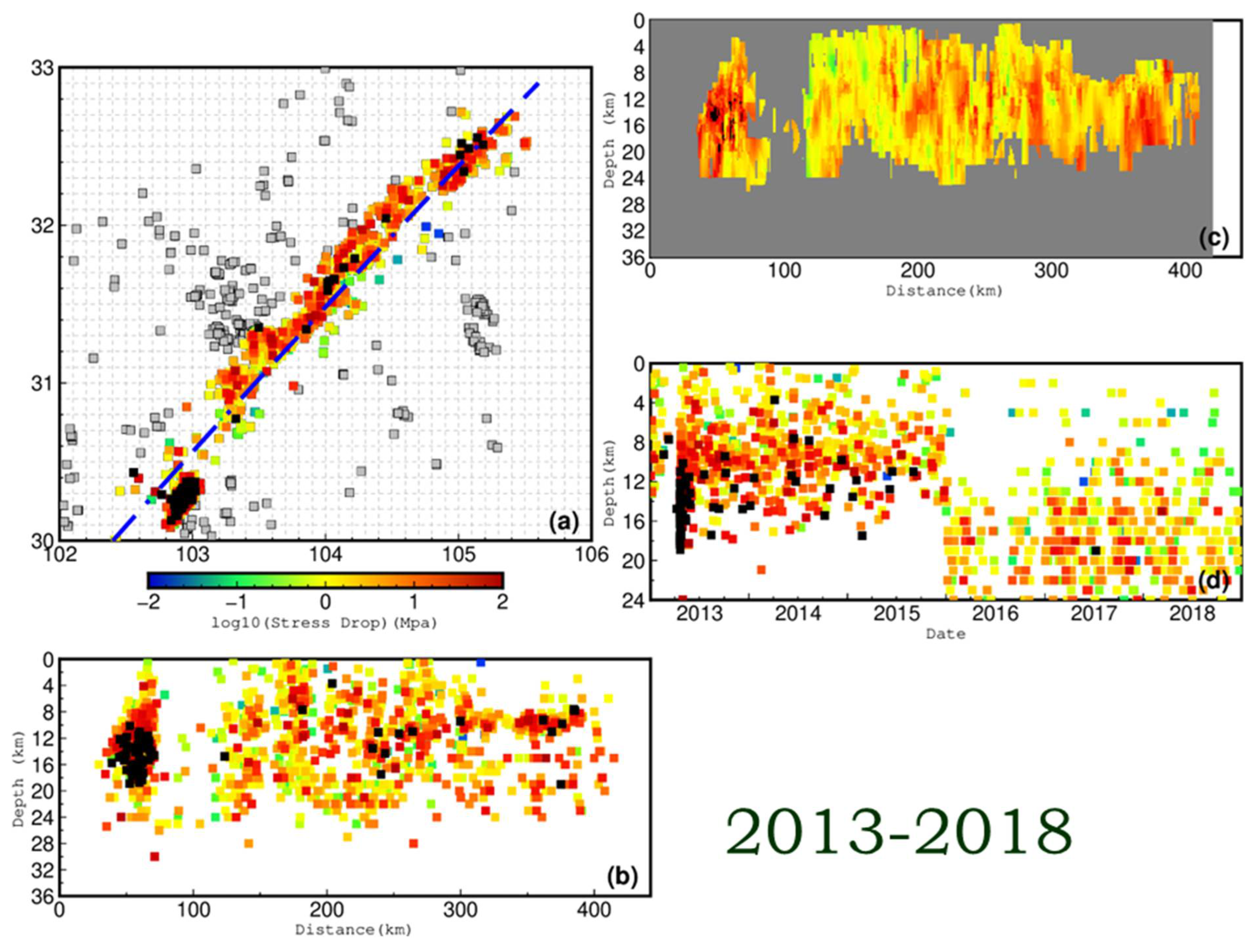
Figure 10.
Stress drops variations from 2019 to 2023. (a) Stress drop distributed along the fracture trend from 2019 to 2023. (b) Variation of stress drop with depth after interpolation along strike. (c) Variation of stress drop with depth after nearneighbor interpolation of the whole area in LMS. (d) Variation of stress drop with depth over time domain.
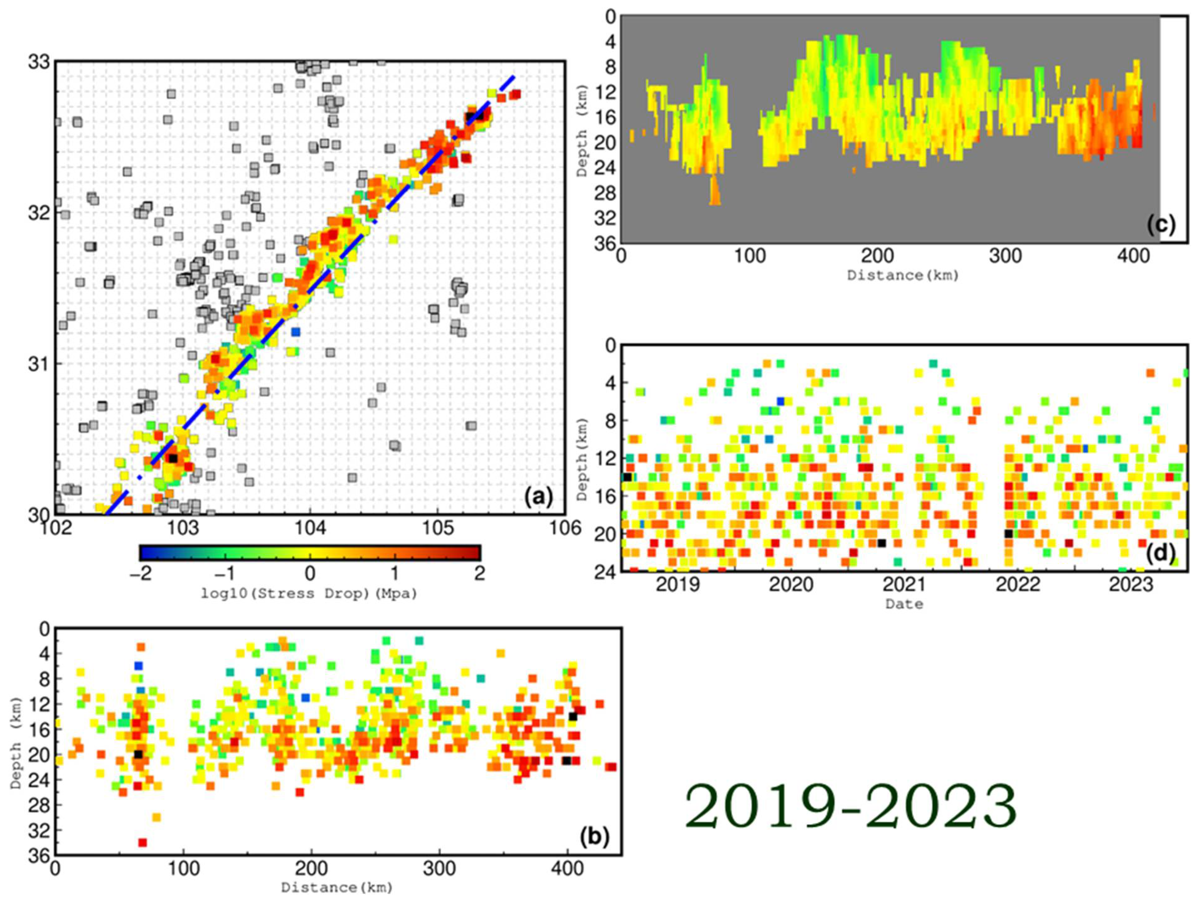

Table 1.
Scaling relations of seismic source parameters in six tectonic zones.
| LMS | XSH | JSJ |
|---|---|---|
| MLI | ANH | DLS |
Table 2.
The median stress drop varies with magnitude in six tectonic zones.
| LMS | XSH | JSJ | |||
|---|---|---|---|---|---|
| median | median | median | |||
| 2.0 | 0.32 | 2.0 | 0.35 | 2.0 | 0.65 |
| 3.0 | 1.41 | 3.0 | 0.85 | 3.0 | 1.58 |
| 3.5 | 1.73 | 3.5 | 1.38 | 3.5 | 3.72 |
| 4.0 | 3.11 | 4.0 | 3.48 | 4.0 | 5.4 |
| MLI | ANH | DLS | |||
| median | median | median | |||
| 2.0 | 0.44 | 2.0 | 0.82 | 2.0 | 0.81 |
| 3.0 | 0.78 | 3.0 | 1.70 | 3.0 | 2.55 |
| 3.5 | 2.9 | 3.5 | 5.65 | 3.5 | 3.61 |
| 4.0 | 5.4 | 4.0 | 9.82 | 4.0 | 5.60 |
Disclaimer/Publisher’s Note: The statements, opinions and data contained in all publications are solely those of the individual author(s) and contributor(s) and not of MDPI and/or the editor(s). MDPI and/or the editor(s) disclaim responsibility for any injury to people or property resulting from any ideas, methods, instructions or products referred to in the content. |
© 2024 by the authors. Licensee MDPI, Basel, Switzerland. This article is an open access article distributed under the terms and conditions of the Creative Commons Attribution (CC BY) license (https://creativecommons.org/licenses/by/4.0/).
Copyright: This open access article is published under a Creative Commons CC BY 4.0 license, which permit the free download, distribution, and reuse, provided that the author and preprint are cited in any reuse.
Submitted:
20 June 2024
Posted:
21 June 2024
You are already at the latest version
Alerts
This version is not peer-reviewed
Submitted:
20 June 2024
Posted:
21 June 2024
You are already at the latest version
Alerts
Abstract
Numerous investigations have suggested that seismic source parameters and properties of the surrounding medium harbor valuable information regarding alterations in stress fields and medium properties at the focal depth. Monitoring the spatial and temporal evolution of these parameters can yield insights into variations in stress fields or medium properties within the seismogenic zone, offering a critical avenue to overcome the Earth's inaccessible nature. In recent years, modern seismic parameters such as seismic moment, focal mechanism solution, source stress drop, corner frequency, radiated seismic energy, rupture radius, and apparent stress have been increasingly used to characterize source characteristics. The Sichuan region is situated on the southeastern edge of the Qinghai-Tibet Plateau and is known for its strong eastward extrusion and structural deformation. The main fault zones in the area include the Xianshuihe Fault, Anninghe Zemuhe Fault, and Longmenshan Fault. This paper estimates source parameters of small to medium-sized earthquakes (ML 1.5-5.2) in the main fault zones and adjacent areas in Sichuan. A total of 4,310 earthquake stress drop measurements from 2019 to 2023 were analyzed to create a stress distribution image along the fault. This earthquake parameters training catalog provides insight into how coseismic stresses change and their relationship with other geophysical factors, as well as their spatial and temporal evolution.
Keywords:
Subject: Environmental and Earth Sciences - Geophysics and Geology
1. Introduction
The earthquake process involves two fundamental interrelated links: the tectonic background and the seismogenic environment. The tectonic background refers to the large-scale dynamic energy required for earthquake occurrence, while the seismogenic environment pertains to local conditions under which strong earthquakes occur. It depends on the physical properties of the medium, tectonic activity, and stress state of the location where the earthquake occurs [1,2].
Earthquakes are the result of sudden instability and rupture caused by the continuous accumulation of strain in discontinuous deformation areas, ultimately reaching the limit state under regional tectonic stress provided by the tectonic background [3]. Non-continuous structural areas are often where strain is most easily accumulated and structural deformation is strongest, making them favorable locations for strong earthquake development.
Experiments in Structural Physics [4,5,6,7,8] have indicated that main-aftershock type earthquakes predominantly occur in homogeneous medium environments. In contrast, fore-main-aftershock type earthquakes and swarm type earthquakes tend to occur in complex tectonic environments. Analysis of the modern tectonic stress field and intense seismic activity suggests a significant correlation between stress distribution and the occurrence as well as recurrence of earthquakes.
On the one hand, regions experiencing strong and complex tectonic stress, as well as changes in the direction and type of stress, are more susceptible to powerful earthquakes. It is common for large earthquakes to occur in areas where there is a relatively high accumulation of stress within active fault zones or in sections where fault zones are relatively locked; On the contrary, the local stress variation area in a uniform stress field background is an area where strong seismic activity is relatively concentrated. Under specific conditions, even a small stress variation of 0.1 bar magnitude can significantly impact seismic activity. Research conducted by Xu et al. [9] has indicated that faults capable of generating high magnitude earthquakes often exhibit low b-values and high stress anomaly segments. Additionally, their pre-earthquake locking characteristics are essential prerequisites for stress or strain accumulation and the occurrence of high magnitude earthquakes.\
The type of earthquake sequence is also influenced by the overall level of stress. Isolation-type earthquakes typically occur under conditions of high prestress and/or low rupture strength, while front-main-residual type earthquake sequences tend to occur under conditions of medium prestress and/or medium rupture strength. Additionally, swarm-type earthquake sequences are associated with low prestress and/or high rupture strength conditions [10].
When utilizing seismological methods to assess the risk of significant earthquakes within a research area, the M6.0 earthquake in Parkfield in 2004 serves as a typical illustration. Allmann and Shearer [11] emphasized that enhanced stress is often observed in fault areas prior to a strong earthquake, and there is a substantial decrease in regional stress drop following the event. Hardebeck and Aron [12] proposed that regions with higher strength or subjected to greater external shear stress are more likely to exhibit higher source stress drop, and areas with concentrated distribution of high stress drop may serve as potential nucleation sites for moderate to large magnitude earthquakes.
In addition, stress intensity provides crucial information regarding the potential energy release of earthquakes, while stress characteristics offer insights into the possible types of earthquakes. Tensile stress indicates regions under tension and suggests a potential occurrence of earthquakes on normal faults; compressive stress points to areas under compression, indicating a likelihood of earthquakes on reverse faults; neutral stress implies a strike-slip earthquake. Therefore, conducting quantitative research on the state of stress and its variations in the deep seismogenic layer is an essential method for investigating the issue of predicting strong earthquakes.
Due to challenges such as the difficulty in accessing the Earth’s interior and the infrequency of large earthquakes, direct measurement of stress and intensity in the deep crust remains elusive for humans. Numerous studies have indicated that earthquake source parameters and medium properties contain valuable information about changes in stress fields and medium properties at the focal depth. Monitoring the spatio-temporal evolution of these parameters can provide insights into changes in stress fields or medium properties within the seismogenic zone, offering an important means to overcome the Earth’s inaccessibility.
Scientists use various physical parameters to describe an earthquake, and these parameters that depict the mechanical characteristics of the source are known as the source mechanical parameters, abbreviated as the source parameters. Traditional “earthquake statistics” typically only focus on the “time, space, and intensity” sequence of earthquakes. In recent years, modern seismic parameters such as seismic moment, focal mechanism solution, source stress drop, corner frequency, radiated seismic energy, rupture radius, and apparent stress have been increasingly utilized to characterize source characteristics.
A plethora of earthquake examples indicate that the physical properties of large earthquakes differ from those of small and moderate earthquakes in actual earthquake processes. The source characteristics of the former largely reflect the seismic tectonic background, stress mode of the source, and result in a larger rupture area, while small and moderate earthquakes more so reflect non-uniform changes in stress state within a smaller area. The study of source parameters of small and moderate earthquakes not only serves as the basis for exploring the source process of large earthquakes but also provides new insights for studying regional stress states and evaluating potential earthquake magnitudes.
The Sichuan region (Figure 1) is situated on the southeastern edge of the Qinghai-Tibet Plateau and is known for its strong eastward extrusion and structural deformation. The main fault zones in the area include the Xianshuihe Fault [13], Anninghe Zemuhe Fault, and Longmenshan Fault. Over an extended period of geological evolution, this research region has undergone complex structural deformation, leading to a diverse seismic activity behavior within a dynamic environment.
The gray circle represents the background seismic event, while the orange circle signifies the seismic event that is involved in the calculation of source parameters. Additionally, the blue box indicates the six main tectonic areas in Sichuan.
Sichuan is an important area for strong earthquake monitoring in China, with at least 15 earthquakes of magnitude ≥ 7 occurring in just over 200 years. There are significant differences in the seismic activity characteristics of the regional main and secondary faults. Strong earthquakes of magnitude ≥7 mostly occur on the Xianshuihe fault. No earthquakes of magnitude ≥ 7 have occurred on the Anninghe fault since 1536, the Zemuhe fault since 1850, the Jinshajiang fault since 1870, or the Litang fault since 1948. Therefore, understanding the changes in stress state among different faults within this research area has become a focus of attention.
To understand the current stress distribution characteristics of the primary active faults in the region and identify sections where relatively high stress accumulation is occurring, this paper estimates the source parameters of small and medium-sized earthquakes (ML 1.5-5.2) in the main fault zones and adjacent areas in Sichuan. A total of 4,310 measurements of earthquake stress drops during the 5-year period from 2019 through 2023 are analyzed to draw a stress distribution image along the fault. The study discusses the stress distribution characteristics on major faults, variations of seismic stress drop with location, and correlations between stress-strain loading and regional deformation dynamic processes based on geometric structure, activity habits, and temporal spatial distribution of modern seismic activity in different sections of the region. This earthquake parameters training catalog provides an opportunity to understand how coseismic stresses change and how other geophysical factors relate to the distribution of stress drop as well as its evolution in space and time.
2. Main Fault Zones and Their Activity
2.1. Longmenshan Fault Zone (LMS)
The Longmenshan fault zone is located on the eastern edge of the Qinghai Tibet Plateau, at the junction of the Bayankala block and the Yangtze block. The Longmenshan fault zone has four main faults developing from northwest to southeast: the Maoxian Wenchuan Fault (Houshan Fault), the Beichuan Yingxiu Fault (Central Fault), the Jiangyou Guanxian Fault (Qianshan Fault), and the Guangyuan Dayi Fault (Hidden Fault in front of the Mountain). The dextral strike slip rate (<1mm/a) and vertical slip rate (<1mm/a) of the Longmenshan fault zone are both very small [14,15], and multiple periods of sliding have occurred. The secondary fault exhibits long-term creep deformation characteristics [16,17].
The 2008 Wenchuan 8.0 earthquake occurred on the Longmenshan Fault zone, causing both the Beichuan Yingxiu Fault (Central Fault) and the Jiangyou Guanxian Fault (Qianshan Fault) to rupture simultaneously. The surface rupture zone of the central fault is about 240km long, mainly characterized by reverse fault displacement, and also has a right lateral strike slip component. The surface rupture of the Qianshan Fault is about 72km long, which is a typical reverse fault displacement property. The 2013 Lushan 7.0 earthquake occurred in the southern section of the Longmenshan Fault zone, which was a blind reverse fault type earthquake. No structurally significant fractures were found on the surface.
2.2. Xianshuihe Fault (XSH)
The Xianshuihe fault of western Sichuan Province, China, is one of the world’s most active faults, can be divided into two segments of different structural styles, jointing at the pull-apart area of Huiyuan Monastery. The northwestern segment has a relatively simple geometric structure. While the southeastern segment exhibits a complex structure composed of several branches. In the southern part of Huiyuansi, the fault is divided into three secondary parts as Yalahe fault, Selaha fault, and Zheduotang fault. To the south of Kangding, it is manifested as a main fault with only local branching phenomenon, known as the Moxi fault.
The Xianshuihe fault is a highly active strike-slip fault system. Since earthquake records began in 1700, the Xianshuihe fault has experienced eight M>7.0 earthquakes, accounting for about half of the total earthquakes of the same magnitude in the entire western Sichuan region. The surface rupture zone of the earthquake almost covers various sections of the entire fault.
2.3. Jinshajinag Fault (JSJ)
The Jinshajiang fault is composed of multiple SN direction arc-shaped secondary reverse faults and the NNE trending Batang fault. There is almost no seismic activity on the arc-shaped secondary fault. Moderate historical earthquakes have occurred on the west segment of the Batang Fault, such as the earthquakes of 1989 M6.7, 2006 M 5.0, M 5.4 and M 5.6 in Balongda. From the perspective of active structure, the arc-shaped secondary reverse fault is a complex fracture zone composed of numerous small faults and fault combinations, which is not easy to concentrate stress. Seen from Google earth images, the Batang fault has a clear geomorphic expression, however, geometry and late Quaternary slip-rate are still unknown.
2.4. Muli-Yanyuan Fault (MLI)
The active fault system of this unit is mainly composed of the NE oriented Lijiang Xiaojinhe fault zone and secondary faults parallel to it, in addition to the Muli Arc Fault, Zhongdian-Daju Fault, and Ninglang Fault. These main and secondary active faults intersect and intersect locally, resulting in frequent seismic activity in this unit both historically and today. Among them, the Lijiang-Xiaojinhe Fault cuts through the Research diamond block and divides it into two parts: the northwest Sichuan secondary block and the central Yunnan secondary block. The Ninglang-Yanyuan and Muli areas are located at the junction of the south and north secondary blocks.
2.5. Anninghe-Zemuhe Fault Zone (ANH)
The Anninghe Fault zone is located on the axis of the Kangdian earth axis, starting from Shimian in the north and extending through Xichang to the Huili area. It generally runs in an NS direction and is mainly characterized by sinistral strike slip movement. In history, this area may have occurred 1470 AD earthquake.The Mianning-Xichang area in the southern section of the Anninghe fault was the main rupture part of the M 7½ in 1536.But since the M 63/4 earthquake in south of Mianning in 1952, there have been no larger earthquakes on the Anninghe Fault. A modern seismic gap gradually formed with the Liziping-Xichang section as the core, with the background of the first kind seismic gap.
The northern end of the Zemuhe fault is connected to the Anninghe fault, and the southern end is connected to the Xiaojiang fault. It extends from Xichang through Puge and Ningnan to Qiaojia, with an overall trend of 330°. There have been M 7 earthquakes in 814 AD and M 7½ earthquakes in 1850. The most recent moderate earthquake was the Xichang M5.1 earthquake on October 31, 2018. The Zemuhe fault is mainly characterized by sinistral strike slip movement, with a sinistral strike slip rate of about 6.4 ± 0.6 mm/a in the Holocene [13], accompanied by a normal fault dip slip component between Xichang and Puge [18]. In the southwest of Qiaojia, the southernmost fault of the Zemuhe fault zone deviates towards the south southwest direction.
2.6. Daliangshan Fault (DLS)
The Daliangshan fault is left-lateral strike-slip fault approximately 250 km long. The Daliangshan fault has a complex fault geometry characterized, and mainly composed of four secondary faults, including the Yuexi Fault, Puxiong Fault, Butuo Fault, and Jiaotong River Fault. The historic earthquake record is no M≥6.0 strong earthquakes on the Daliangshan fault. But seismic and geological studies have confirmed that the fault has experienced prehistoric strong earthquakes and has the structural conditions for the breeding and occurrence of strong earthquakes [19,20,21].
3. Database
The estimation of source parameters is of great significance to reveal whether the rupture mechanism of large and small earthquakes has the same physical process, and to apply source parameters to the study of earthquake prediction and to understand the physical properties of earthquakes. The effective stress, stress drop, and source size can be estimated by comparing the measured seismic spectrum with the theoretical spectrum [22]. Static stress drop is the simplest method to measure the overall reduction in shear stress caused by sliding of fracture zones [23]. It is the difference between the average shear stress on the fault zone before and after the earthquake, and represents the stress released on the fault plane during the earthquake. Assuming that the static initial shear stress on the fault plane before the earthquake is and the final shear stress on the fault plane after the earthquake is , the static stress is reduced by
The average stress is
Since the stress drop of a real earthquake varies throughout the fault zone, the overall static stress drop is the sliding weighted average of the spatially variable stress drop [23].
The corresponding dynamic stress drop is more complex because the space-time history of stress drop can be quite variable. Any individual part of the fault plane may have a variable stress drop during sliding. Due to the impossibility of reliably inverting seismic waves to determine the complete spatiotemporal process of dynamic stress drop, the simplest viewpoint is that the dynamic stress drop is constant on the spatiotemporal window of fault sliding.
When the earthquake rupture begins to expand, the stress at this point gradually increases to the horizontal stress that the rock can withstand, the rupture occurs at this point. For the region without rupture, is the shear fracture strength of the material or rock. To have broken down, for the two discs of the fault and squeezed together by static friction stress, is the maximum static friction stress. When sliding occurs, the stress decreases from to the dynamic friction stress , and the dynamic friction stress remains unchanged during sliding. As the rupture process on the whole fault surface stops, the stress transitions from the dynamic friction stress to the final stress .
The shear rupture strength, or the difference between the maximum static friction stress and the dynamic friction stress , is called the effective stress
In the Brune [22] disk model, assuming that shear failure occurs simultaneously and , the effective stress is the dynamic stress drop
Seismologists generally use simple constant stress drop model to estimate the seismic stress drop. In the method of estimating stress drop using the scaling relation [24,25], regardless of the details of fault geometry and slip distribution, assuming that the earthquake rupture process is a linear elastic process in semi-infinite space. The basic formula for stress drop is as follows
where is the average displacement that occurs on a fault of length L at the time of the earthquake, is the elastic shear modulus. Since seismic moment (M0) for most large earthquakes can be reliably determined from seismic waves, rewrite the above equation as:
where is the fault shape parameter,, refers to the length of the fault, and refers to the width of the fault. Then
or
is the fault area.From formula (7) and (8), we need three quantities to calculate stress drop: a measurement of the seismic moment (), some estimate of the fault area (A), and then some appropriate choice for the characteristic fault dimension ().
In practice, it is very difficult to determine the characteristics of seismic source rupture. It is common to assume a theoretical rupture model to calculate the stress drop, then different geometric coefficients and fault feature length are taken according to the calculation model [25]. For large earthquakes, the rupture scale in the direction of the fault can be tens to hundreds of kilometers, the depth direction is limited by the focal depth, and generally adopt × rectangular model, taking , then the stress drop is expressed as
For the infinite dip-slip fault model,
is the Lame coefficient.
For small magnitude earthquakes, Brune’s [22] disk rupture model is often used, which assumes that earthquake rupture occurs on a circular fault plane with uniform stress drop and constant rupture velocity. Usually c=7π/16, take the disc radius , stress drop is expressed as
For the acquisition of the rupture radius , the source rupture process can be retrieved from the far-field seismic records in seismology, by the frequency domain of corner frequency indirect access to the source physical dimension information [26,27], expressed as
is the shear velocity near the source.
Then formula (11) is rewritten as
is a constant, depending on the type of model used to correlate the relationship between the corner frequency and the focal rupture radius . In Brune [22] model, ; In the Madariaga [28] model, [29,30]; In Sato and Hirasawa [31], depends on the source rupture velocity [32].
The obtained by equation (13) is proportional to the cube of , so the stress drop is very sensitive to the error of . Even if the fault model is close to the actual fault, the small observation error of will reduce the reliability of , which is also the limitation of the traditional seismological method to give the seismic stress value.
4. Results
4.1. Scaling Relationships of Earthquake Source Parameters
The relationships between earthquake source parameters like seismic moment ,or magnitude , moment magnitude ,stress drop , corner frequency , and source scale r ,are termed as scaling relations [33,34]. The self-similar of earthquakes is manifested on many scales, which means that stress drops remain constant over a large range of earthquake magnitudes, and fault sliding systematically increases with the fracture area. However, other studies have emphasized the possible self-similarity bias at regional and global scales, indicating that stress reduction may vary with earthquake magnitude and different regions [35,36].
Here, we try to unravel measurement uncertainty and potential physical differences in earthquake source processes by analyzing source spectra of more than 4,310 micro-earthquakes ranging from ML 1.5 to ML 5.2 in the 5-yr time period from 2019 through 2023. Analyzing a large number of small-magnitude earthquakes enables us to better resolve statistically significant variations in source parameters, such as stress drops, even if scatter is high. We analyze seismograms, including those of numerous small earthquakes, to calculate the scaling relations of seismic source parameters in six tectonic zones (Table 1).
The moment magnitude reflects the magnitude of deformation and is an absolute mechanical scale for describing earthquake size which does not cause saturation problems. So, it is the best physical quantity for measuring earthquake size currently. By assuming specific models of fault geometry and fracture dynamics, the seismic moment of the source spectrum can be used to determine the size of the fracture. Here in six tectonic zones, as the moment magnitude increases, the source scale increases linearly (Figure 2).
Both local magnitude and seismic moment or equivalently moment magnitude are measures of basic properties of the earthquake source: is proportional to the maximum of the moment-rate function, whereas is proportional to its integral. Thus, theoretical considerations and empirical regressions show that, the values of and should be the same for special earthquakes caused by similar source processes. However, the observed data do not match the ideal situation.
The observation that the theoretical 1:1 relationship breaks down in empirical relationships was explored by Hanks and Boore [37]. Ben-Zion and Zhu [38] proposed that an alternative cause of the deviation from 1:1 scaling could result from non-self-similarity of earthquake sources. For small events the heterogeneity of a tectonic stress field may lead to slip that does not grow substantially with rupture dimension, whereas for larger events the effect of small-scale stress heterogeneities is smoothed out. That means the evolution between the two extremes of small and large events could lead to the observed polynomial form of - scaling.
In our research,a difference was also observed between and . We performed linear regressions for versus in different areas (Figure 3), and found that for small magnitude events, this 1:1 relationship is ineffective. However,from these data we observed systematic deviations of relative to , simultaneously fitting the linear scaling relationship between and . The determination of for small events is desirable to obtain robust a and b values in a recurrence relationship and the magnitude of completeness of the earthquake catalogue.
To improve our understanding of these differences between and , some studies suggest that it can be attributed to the variation in the physical properties, as attenuation and scattering along the path, pore fluid pressure, temperature, and related changes in normal stress, interface morphology, and material properties [39,40].
4.2. Stress Drops Training Catalog
Stress drop is a basic parameter that describes the characteristics of the source scale. Earthquake stress drop is defined as the difference in average shear stress on the fault plane before and after an earthquake, representing the stress released on the fault plane during the earthquake. This study aims to investigate the spatio-temporal distribution of static stress drop values of the six faults rupture seismic sequence in Sichuan. We observe that the vast majority of earthquakes have stress drop between 0.1 and 1 MPa, some earthquakes are between 1 MPa and 10MPa, a few earthquakes have stress drop less than 0.1MPa, only few events are greater than 10MPa (Figure 5). We find several anomalous events with unusually high or low stress drops in the small earthquake parameters training catalog. Individual event stress drops show some scatter. Previous studies [11] have suggested that this divergence presumably caused by inherent uncertainty in the computation method and a combination of other effects, including uncertainty in corner frequency estimation, incomplete averaging of radiation pattern effects,heterogeneities in the physical properties of faults and simplified assumptions about the source model.
Given these sources of uncertainty, it should not be assumed that a single stress drop estimate for a particular event can be generalized to an entire region. Analyzing a large number of small-magnitude earthquakes enables us to better resolve statistically significant variations in stress drops even if scatter is high. In our study, the stress drop was calculated using the same analytical methods and the same source model assumptions for each earthquake in separate tectonic area, so their relative values should be meaningful. We therefore focus on the properties of the data set to obtain statistically significant differences in stress drop to study the relative stress drop between events generated under different tectonic conditions in Sichuan, although the absolute value of the stress drop remains somewhat model dependent. To detect a possible dependence in the highly scattered values, we classify seismic events in different tectonic zones. This classification of events allows us to calculate and investigate median stress drops for each tectonic region. We apply a bootstrap method over 100 resamples for each tectonic region and estimate the median stress drops which represent averages of individual stress drops which are highly scattered. These are listed in Table 2 for each tectonic regime. It is interesting to note that the median stress drop varies with magnitude in different tectonic zones. For most regions, the distribution of stress drops shows a clear peak that allows us to derive meaningful statistics.
Recent observations have suggested that as earthquakes increase in magnitude, they radiate an increasingly large amount of energy [25,43], which implies that stress drop varies with magnitude. We also observed this phenomenon in this study. Although there are actual differences in the spatial patterns of stress drop with seismic moment in different faults (Figure 6), the overall stress drop value for small and medium earthquakes increases with the magnitude increase.
4.3. Spatial Variation of Stress Drops
The spatial distribution of stress drop values in a complex seismic sequence could support a more complete understanding of the earthquake rupture process and the evolution of seismic sequences. It could also highlight areas where stress loading is focused, which would have implications for short and intermediate term seismic hazard estimates [11,29].
Figure 7 shows the individual stress drop estimates at the event locations. At first sight, we observe no obvious correlation with tectonic regime. However, we do observe areas with overall higher or lower average stress drop than their surrounding regions. A particularly striking feature is the region of low stress drop estimates along the XSH fault zone with average values below 2.78 MPa. Examples with higher-than-average stress drops are the ANH fault zone with values around 5.11 MPa and the region near Qiaojia in Yunnan province.
The LMS fault zone shows a very heterogeneous stress drop pattern. We observe an apparent variation along strike with lower stress drop values near the hypocenter of the great Wenchuan earthquake of 2008, and higher stress drops both to the northeast and to the southwest. However, because of the dense clustering of events in this region and a variation of tectonic regimes over short distances, we need to look at a finer regional scale in order to clearly see differences and possible correlations in LMS fault zone.
The stress drop also generally increases with depth [44]. Normal stress on faults increases with depth in the earth and has long been thought to be a potential factor influencing earthquake stress drops [45]. However, some studies have also interpreted the dependence of stress drop on focal depth as an observation illusion [46],which vary significantly along strike [47,48], and to depend on fault rheological and geometrical complexities [49].
We plot the stress drop distribution at a depth of 0-36km in six tectonic zones, and take the depth distribution of the stress drop on the LMS as an example to demonstrate. In order to effectively solve the color matching problem caused by the excessive range of data values, the stress drop data are drawn in Figure 8 after logarithmic selection. In LMS, the high stress drop values are distributed along the fracture trend and mainly occurred from 2019 to 2022. After interpolation along the central fault strike of Longmenshan fault and using the nearest neighbor algorithm to calculate the weighted average of grid points, it is found that stress drop estimates largely constant within the upper 9 km and show a sharp increase at 10km from 3 MPa to 10 MPa. After Delaunay triangulations interpolation [50,51,52,53] of the whole area, the data results show that the high stress drop events are concentrated in the depth range of 20-24km. Even though our study regions in LMS host some of the deepest seismicity in Sichuan, observations of stress drop as a function of depth show considerable variability and the systematic variation of stress drop with depth is not particularly obvious.
5. Discussion
Much research in recent years shows that the average difference in shear stress (static stress drop) on faults caused by earthquakes is usually between 0.1 MPa and 100 MPa [11,29,54,55,56]. In this paper we explore the small earthquake stress drop training catalog on the main faults in Sichuan, the stress drops are usually between 0.1 MPa and 10 MPa. It should be noted that there is considerable scatter in the stress drop estimates above about 30 MPa, which reflects large uncertainties in measuring corner frequencies that are near the 25-Hz upper-frequency limit of our analysis. Thus, these very high values should not be considered reliably resolved although they should be retained in computing median stress drops as they are almost certainly on the high side of the stress drop distribution [55,57,58].
5.1. Self-similar Earthquake Scaling
The source-scaling relationships, including whether stress drop is self-similar and magnitude-invariant [34] or obeys a more nuanced scaling relation. Self-similar earthquake scaling has been observed at many scales, which means that stress drops remain constant across a wide range of magnitudes and that fault slip increases systematically with rupture area [34,59,60]. However, an increase in stress drops with seismic moment would imply non-self-similar earthquake scaling and whether this occurs has been the subject of considerable debate [41,57]. Other studies have emphasized on regional and global scale possible deviation of self-similarity, suggests that stress drops may change with earthquake magnitude in different areas [36]. But source parameter estimates often exhibit a puzzling degree of scatter [57], and results from different methods are often inconsistent, even when using the same underlying data set.
In our study, we have observed a consistent trend of increasing stress drop with magnitude, indicating the presence of self-similarity rule. The same equivalent stress drop line (Figure 5) can traverse at different seismic scales (ordinate), while the fracture scale (abscissa) and seismic moment (ordinate) have the same slope as the stress drop line, which indicates that there is a self-similarity between the fracture scale and seismic moment, and the stress drop can be a constant at different magnitude scales.
It is important to note that the modeling assumptions can significantly impact the absolute values of stress drops, which may not accurately represent the true static stress drop of the earthquake rupture. Our focus in this study is on relative variations in stress drops, which were estimated consistently and can be interpreted as reflecting variations in high-frequency energy release. Higher and lower stress drops correspond to energetic and enervated events, respectively.
5.2. Spatio-Temporal Stress Drop Evolution
In addition to studies exploring systematic variations in stress drop with size, there have been continuous efforts to determine whether stress drop varies based on tectonic environment, faulting mechanism, or focal depth. Recent studies have identified spatial and temporal variations in stress drop in California [11,30,61], Japan [56,62,63], and New Zealand [64]. These papers suggest that spatial and temporal variations of stress drop have the potential to reveal heterogeneities and demonstrate more nuanced changes in the character of a stress field on a fault [12,65]. In this paper, the earthquake sequences are used for detailed studies of spatio-temporal variations in the stress state of the six main tectonic areas with different structural inheritance in Sichuan, to outline regions of alternating high and low stress drop. The relationship between stress drop and faulting regime could help to identify fault segments with relatively high stress accumulations, which generally indicate greater applied shear stresses or the presence of higher-strength materials [12].
From the spatial distribution (Figure 7), we observe that regions of high and low stress drop alternate on either side of the six main tectonic areas. The events with highest stress drop are mostly in the ANH fault zone and the region near Qiaojia in Yunnan province. Our results suggest that the general degree of stress field heterogeneity and strain localization may influence stress drops more strongly,relatively high stress drop estimates correlate with relatively high fault strengths due to inferred low seismic coupling [47] or high fault heterogeneity [44].
Previous studies [66] show that changes in the patterns of high and low stress drop values are in line with the process of stress accumulation or transfer from the pre-mainshock to post-mainshock periods. Taking the LMS fault zone as a case study, we have re-evaluated the stress drop values of small and medium earthquakes occurring from 2013 to 2018 (Figure 9) and from 2019 to 2023 (Figure 10). We have then compared the variations in these values between the two time periods.
In Figure 9, two months after the Ms 7.0 event, the stress drops suddenly attenuate, with significantly less seismic energy release per event. A few high stress drop events occurred in the middle and northern section of LMS fault zone from 2013 to 2015. There are very few high stress drop events between 2019 and 2023. This means that even we observe considerable small-scale heterogeneity, it is still general stability and consistency over the entire time period in LMS fault zone. During the study period, the Lushan 6.0 earthquake also occurred in this area in 2020. We also observed no signicant change in the spatial distribution before and after the 2020 M6.0 earthquake. We deduce from this that the spatial variability in fault conditions is significantly greater than any temporal effects resulting from the coseismic or postseismic slip.
6. Conclusion
The spectral analysis of body waves from 100 Broadband Seismograph (BBS) stations within the Sichuan Seismic Network has been conducted to investigate the scaling relation and self-similarity of small to moderate size earthquakes in Sichuan. These scale relations encapsulate the unique characteristics of the study area and lay a foundation for future predictions of local seismic calibration coefficients in Sichuan. The primary objective behind establishing these scaling relationships is essentially to provide a benchmark against which data can be juxtaposed, thereby serving as a valuable reference point for analysis.
The presence of stress drop scaling and coherent regional variations in source spectral parameters holds profound implications for earthquake physics and seismic hazard assessment. High frequency peak ground motions are, to some extent, contingent upon stress drop, thereby prompting the development of non-ergodic, region-specific ground motion prediction equations to accommodate systematic fluctuations in source parameters. Departures from self-similarity may carry significant ramifications for extrapolating observations of minor earthquakes to constrain the hazards posed by larger ones.
The use of spatial and temporal variation in stress drops as a proxy for the seismic response of fault systems provides an optimal data setting to explore the relationship between fault mechanics, geological setting, and stress drop variation. The spatio-temporal distribution of stress drop values within a complex seismic sequence could potentially provide valuable support for a more comprehensive comprehension of the earthquake rupture process and the development of seismic sequences. Furthermore, it has the potential to identify specific regions where stress loading is concentrated, thus carrying significant implications for short and intermediate-term estimations of seismic hazard.
Author Contributions
Conceptualization, Weiwei Wu and Jun Li; methodology, Feng Long; software, Tian Li and Xianliang Yao; validation, Hong Zuo, Xuefen Chen and Ningbo Jiang; investigation, Mingjian Liang; writing—review and editing, Weiwei Wu and Jun Li; visualization, Jun Li. All authors have read and agreed to the published version of the manuscript.
Funding
This research was funded by NATIONAL KEY RESEARCH AND DEVELOPMENT PROGRAM, grant numbers 2021YFC3000703 and 2021YFC3000602.
Institutional Review Board Statement
Not applicable.
Informed Consent Statement
Not applicable.
Data Availability Statement
The original contributions presented in the study are included in the article, further inquiries can be directed to the corresponding author.
Acknowledgments
We thank reviewers and the editor for their constructive and timely review comments. The figures in this study were generated using the public Generic Mapping Tools (GMT).
Conflicts of Interest
The authors declare no conflicts of interest.
References
- Wang, S. Deformation property recognition of the crust and upper mantle. Seismol. Geol. 1996, 18, 215–224. [Google Scholar]
- Zhang, P. Late Quaternary tectonic deformation and earthquake hazard in continental China. Quat. Sci. 1999, 19, 404–413. [Google Scholar] [CrossRef]
- Ma, J.; Ma, S.L.; Liu, L.Q.; Deng, Z.H.; Ma, W.T.; Liu, T.C. Geometrical textures of faults, evolution of physical field and instability characteristics. Acta Seismol. Sin. 1996, 9, 261–269. [Google Scholar] [CrossRef]
- Kiyoo, M. On the time distribution of aftershocks accompanying the recent major earthquakes in and near Japan. Bull. Earthq. Res. Inst., Univ. Tokyo 1962, 40, 107–124. [Google Scholar]
- Kiyoo, M. Study of elastic shocks caused by the fracture of heterogeneous materials and its relations to earthquake phenomena. Bull. Earthq. Res. Instit. Univ. Tokyo 1962, 40, 125–173. [Google Scholar]
- Scholz, C. Microfractures, aftershocks, and seismicity. Bull. Seismol. Soc. Am. 1968, 58, 1117–1130. [Google Scholar] [CrossRef]
- Scholz, C. Experimental study of the fracturing process in brittle rock. J. Geophys. Res. 1968, 73, 1447–1454. [Google Scholar] [CrossRef]
- Scholz, C. Microfracturing and the inelastic deformation of rock in compression. J. Geophys. Res. 1968, 73, 1417–1432. [Google Scholar] [CrossRef]
- Xu, X.; Wu, X.; Yu, G.; Tan, X.; Li, K. Seismo-geological signatures for identifying M≥ 7.0 earthquake risk areas and their premilimary application in mainland China. Seismol. Geol. 2017, 39, 219–275. [Google Scholar] [CrossRef]
- Chen, Y.; Knopoff, L. Simulation of earthquake sequences. Geophys. J. Int. 1987, 91, 693–709. [Google Scholar] [CrossRef]
- Allmann, B.P.; Shearer, P.M. Spatial and temporal stress drop variations in small earthquakes near Parkfield, California. J. Geophys. Res. Solid Earth 2007, 112, B04305. [Google Scholar] [CrossRef]
- Hardebeck, J.L.; Aron, A. Earthquake stress drops and inferred fault strength on the Hayward fault, east San Francisco Bay, California. Bull. Seismol. Soc. Am. 2009, 99, 1801–1814. [Google Scholar] [CrossRef]
- Xu, X.; Wen, X.; Zheng, R.; Ma, W.; Song, F.; Yu, G. Pattern of latest tectonic motion and its dynamics for active blocks in Sichuan-Yunnan region, China. Sci. China Ser. D Earth Sci. 2003, 46, 210–226. [Google Scholar] [CrossRef]
- Burchfiel, B.; Royden, L.; Van der Hilst, R.; Hager, B.; Chen, Z.; King, R.; Li, C.; Lü, J.; Yao, H.; Kirby, E. A geological and geophysical context for the Wenchuan earthquake of 12 May 2008, Sichuan, People’s Republic of China. GSA Today 2008, 18, 4–11. [Google Scholar] [CrossRef]
- Densmore, A.L.; Ellis, M.A.; Li, Y.; Zhou, R.; Hancock, G.S.; Richardson, N. Active tectonics of the Beichuan and Pengguan faults at the eastern margin of the Tibetan Plateau. Tectonics 2007, 26, TC4005. [Google Scholar] [CrossRef]
- Li, H.B.; Xu, Z.Q.; Wang, H.; Zhang, L.; He, X.L.; Si, J.L.; Sun, Z.M. Fault behavior, physical properties and seismic activity of the Wenchuan earthquake fault zone: Evidences from the Wenchuan earthquake Fault Scientific Drilling project (WFSD). Chin. J. Geophys. 2018, 61, 1680–1697. [Google Scholar]
- Pei, J.; Zhou, Z.; Li, H.; Wang, H.; Liu, F.; Sheng, M.; Zhao, Y. New evidence of repeated earthquakes alongWenchuan earthquake fault zone. Geol. China 2016, 43, 43–55. [Google Scholar]
- Ren, J. Late Quaternary displacement and slip rate of Zemuhe fault in Sichuan, China. Seismol. Geol. 1994, 16, 146. [Google Scholar]
- Gao, W.; He, H.L.; Sun, H.Y.; Wei, Z.Y. Paleoearthquakes along Puxiong fault of Daliangshan fault zone during late quaternary. Seismol. Geol. 2016, 38, 797–816. [Google Scholar] [CrossRef]
- He, H.L.; Ikeda, Y.; He, Y.; Togo, M.; Chen, J.; Chen, C.Y.; Tajikara, M.; Echigo, T.; Okada, S. Newly-generated Daliangshan fault zone—Shortcutting on the central section of Xianshuihe-Xiaojiang fault system. Sci. China Ser. D Earth Sci. 2008, 51, 1248–1258. [Google Scholar] [CrossRef]
- Sun, H.; He, H.; Wei, Z.; Gao, W. Late quaternary activity of Zhuma fault on the north segment of Daliangshan fault zone. Seismol. Geol. 2015, 37, 440–454. [Google Scholar] [CrossRef]
- Brune, J.N. Tectonic stress and the spectra of seismic shear waves from earthquakes. J. Geophys. Res. 1970, 75, 4997–5009. [Google Scholar] [CrossRef]
- Ruff, L. Dynamic stress drop of recent earthquakes: Variations within subduction zones. Pure Appl. Geophys. 1999, 154, 409–431. [Google Scholar] [CrossRef]
- Andrews, D. Objective determination of source parameters and similarity of earthquakes of different size. Earthq. Source Mech. 1986, 37, 259–267. [Google Scholar] [CrossRef]
- Kanamori, H.; Anderson, D.L. Theoretical basis of some empirical relations in seismology. Bull. Seismol. Soc. Am. 1975, 65, 1073–1095. [Google Scholar]
- Aki, K.; Richards, P. Quantitative seismology: Theory and methods Freeman; Freeman: San Francisco, Calif, 1980; Volume 1, pp. 116–119. [Google Scholar]
- Kanamori, H.; Brodsky, E.E. The physics of earthquakes. Rep. Progr. Phys. 2004, 67, 1429–1496. [Google Scholar] [CrossRef]
- Madariaga, R. Dynamics of an expanding circular fault. Bull. Seismol. Soc. Am. 1976, 66, 639–666. [Google Scholar] [CrossRef]
- Allmann, B.P.; Shearer, P.M. Global variations of stress drop for moderate to large earthquakes. J. Geophys. Res. Solid Earth 2009, 114, B01310. [Google Scholar] [CrossRef]
- Shearer, P.M.; Prieto, G.A.; Hauksson, E. Comprehensive analysis of earthquake source spectra in southern California. J. Geophys. Res. Solid Earth 2006, 111. [Google Scholar] [CrossRef]
- Sato, T.; Hirasawa, T. Body wave spectra from propagating shear cracks. J. Phys. Earth 1973, 21, 415–431. [Google Scholar] [CrossRef]
- Cotton, F.; Archuleta, R.; Causse, M. What is sigma of the stress drop? Seismol. Res. Lett. 2013, 84, 42–48. [Google Scholar] [CrossRef]
- Abercrombie, R.E. Earthquake source scaling relationships from− 1 to 5 ML using seismograms recorded at 2.5-km depth. J. Geophys. Res. Solid Earth 1995, 100, 24015–24036. [Google Scholar] [CrossRef]
- Aki, K. Scaling law of seismic spectrum. J. Geophys. Res. 1967, 72, 1217–1231. [Google Scholar] [CrossRef]
- Lin, Y.Y.; Ma, K.F.; Oye, V. Observation and scaling of microearthquakes from the Taiwan Chelungpu-fault borehole seismometers. Geophys. J. Int. 2012, 190, 665–676. [Google Scholar] [CrossRef]
- Oth, A. On the characteristics of earthquake stress release variations in Japan. Earth Planet. Sci. Lett. 2013, 377, 132–141. [Google Scholar] [CrossRef]
- Hanks, T.C.; Boore, D.M. Moment-magnitude relations in theory and practice. J. Geophys. Res. Solid Earth 1984, 89, 6229–6235. [Google Scholar] [CrossRef]
- Ben-Zion, Y.; Zhu, L. Potency-magnitude scaling relations for southern California earthquakes with 1.0< ML< 7.0. Geophys. J. Int. 2002, 148, F1–F5. [Google Scholar] [CrossRef]
- Bethmann, F.; Deichmann, N.; Mai, P.M. Scaling relations of local magnitude versus moment magnitude for sequences of similar earthquakes in Switzerland. Bull. Seismol. Soc. Am. 2011, 101, 515–534. [Google Scholar] [CrossRef]
- Edwards, B.; Allmann, B.; Fäh, D.; Clinton, J. Automatic computation of moment magnitudes for small earthquakes and the scaling of local to moment magnitude. Geophys. J. Int. 2010, 183, 407–420. [Google Scholar] [CrossRef]
- Bindi, D.; Spallarossa, D.; Picozzi, M.; Morasca, P. Reliability of source parameters for small events in central Italy: Insights from spectral decomposition analysis applied to both synthetic and real data. Bull. Seismol. Soc. Am. 2020, 110, 3139–3157. [Google Scholar] [CrossRef]
- Bindi, D.; Zaccarelli, R.; Kotha, S.R. Local and moment magnitude analysis in the Ridgecrest region, California: Impact on interevent ground-motion variability. Bull. Seismol. Soc. Am. 2021, 111, 339–355. [Google Scholar] [CrossRef]
- Mayeda, K.; Walter, W.R. Moment, energy, stress drop, and source spectra of western United States earthquakes from regional coda envelopes. J. Geophys. Res. Solid Earth 1996, 101, 11195–11208. [Google Scholar] [CrossRef]
- Goebel, T.H.W.; Hauksson, E.; Shearer, P.M.; Ampuero, J.P. Stress-drop heterogeneity within tectonically complex regions: A case study of San Gorgonio Pass, southern California. Geophys. J. Int. 2015, 202, 514–528. [Google Scholar] [CrossRef]
- Marone, C. Laboratory-derived friction laws and their application to seismic faulting. Ann. Rev. Earth Planet. Sci. 1998, 26, 643–696. [Google Scholar] [CrossRef]
- Abercrombie, R.E.; Trugman, D.T.; Shearer, P.M.; Chen, X.; Zhang, J.; Pennington, C.; Hardebeck, J.; Ruhl, C.J. Does earthquake stress drop increase with depth? In Proceedings of the AGU Fall Meeting Abstracts; 2020; pp. 054–0007. [Google Scholar]
- Moyer, P.A.; Boettcher, M.S.; McGuire, J.J.; Collins, J.A. Spatial and temporal variations in earthquake stress drop on Gofar Transform Fault, East Pacific Rise: Implications for fault strength. J. Geophys. Res. Solid Earth 2018, 123, 7722–7740. [Google Scholar] [CrossRef]
- Trugman, D.T. Stress-drop and source scaling of the 2019 Ridgecrest, California, earthquake sequence. Bull. Seismol. Soc. Am. 2020, 110, 1859–1871. [Google Scholar] [CrossRef]
- Kirkpatrick, J.D.; Edwards, J.H.; Verdecchia, A.; Kluesner, J.W.; Harrington, R.M.; Silver, E.A. Subduction megathrust heterogeneity characterized from 3D seismic data. Nat. Geosci. 2020, 13, 369–374. [Google Scholar] [CrossRef]
- Shewchuk, J.R. Triangle: Engineering a 2D quality mesh generator and Delaunay triangulator. In Proceedings of the Workshop on Applied Computational Geometry, Philadelphia, PA, 1996, May 27-28; pp. 203–222.
- Watson, D.F. ACORD: Automatic contouring of raw data. Comput. Geosci. 1982, 8, 97–101. [Google Scholar] [CrossRef]
- Zambo, S.J.; Elmore, P.A.; Perkins, A.L.; Bourgeois, B.S. Uncertainty estimation for sparse data gridding algorithms. In Proceedings of the Proceedings of the US Hydro Conference, National Harbor, MD, March 16-19, 2015; pp. 16–19.
- Zhou, Q.; Liu, X. Error analysis on grid-based slope and aspect algorithms. Photogramm. Eng. Remote Sens. 2004, 70, 957–962. [Google Scholar] [CrossRef]
- Hanks, T.C. Earthquake stress drops, ambient tectonic stresses and stresses that drive plate motions. Stress Earth 1977, 115, 441–458. [Google Scholar] [CrossRef]
- Neely, J.S.; Stein, S.; Spencer, B.D. Large uncertainties in earthquake stress-drop estimates and their tectonic consequences. Seismol. Res. Lett. 2020, 91, 2320–2329. [Google Scholar] [CrossRef]
- Oth, A.; Bindi, D.; Parolai, S.; Di Giacomo, D. Spectral analysis of K-NET and KiK-net data in Japan, Part II: On attenuation characteristics, source spectra, and site response of borehole and surface stations. Bull. Seismol. Soc. Am. 2011, 101, 667–687. [Google Scholar] [CrossRef]
- Abercrombie, R.E. Resolution and uncertainties in estimates of earthquake stress drop and energy release. Philos. T. R. Soc. A 2021, 379, 20200131. [Google Scholar] [CrossRef] [PubMed]
- Bindi, D.; Spallarossa, D.; Picozzi, M.; Oth, A.; Morasca, P.; Mayeda, K. Spectral decomposition results for the SCEC-community stress drop validation study; GFZ Data Services: Potsdam, 2023. [Google Scholar]
- Goodfellow, S.D.; Young, R.P. A laboratory acoustic emission experiment under in situ conditions. Geophys. Res. Lett. 2014, 41, 3422–3430. [Google Scholar] [CrossRef]
- Kwiatek, G.; Plenkers, K.; Dresen, G.; Group, J.R. Source parameters of picoseismicity recorded at Mponeng deep gold mine, South Africa: Implications for scaling relations. Bull. Seismol. Soc. Am. 2011, 101, 2592–2608. [Google Scholar] [CrossRef]
- Abercrombie, R.E. Stress drops of repeating earthquakes on the San Andreas Fault at Parkfield. Geophys. Res. Lett. 2014, 41, 8784–8791. [Google Scholar] [CrossRef]
- Xie, Z.; Cai, Y. Inverse method for static stress drop and application to the 2011 Mw9. 0 Tohoku-Oki earthquake. J. Geophys. Res. Solid Earth 2018, 123, 2871–2884. [Google Scholar] [CrossRef]
- Yoshida, K.; Saito, T.; Urata, Y.; Asano, Y.; Hasegawa, A. Temporal changes in stress drop, frictional strength, and earthquake size distribution in the 2011 Yamagata-Fukushima, NE Japan, earthquake swarm, caused by fluid migration. J. Geophys. Res. Solid Earth 2017, 122, 10379. [Google Scholar] [CrossRef]
- Oth, A.; Kaiser, A.E. Stress release and source scaling of the 2010–2011 Canterbury, New Zealand earthquake sequence from spectral inversion of ground motion data. Pure Appl. Geophys. 2014, 171, 2767–2782. [Google Scholar] [CrossRef]
- Candela, T.; Renard, F.; Bouchon, M.; Schmittbuhl, J.; Brodsky, E.E. Stress drop during earthquakes: Effect of fault roughness scaling. Bull. Seismol. Soc. Am. 2011, 101, 2369–2387. [Google Scholar] [CrossRef]
- Wu, W.; Long, F.; Liang, M.; Wei, Y.; Sun, W.; Chen, X.; Zhao, J. Spatial and temporal variations in earthquake stress drops between the 2008 Wenchuan and 2013 Lushan earthquakes. Acta Geol. Sin.-Engl. Edit. 2020, 94, 1635–1650. [Google Scholar] [CrossRef]
Figure 1.
Distribution of epicenters involved in calculations.
Figure 2.
Moment magnitude versus source scale (m).
Figure 3.
Moment magnitude versus local magnitude .
Figure 4.
Seismic moment versus local magnitude .
Figure 5.
Plot of seismic moment and source radius with the lines of constant stress drop in six tectonic zones.
Figure 5.
Plot of seismic moment and source radius with the lines of constant stress drop in six tectonic zones.
Figure 6.
The mean stress drop under different magnitudes rage in six tectonic zones. Blue hollow circle represents stress drop, yellow solid square represents the mean stress drop under different magnitudes.
Figure 6.
The mean stress drop under different magnitudes rage in six tectonic zones. Blue hollow circle represents stress drop, yellow solid square represents the mean stress drop under different magnitudes.
Figure 7.
Map view of stress drops for individual earthquakes in six tectonic zones. JSJ, Jinshajinag fault zone; LMS, Longmenshan fault zone; ANH, Anninghe-Zemuhe fault zone; XSH, Xianshuihe fault zone; MLI, Muli-Yanyuan fault zone; DLS, Daliangshan fault zone.
Figure 7.
Map view of stress drops for individual earthquakes in six tectonic zones. JSJ, Jinshajinag fault zone; LMS, Longmenshan fault zone; ANH, Anninghe-Zemuhe fault zone; XSH, Xianshuihe fault zone; MLI, Muli-Yanyuan fault zone; DLS, Daliangshan fault zone.
Figure 8.
Stress drops variations as a function of depth in LMS. (a) Stress drop distributed along the fracture trend. (b) Variation of stress drop with depth over time domain. (c) Variation of stress drop with depth after interpolation along strike. (d) Variation of stress drop with depth after Delaunay triangulations interpolation of the whole area in LMS. (e) The triangular plane of Delaunay triangulations interpolation.
Figure 9.
Stress drops variations from 2013 to 2018. (a) Stress drop distributed along the fracture trend from 2013 to 2018. (b) Variation of stress drop with depth after interpolation along strike. (c) Variation of stress drop with depth after nearneighbor interpolation of the whole area in LMS. (d) Variation of stress drop with depth over time domain.
Figure 10.
Stress drops variations from 2019 to 2023. (a) Stress drop distributed along the fracture trend from 2019 to 2023. (b) Variation of stress drop with depth after interpolation along strike. (c) Variation of stress drop with depth after nearneighbor interpolation of the whole area in LMS. (d) Variation of stress drop with depth over time domain.
Table 1.
Scaling relations of seismic source parameters in six tectonic zones.
| LMS | XSH | JSJ |
|---|---|---|
| MLI | ANH | DLS |
Table 2.
The median stress drop varies with magnitude in six tectonic zones.
| LMS | XSH | JSJ | |||
|---|---|---|---|---|---|
| median | median | median | |||
| 2.0 | 0.32 | 2.0 | 0.35 | 2.0 | 0.65 |
| 3.0 | 1.41 | 3.0 | 0.85 | 3.0 | 1.58 |
| 3.5 | 1.73 | 3.5 | 1.38 | 3.5 | 3.72 |
| 4.0 | 3.11 | 4.0 | 3.48 | 4.0 | 5.4 |
| MLI | ANH | DLS | |||
| median | median | median | |||
| 2.0 | 0.44 | 2.0 | 0.82 | 2.0 | 0.81 |
| 3.0 | 0.78 | 3.0 | 1.70 | 3.0 | 2.55 |
| 3.5 | 2.9 | 3.5 | 5.65 | 3.5 | 3.61 |
| 4.0 | 5.4 | 4.0 | 9.82 | 4.0 | 5.60 |
Disclaimer/Publisher’s Note: The statements, opinions and data contained in all publications are solely those of the individual author(s) and contributor(s) and not of MDPI and/or the editor(s). MDPI and/or the editor(s) disclaim responsibility for any injury to people or property resulting from any ideas, methods, instructions or products referred to in the content. |
© 2024 by the authors. Licensee MDPI, Basel, Switzerland. This article is an open access article distributed under the terms and conditions of the Creative Commons Attribution (CC BY) license (https://creativecommons.org/licenses/by/4.0/).
Copyright: This open access article is published under a Creative Commons CC BY 4.0 license, which permit the free download, distribution, and reuse, provided that the author and preprint are cited in any reuse.
Seismic Analysis of Moderate Size Earthquakes Recorded on Stations at Close Epicentral Distances
Cvetan Sinadinovski
et al.
Applied Sciences,
2022
Focal Mechanism and Source Parameters Analysis of Mining-Induced Earthquakes Based on Relative Moment Tensor Inversion
Anye Cao
et al.
IJERPH,
2022
Insights into Mechanical Properties of the 1980 Irpinia Fault System from the Analysis of a Seismic Sequence
Gaetano Festa
et al.
Geosciences,
2021


MDPI Initiatives
Important Links
© 2024 MDPI (Basel, Switzerland) unless otherwise stated