Geometric Separability of Mesoscale Patterns in Embedding Representation and Visualization of Multidimensional Data and Complex Networks

Preprint

Article

Geometric Separability of Mesoscale Patterns in Embedding Representation and Visualization of Multidimensional Data and Complex Networks

Altmetrics

Downloads

120

Views

Comments

A peer-reviewed article of this preprint also exists.

Aldo Acevedo,Yue Wu,Fabio Lorenzo Traversa,

Carlo Vittorio Cannistraci^*

Aldo Acevedo,Yue Wu,Fabio Lorenzo Traversa,

Carlo Vittorio Cannistraci^*

This version is not peer-reviewed

Submitted:

19 June 2024

Posted:

21 June 2024

You are already at the latest version

Alerts

Abstract

Complexity science studies physical phenomena that cannot be explained by the mere analysis of the single units of a system but requires to account for their interactions. A feature of complexity in connected systems is the emergence of mesoscale patterns in a geometric space, such as groupings in bird flocks. These patterns are formed by groups of points that tend to separate from each other, creating mesoscale structures. When multidimensional data or complex networks are embedded in a geometric space, some mesoscale patterns can appear respectively as clusters or communities, and their geometric separability is a feature according to which the performance of an algorithm for network embedding can be evaluated. Here, we introduce a framework for the definition and measure of the geometric separability (linear and nonlinear) of mesoscale patterns by solving the travelling salesman problem (TSP), and we offer experimental evidence on embedding and visualization of multidimensional data or complex networks, which are generated artificially or are derived from real complex systems. For the first time in literature the TSP’s solution is used to define a criterion of nonlinear separability of points in a geometric space, hence redefining the separability problem in terms of the travelling salesman problem is an innovation which impacts both computer science and complexity theory.

Keywords:

Subject: Physical Sciences - Applied Physics

Author Summary

In daily life, one may observe that birds usually move together in a coordinated fashion as flocks. However, from time to time, birds’ groupings tend to appear inside the flock forming distinct mesoscale structures, which suddenly changes direction and dynamics of the flock, optimizing movements in terms of external factors such as updrafts or predators. The formation of these mesoscale patterns is fundamental for the benefit of the flock, but the individual bird is unawarely supporting the groupings formation, which emerges as a collective behavior from the birds’ interaction. Formation of mesoscale patterns is ubiquitous in nature, from social to molecular scale, revealing important structural and functional properties of complex systems. Thus, techniques that analyze mesoscale patterns in data and networks are important to gain insights into the underlying system’s functions. One important analysis is to map data or network information as points onto a two-dimensional plane where we can visually examine mesoscale patterns and whether their groups keep as separable as possible. Several indices can evaluate group separability, but information about intra-group diversity is neglected. In this research, a new methodology of analysis is proposed to measure group separability for mesoscale patterns while considering intra-group diversity. We propose an adaptive method for evaluation of both linearly and nonlinearly separable patterns that can evaluate how good is the representation of mapping algorithms for mesoscale patterns visualization. We found that assessing nonlinear separability benefits from solutions to the famous travelling salesman problem.

Introduction

Geometric Separability of Mesoscale Patterns in Data Represented in a Two-Dimensional Space

Measuring group separability in a geometrical space is a fundamental mission in data science and pattern recognition [1,2], because it allows assessing the extent to which algorithms for dimension reduction, embedding, and representation of multidimensional data perform well [2]. The quality of the representation can be assessed according to different criteria, and the criterion to measure the geometric group separability of mesoscale patterns evaluates the ability of an algorithm to represent at the best the mesoscale patterns hidden in the original high-dimensional data space. In this study for mesoscale patterns we intend the organization of the data samples that tend to create groups that are separated between them (inter-group diversity), but they retain also a meaningful internal distinction (intra-group diversity). And, for representing at the best the mesoscale patterns in a two-dimensional space, we intend that the groups of samples should retain both inter-group diversity and intra-group diversity. This is possible to evaluate because the group of samples are associated with some labels, which can be provided: (1) supervisedly using meta-features or meta-data designed by the users; (2) unsupervisedly by applying algorithms for data clustering, with the scope to discover new groups stratifications or to independently verify the ones expected.

In 1973, with the introduction of the Dunn index [3], the concept of cluster validity index (CVI) was presented with the aim to evaluate group separability of clusters detected in a geometric space by unsupervised algorithms for data clustering. Then, along the years, following the same philosophy, many other cluster validity indices were proposed including, to name some of the most used: in 1974 the Calinski-Harabasz index (CH) [4]; in 1979 the Davies-Bouldin index (DB) [5]; in 1987 the Silhouette index (SIL) [6]; in 1995 the Generalized Dunn Index (GDI) [7]; in 2019 the Density-involved Distance (CVDD) [8]. For more details about the mathematical formula of each of these indices please refer to the original publications because, for the reasons we explain below, they are not subject of this study.

Although not intentionally designed for that, and with the risk of inaccuracy, CVIs gained popularity in a similar applied problem, which is the one discussed in this study: on measuring the geometric group separability of mesoscale patterns in data represented in a two-dimensional space. Each of these CVIs were introduced across the decades to address different evaluation’s issues, but all of them shared the same conceptual problem. In Figure 1a we show that cluster validity indices belong to a special subclass of separability indices that enforces compactness, because the preservation of intra-group diversity is neglected. Indeed, as we show in Figure 1b, CH index (as any CVIs) scores higher the representation where the points of each group tend to collapse (at the limit) in one unique point (right panel of Figure 1b), favoring compactness in contrast to retain intra-group diversity (left panel of Figure 1b). CVIs favor compactness because they were designed to evaluate the performance of clustering algorithms, but this criterion is too restrictive for the evaluation of the geometric separability of mesoscale patterns in data represented in a two-dimensional space, because in this circumstance we are interested to value representations in which the intra-group diversity is preserved. Indeed, the goal of two-dimensional data representation is to explore the relative disposition of the samples inside each group and between groups.

To this aim in 1998, Thornton introduced the concept of geometric separability and an algorithm to compute the geometric separability index (GSI) [1]. The geometric separability is based on the criteria that a point should share the same label of the first-nearest neighbor in the geometric space. The GSI is defined as the proportion of data points whose classification labels are the same as those of their first-nearest neighbor. GSI can detect the presence of group separability in the presence of nonlinearity, but it cannot distinguish whether the separability is linear or nonlinear, and it seems to suffer more than the CVIs in the presence of noise or micro-cluster formations [2].

The concept of linear separability in a geometric space was discussed in 1969 by Minsky and Papert [9,10], who described tasks which could be handled using the Perceptron method as ‘linearly separable’ [1], meaning that there exists a separability line which segregates two groups of samples one from each other. However, a separability line was never used to design indices for evaluation of geometric separability of mesoscale patterns in data represented in a two-dimensional space. In 2022, our group in the study of Acevedo et al. [2] proposed the general data science notion termed projection separability (PS) [2], which contemplates diverse ways to define linear separability in respect to a projection separability line. The separability line (Figure 1b, vertical dashed black line) separates two groups of samples in a geometric space and indicates the presence of linear separability. In a 2D space, the projection separability line (Figure 1b, horizontal solid line) is orthogonal to the separability line and is used to project the samples and to assess the extent to which their organization is far from the exact linear separability in two groups. For instance: (1) the projection line that connects the centroids (see example of centroid projection line in Figure 3a,b) of two groups of nodes in the geometric space [2], which is termed centroid projection separability (CPS); (2) the projection line defined with respect to a criterion of maximum linear data discrimination is the first component projection vector of linear discriminant analysis (LDA) [11] (see example of LDA projection line in Figure 3a,b), which is termed linear discriminant projection separability (LDPS) [2]. The criterion of separability for the LDPS is to maximize the ratio of the variance between groups to the variance within groups [11]. In this study we will concentrate on CPS and LDPS because they are the most efficient solutions that we have currently at hand [2], as we will motivate hereafter. In our previous study of Acevedo et al. [2], other examples and notions to define a projection line were discussed. A separability line can be obtained by any statistical or machine learning technique which maximizes a criterion of separability between two groups of data [2]. For instance, the linear binary soft margin Support Vector Machine (lbSVM) [12,13,14] maximizes the maximum-margin, and the line orthogonal to the maximum-margin hyperplane (the decision boundary) can be used as a projection line. Hence, the criterion of separability for the support vector projection separability (SVPS) [2] is to maximize the geometrical margin between the two groups. However, lbSVM scales cubically with the number of samples [14,15], and its running time is in general larger than LDA. To address these time issues, Acevedo et al. [2] introduced the methodology called the centroid projection separability line (CPS), whose time complexity is O(ND) where N is the number of samples, and D is the number of dimensions. Since in our study the representation is two-dimensional (D = 2 is a constant and does not impact the time complexity), CPS scales linearly with the number of samples only. CPS computes the geometrical centroids (median estimator) of each of the two groups, and then considers the line that connects them as a projection line (Figure 3a,b). CPS offers a naïve solution to measure linear separability that is more approximative than LDPS and SVPS, but the advantage in running and complexity time is remarkable in comparison to the other solutions.

Finally, a projection separability index (PSI) is defined by applying any bi-class separability measure (such as the area under the curve of precision-recall, AUPR [16], or any other measure for evaluation of unbalanced data classification) directly on the projection line to measure the extent to which the two groups are linearly separable. For instance, PSI was adopted with merit to evaluate the geometric linear separability of spatially organized groups of single cells embedded in a 2D and 3D space by analyzing their transcriptome [17].

GSI and PSIs values are bounded between 0 (worst result) and 1 (best result indicating data separability), while the majority of CVIs are not. Since they evaluate mere geometric separability, they are not preferentially looking for compactness as the CVIs do. For this reason, in the example of Figure 1b, PSI rates with the highest values (PSI = 1 indicates presence of linear separability) the two different patterns of separability indicating that they are both valid and of interest, whereas CH index overrates the separability pattern on the right side (CH = 259.67) because, as all cluster validity indices, aims to value compactness.

In the panel provided in Figure 1c we offer an overview of the CVIs, GSI and PSIs mentioned above together with their characteristics (see figure legend for details) considering a metanalysis based on empirical evidence conducted in the study of Acevedo et al. [2]. From this comparison emerges that geometric separability-based indices, such as GSI and PSIs, perform better than cluster validity indices on many requirements, hence in this study we will consider only GSI and PSIs. GSI is the second best but it suffers in case of overlapping clusters, cannot distinguish linear from nonlinear separability and is affected by isotropic noise. PSIs are the best because they can encompass all the characteristics, but their results are affected by the presence of nonlinear separability between groups in the data. Therefore, the first aim of this study is to investigate how to extend the concept of projection separability to the nonlinear scenario.

Geometric Separability of Mesoscale Patterns in Complex Networks Represented in a 2D Space

In recent decades, the landscape of physics has extended. It embraces many data-driven approaches, emphasizing analysis, representation, and interpretation of data using computing tools. Physics has become a dynamic blend of traditional principles and new cutting-edge tools including data science and AI, allowing us to delve deeper into the mechanisms governing our universe. These tools play a pivotal role in unraveling complex systems - systems whose properties emerge from the interactions among their constituent parts - and this naturally directs scientists in complexity science to adopt networks as framework to model the complexity behind the physics of the system. Micro-properties of complex networks, such as average clustering coefficient and degree probability distribution, are features of complexity that emerge from the statistical analysis of micro-structures around a network node. However, one of the most intriguing aspects of complexity is the capability to originate mesoscale patterns from microscopic interactions.

The emergence of mesoscale patterns in complex systems is a key feature of complexity, which occurs when micro-parts of a system tend to self-organize grouping together as a result of their closer inter-playing with respect to other micro-parts. These mesoscale structures are important because they can influence dynamic processes on the network, such as information flow. Representing mesoscale patterns helps in identifying the underlying principles of network organization and can have practical applications in various fields, from ecosystem management to the design of resilient infrastructure. Formation of mesoscale patterns arises at different physical scales in complex systems: proteins in molecular networks create stronger interactions inside functional complexes; insect swarms and bird flocks, as well as fish schools, create different internal meso-patterns with respect to external stimuli (e.g., temperature of air or water) or threats; humans in social networks make tighter links inside communities. Some of these mesoscale patterns, such as in bird flocks, are directly visible because they are generated in a patent space; other patterns, such as in protein interactomes or social networks, emerge in a latent space, and the adoption of algorithms for network embedding is fundamental to visualize their presence. Nevertheless, regardless of their origin, once these mesoscale patterns are geometrically represented in a visual space, they are a feature of complexity that needs quantification and analysis. Thus, questions such as how close or far, how similar or distant are the groups that form mesoscale structures represent a challenge to address in complexity analysis. This requires introducing the notion of geometric separability between groups that form mesoscale patterns in networks derived from complex systems.

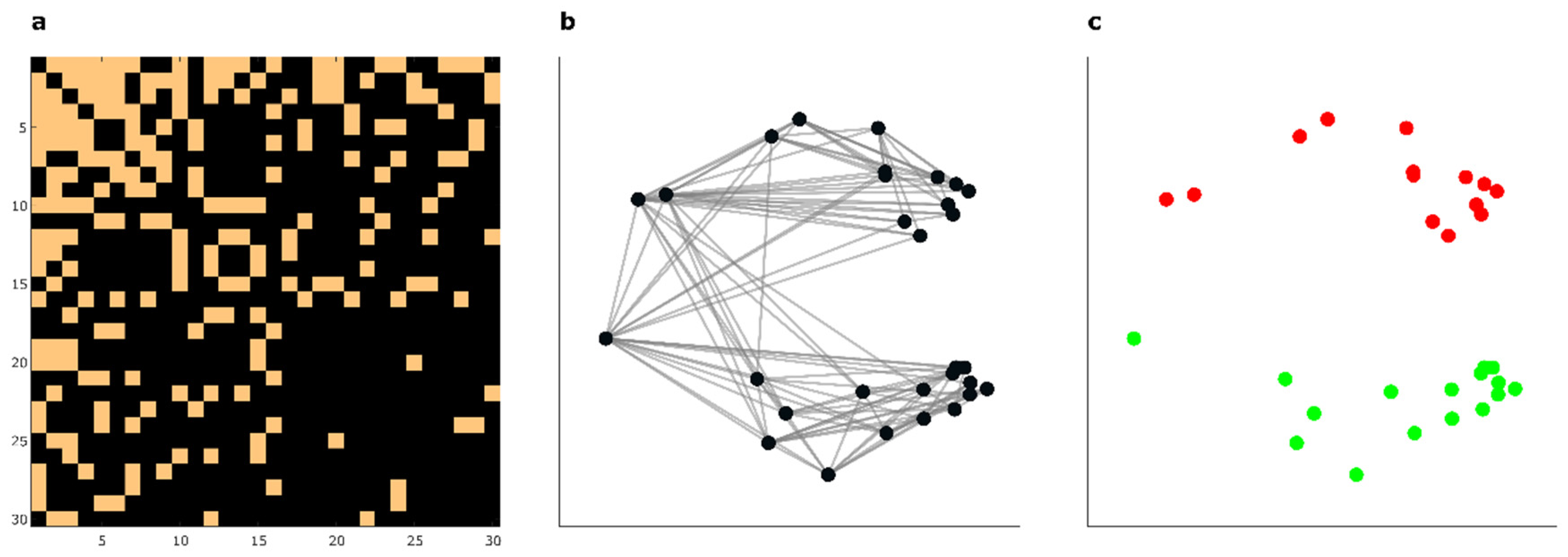
Examples of mesoscale patterns in complex networks are: communities or modules, in-block nestedness, core-periphery structures. In this study we will concentrate on mesoscale patterns associated to community organization because they are investigated in many domains of applied network science. A community or module refers to a subset of nodes within a network that interact with each other more frequently than with nodes outside that specific community [18]. Communities are a crucial meso-property to analyze in order to reveal and understand the emergence of mesoscale mechanisms in the associated complex system, however their visualization is not always straightforward. For instance, Figure 2a displays the adjacency matrix associated with the unweighted network connectivity of an artificial complex network with 2 communities generated with the nPSO model [19,20]. Looking at the Figure 2a binary color visualization (orange color for observed and black color for missing interactions) of the adjacency matrix, it is not straightforward to visually distinguish the presence of mesoscale patterns that can be associated with the 2 communities in the network.

Network embedding in a geometric space of two-dimensions (2D) [21,22] plays a crucial role in the visual representation, discovery, investigation and interpretation of mesoscale patterns hidden in the structure of a complex network. When Figure 2a adjacency matrix is represented by a network embedding algorithm (in this case, HOPE [23]) in a 2D geometric space (Figure 2b), we can visually recognize the presence of the 2 communities (compare their pattern with their ground truth node’s colors in Figure 2c) showing the utility of network embedding to discover patterns in complex data analysis [24,25,26,27]. Yet, new challenges [28] emerge after the data embedding. For instance, how close or far, how similar or distant are these mesoscale structures which are associated to communities in the networks? The calculation of the separability of the communities in the two-dimensional geometric space can be used for instance: (1) to evaluate the performance of network embedding algorithms or to guide the best tuning of their hyperparameters; (2) to evaluate the similarity between the mesoscale organization of diverse complex networks according to the geometric separability of their communities. In the first case, the more the algorithms clearly disclose and display the community structure of the networks in the two-dimensional space, the better their performance is rated. In the second case, the closer is the evaluation of community geometric separability between networks that are generated from the same complex system, the higher is their similarity in their mesoscale organization.

Hence, we introduce and test also in network science the notion of linear and nonlinear geometric separability of mesoscale patterns [1,2] which, in the specific case of this study, concerns measuring the geometric separability of the groups of network’s nodes that form the communities.

Figure 2. Geometric separability of community-based mesoscale patterns in complex networks. (a) The adjacency matrix of an artificial network with two communities generated with the nonuniform popularity similarity model (nPSO). From the adjacency matrix, the presence of any mesoscale structure associated to community organization is not visible (b) Embedding by the HOPE algorithm of the nPSO network in a two-dimensional geometric space reveals the presence of a geometric representation composed by two groups of nodes (one up and one down), providing evidence of network embedding efficacy to visualize the latent mesoscale structure of complex networks. (c) Attributing to each node a color related with the respective community type (red or green) in the network, we note that nodes in the same community locate closer to each other forming two groups in the geometric space. Evaluating the representation of a network in relation to the geometric separability of the groups of nodes formed by their communities is an innovation that we introduce in this article.

Results

Innovations of This Study

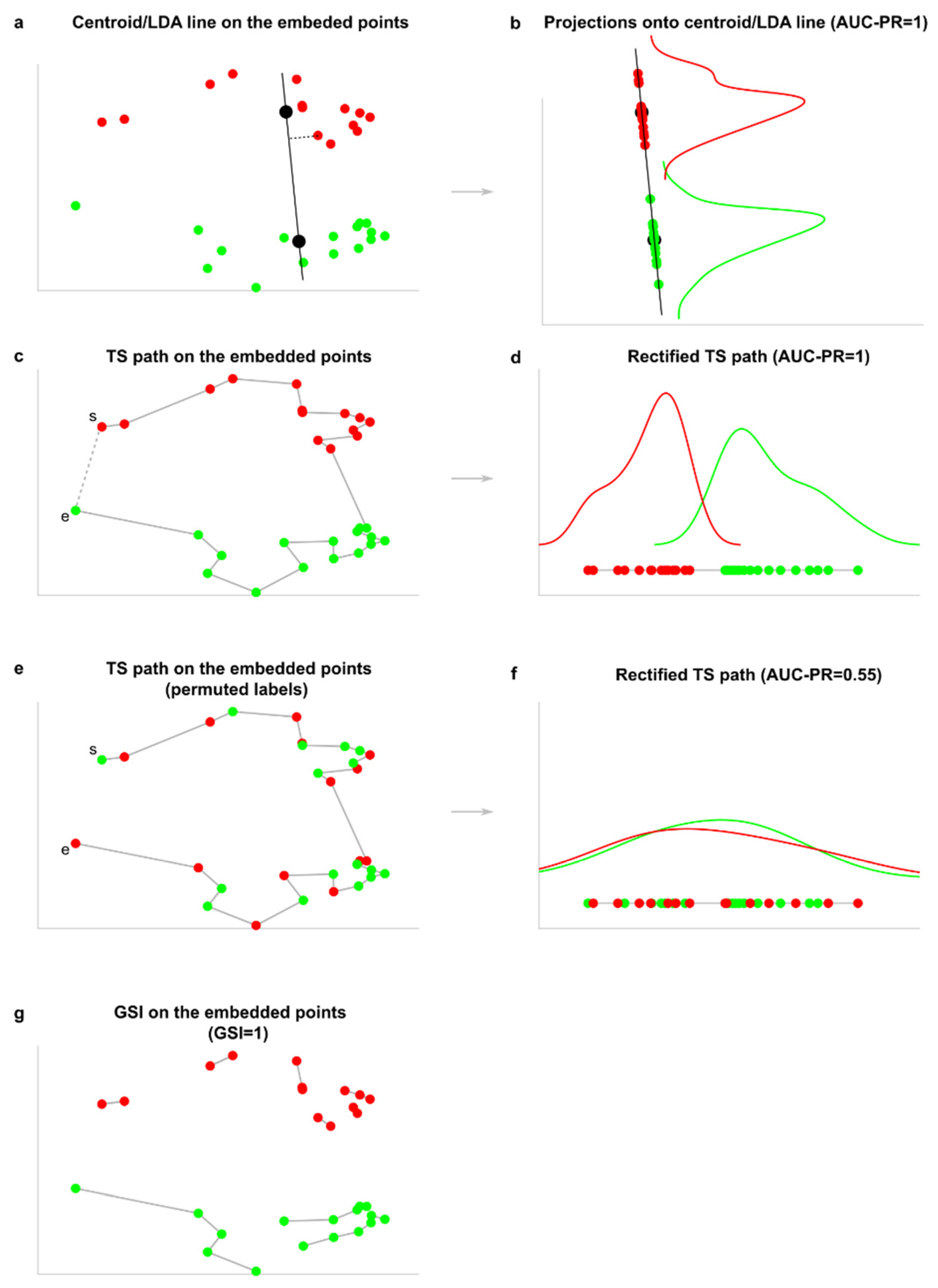
The first innovation of this study is to offer a general definition of projection separability (PS) for points in a geometric space which include also the notion of projection separability curve (PSC) to address nonlinear separability problems. We propose that to assess the geometric separability of two generic sets of points that form mesoscale patterns in a representation space, a measure of projection separability projects or connects the points by ordering them on a line (linear separability, Figure 3a) or a curve (nonlinear separability, Figure 3c) in relation to their geometric proximity in the representation space. The projection separability line/curve represents a 1D projection of the bi-class points that is meaningful (according to a certain discrimination criterion) for their separation in two classes. Once the nodes are projected on a line or curve, a projection separability index (PSI) is defined by applying any bi-class separability measure (such as the area under the curve of precision-recall, AUPR [16], or any other measure for evaluation of unbalanced data classification) directly on the projection line (Figure 3b) or rectified curve (Figure 3d) to measure the extent to which the two groups are separable. For data with a multi-group structure, the average PSI among all pairs of groups is considered as an overall measure. This means that the performance of a PS measure is always between 0 (worst result) and 1 (best result). Note the previous definition of projection separability (PS) provided by Acevedo et al. [2]. was limited to the case of linear separability (Figure 3a,b) evaluated by the projection separability line, which is a sub-case of projection separability curve. In contrast, the geometric separability index proposed by Thornton (GSI) [1] - that is based on the criterion of nearest neighbor label-similarity - offers a solution (Figure 3e) which does not order the points according to their proximity on a curve, hence it cannot be used for projection separability. The example in Figure 3a–d shows that in case of a linear separability problem where the two groups (red and green dots, Figure 3a) are linearly separable in the geometrical space, in principle, both a projection separability line (Figure 3a,b) and a projection separability curve (Figure 3c,d) are able to offer an appropriate quantification of perfect linear separability (AUC-PR = 1, Figure 3b,d). However, in this study we extend our investigation to the case of nonlinear separability problems such as in Figure 5f–i and Figure 6f–n, which we will discuss in the next section Empirical evidence on artificial datasets. At this stage, after having introduced the notion of projection separability curve (PSC), a problem arises on how to estimate it.

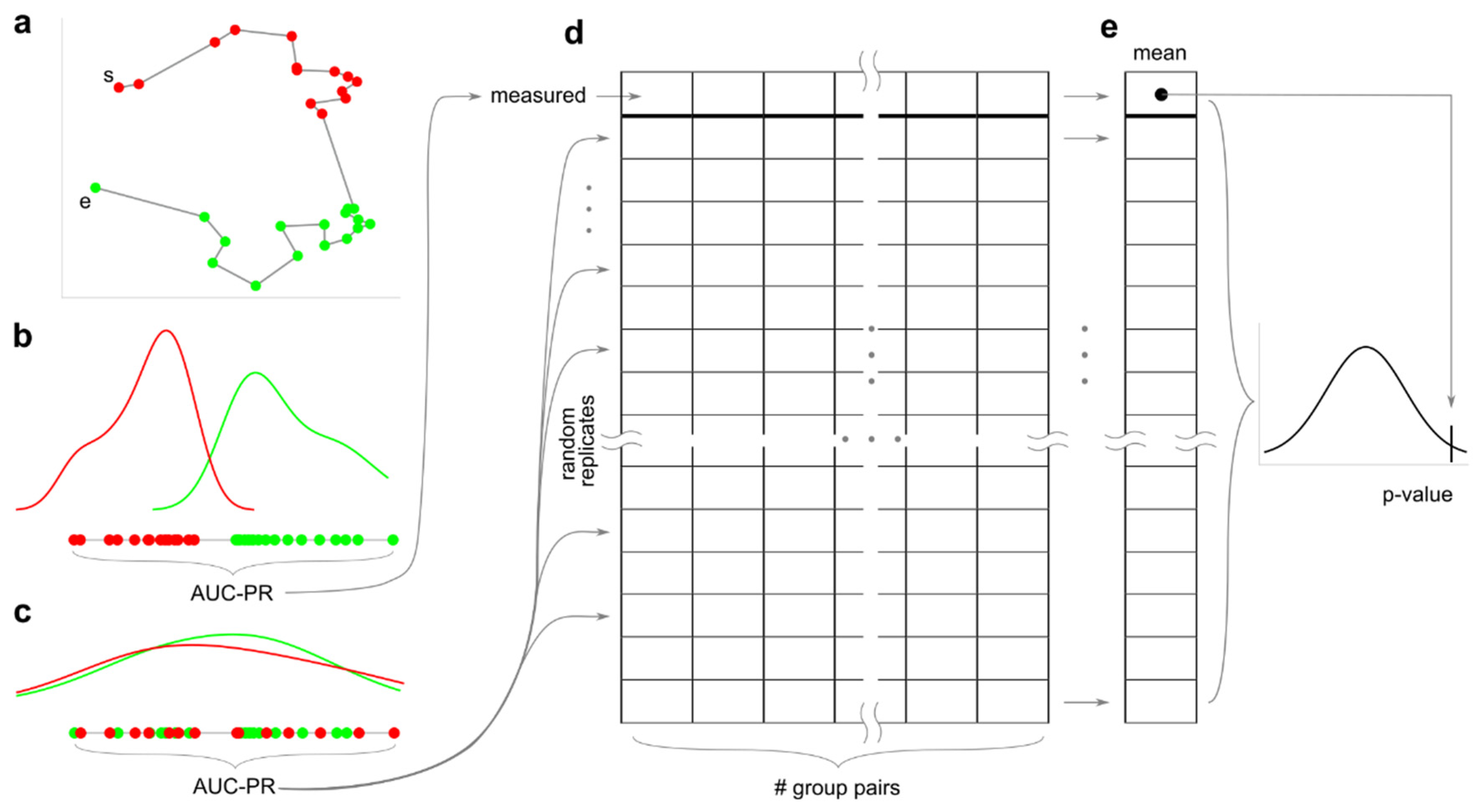
The second innovation is on the methodology to compute a projection separability curve, for which we need to select a criterion of nonlinear separability and optimize it. We propose to approximate the projection separability curve by solving the travelling salesman problem (TSP) via a very efficient TSP solver such as Concorde [29]. The solution of the TSP is a tour (see example in Figure 3c) from which, by removing the connection of maximum length (dashed connection in Figure 3c) between the two groups, we extract the path of minimum length that travels across all the data points or network nodes embedded in a geometric space. We define this type of nonlinear projection separability as travelling salesman projection separability (TSPS) and the associated projection separability curve as travelling salesman projection separability curve (TS-PSC). Therefore, in this study we arrive at a complete and general definition of the projection separability theory according to which we can assess the projection separability of data or network nodes in a geometrical space by using a projection separability line (computed as CPS or LDPS, see previous study of Acevedo et al. [2]) or using a projection separability curve (computed as TSPS) in the case of data spatially organized according to a nonlinear separability problem. As introduced for projection separability line in the previous study of Acevedo et al. [2], also here in the case of projection separability curve we can compute an empirical p-value that expresses the extent to which the PSI measure is statistically significant. Henceforth we visually explain the main steps of the procedure, and the technical details are provided in the Method section. Keeping fixed the solution of the TS-PSC, the ground-truth-group labels (Figure 3c) are shuffled uniformly at random (Figure 3e) and the AUC-PR is computed on the rectified curve (Figure 3f). This process (Figure 4a–c) is repeated several times to create a fixed number m (in this study m = 1000 realizations, see Method section) of random replicates AUC-PR estimations (Figure 4d, m rows of the matrix) for each pair of groups in the data (Figure 4d, columns of the matrix). Then, to build a null model the mean replicate values across the different group pairs (across the columns) is computed and the mean values are used to build a null model distribution (Figure 4e). The empirical p-value is computed considering the proportion (in respect to all the values m + 1: m random values and 1 true measured value) of randomly-generated values that are larger than true-measured (observed) value.

Figure 3. Geometric separability based on projection or first-neighbor strategies. (a) Example of how the centroid projection line (CPS) or the linear discriminant line (LDPS) would be drawn considering the linear geometric separability of the two community-based groups of network nodes in Figure 2c. The two black dots at the center of the plot are the centroids of the respective groups of nodes. (b) The nodes are projected on the projection separability line and the AUC-PR is computed to evaluate the extent of linear separability between the two groups. The AUC-PR can be substituted by any other bi-class classification measure for unbalanced data. (c) Travelling salesman tour (with the dashed line) and path (without the dashed line) across the points that are the nodes of the nPSO network (Figure 2) embedded in the two-dimensional space (Figure 2c). The travelling salesman (TS) path approximates the projection separability curve that accounts for the intrinsic nonlinear geometry of the data points. (d) The nodes are aligned on the rectified TS path and the AUC-PR is computed to evaluate the extent of separability between the two groups. (e) and (f) are respectively equivalent to (c) and (d) when the labels of the two communities are uniformly at random reshuffled to generate one instance of the null model. (g) The geometric separability index adopts a strategy defined as the proportion of data points whose classification labels are the same as those of their first-nearest neighbor.

The third innovation is to introduce in network science the concept of projection separability of the community’s nodes of a complex network represented in a geometric space (community projection separability, CoPS). For a network whose nodes lie or are embedded in a geometric space, in order to assess the geometric separability of nodes across two communities, we can project or connect their nodes on a projection separability line or curve. According to this definition of coPS we can compute any projection separability index (PSI), which is calculated by applying any bi-class separability measure (such AUC-PR [16]) directly on the projection line (Figure 3b) or rectified curve (Figure 3d) to measure the extent to which the two groups are separable. For networks with a multi-community structure, the average PSI among all pairs of communities is considered as an overall measure. This means that the performance of a PS measure is always between 0 (worst result) and 1 (best result). Note that there exist many criteria to define the separability of community directly from the network structure, such as modularity [30], and they are used to implement community detection algorithms. However, here our innovation is to propose a criterion to evaluate the representation of a network in a geometric space with respect to the quality of representation of its mesoscale community structure. And, for representing at the best the mesoscale community structure in a two-dimensional space, we intend that the nodes should preserve in the geometric space both inter-community diversity and intra-community diversity. In addition, for each PSI evaluation on the community projection separability, an empirical p-value that expresses the statistical significance of PSI evaluation is computed according to the procedure described above in this section.

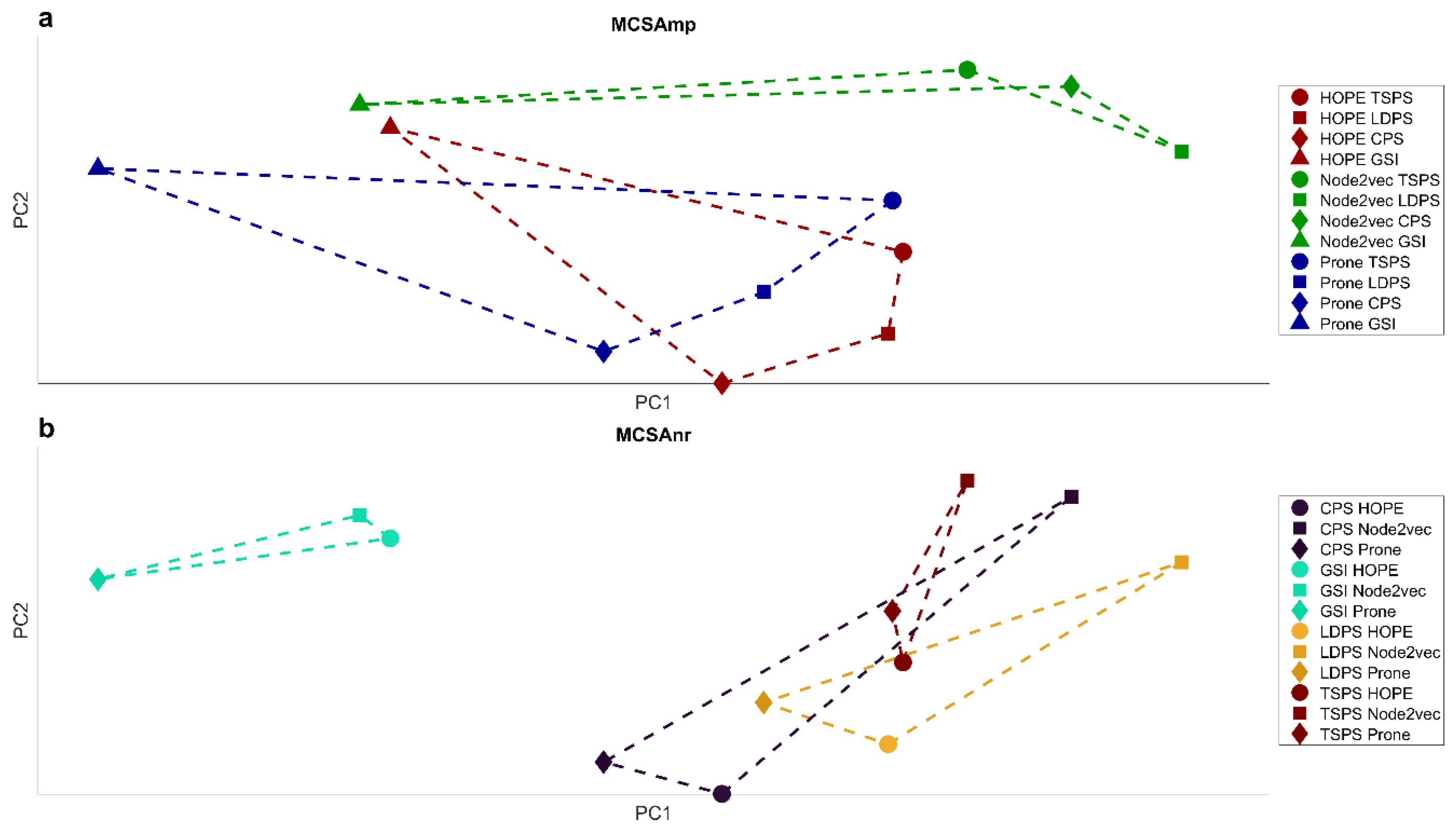
The fourth innovation of this study is in multidimensional analysis of the network community organization. We propose a multivariate analysis that we name multivariate community separability analysis (MCSA), which adopts principal component analysis (PCA) to represent in a 2D space two different scenarios: (i) the first scenario, that we call multivariate community separability analysis of the methods’ performances (MCSAmp), considers how similar are the performances of the embedding methods evaluated using different community projection separability measures in respect to features which are the values of community projection separability across different networks; (ii) the second scenario, that we call multivariate community separability analysis of the network representations (MCSAnr), considers how similar are the network representations obtained using different embeddings in respect to features which are the values of community projection separability across different measures. In the section below Empirical evidence on real network, we will discuss the applications of MCSA on real data from network science.

Empirical Evidence on Artificial Datasets and the Adaptive Geometrical Separability (AGS)

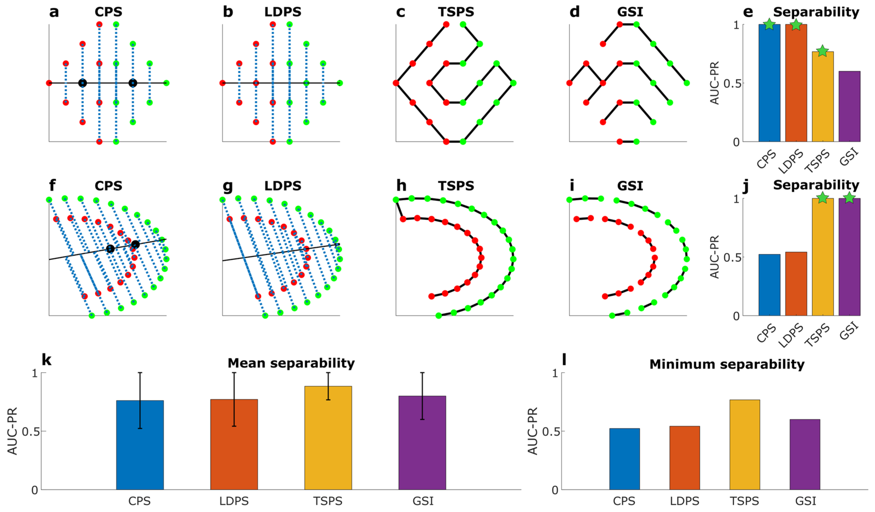
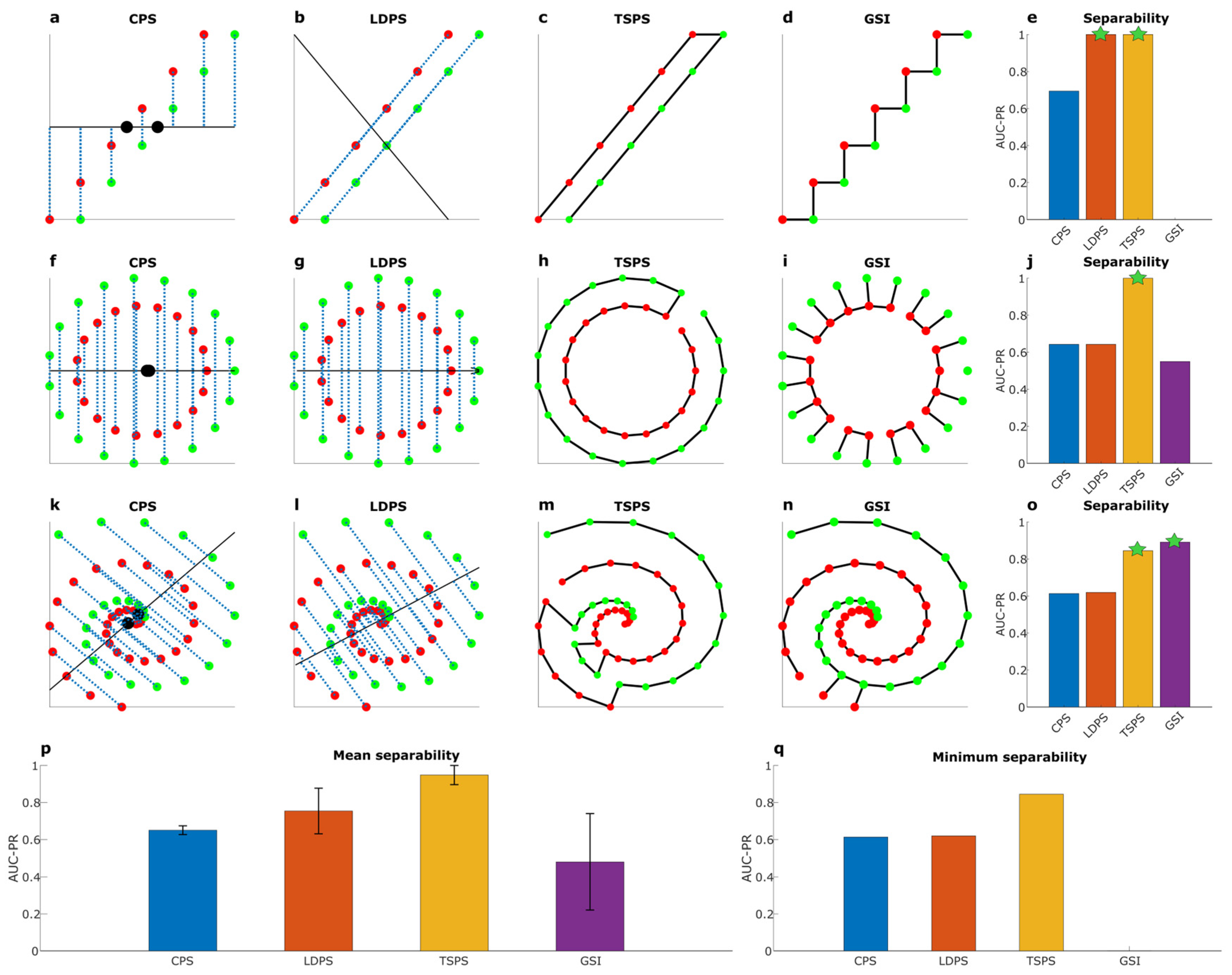
Figure 5 showcases performance of geometric separability measures when they are tested on artificial datasets with linear and nonlinear separability problems in complex data science. Figure 5e shows that CPS and LDPS perform better than TSPS and GSI in the provided linear separability problem (Figure 5a–d), offering evidence that, when a problem is linearly separable, their performance (estimated using the area under the precision-recall curve, AUPR) might overcome the one of nonlinear methods. Note that the geometric separability estimated by GSI is the only not statistically significant (Figure 5e, green stars indicate statistical significance with p-value < 0.01). Conversely, Figure 5j shows that CPS and LDPS perform worse than TSPS and GSI in the provided nonlinear separability problem (Figure 5a–d), offering evidence that, when a problem is nonlinearly separable, the nonlinear methods can overcome the linear ones. Note that the geometric separability estimated by CPS and LDPS are not statistically significant (Figure 5j, green stars indicate statistical significance with p-value < 0.01). When we take the mean performance (Figure 5k) of these methods across the two problems, TSPS performs the best, meaning that TSPS is the most versatile method. Besides, when we take the minimum performance (Figure 5l) across the two problems, TSPS performs again the best meaning that it is the most robust method. The stars in Figure 5e,j indicate that TSPS is the only measure statistically significant in both cases, indicating that TSPS produces estimations which can be reliable regardless of the linear or nonlinear origin of the problem.

Figure 5. Linear and nonlinear separability in complex data science. Red and green dots indicate the samples of two different groups. (a-e) refer to an example of a linearly separable dataset called Rhombus. (f-j) refer to an example of a nonlinearly separable dataset called Halfkernel. (a, f) centroid projection separability (CPS): the two black dots indicate the centroids (median estimator) of the two groups of samples, the black line indicates the projection line, the vertical blue dashed lines indicate the projections of the samples. (b, g) linear discriminant projection separability (LDPS): the black line indicates the first component projection vector of the linear discriminant analysis (LDA), the other graphics are as for (a). (c, h) Travelling salesman projection separability (TSPS): the travelling salesman path across the samples is indicated by the black solid lines. (d, i) geometrical separability index (GSI): the black solid lines indicate the first neighbor sample matching. (e, j) separability of each measure in the respective dataset: (e) Rhomboid and (j) Halfkernel. (k, l) mean and minimum separability of each measure across the two datasets. In (e, j) the values of the indices with a significant (p-value < 0.01) geometric separability are marked with a star, which means that these values are very unlikely to be obtained by chance.

Figure 6 displays the performance of the same methods on three different examples of hard separability problems, where the term ‘hard’ in this context means difficulty to detect the presence of separability. The first example (Figure 6a–d) presents the difficulty of two groups that are linearly separable but are very close to each other. Figure 6e provides a bar plot that compares the results of the different separability measures. In this scenario: CSP (Figure 6a) suffers from bad performance because it detects a wrong linear separability line; GSI (Figure 6d) suffers from null performance because it matches pairs of samples of the opposite classes; LDPS (Figure 6b) and TSPS (Figure 6c) offer the perfect solution. LDPS and TSPS only are statistically significant (Figure 6e, green stars indicate statistical significance with p-value < 0.01). The second example (Figure 6f–i) present the difficulty of two groups that are nonlinearly separable because they are concentric circles with different radius. Figure 6j provides a bar plot that compares the results of the different methods. In this scenario: CSP and LDPS (Figure 6f,g) suffer from the same bad performance because they detect the same linear separability line that does not assess the correct separability, indeed this is a nonlinear problem, hence it is by definition linearly unsolvable; GSI (Figure 6i) also suffers from bad performance because it occasionally matches pairs of samples of the opposite class; TSPS (Figure 6h) offers the perfect solution which is also statistically significant (Figure 6j, green stars indicate statistical significance with p-value < 0.01). The third example (Figure 6k–n) presents the difficulty of two groups that are nonlinearly separable because they are following two concentric spirals of different radius. Figure 6o provides a bar plot that compares the results of the different methods. In this scenario: CSP and LDPS (Figure 6k,l) suffer from bad performances because they detect two different linear separability lines that do not assess the correct separability, indeed this is a nonlinear problem, hence it is by definition linearly unsolvable; GSI (Figure 6n) offers the best but still not the perfect solution; TSPS (Figure 6m) offers the second best result because the solution to the TSP provided by Concorde algorithm suffers of few jumps that result in wrong connections across the two different groups. TSPS and GSI only are statistically significant (Figure 6o, green stars indicate statistical significance with p-value < 0.01). When we take the mean performance (Figure 6p) of these methods across the three problems, TSPS performs the best, meaning that TSPS is the most versatile method. Besides, when we take the minimum performance (Figure 6q) across the three problems, TSPS performs again the best, meaning that is the most robust method. The stars in Figure 5e,j,o indicate that TSPS is the only measure statistically significant in the three cases, indicating that TSPS produces estimations which can be reliable regardless of the ‘hardness’ of the problem.

Results on these artificial datasets show that TSPS is the most versatile and robust of the four tested measures for separability estimation; however, different measures can magnify their performance in relation to the different types of separability problems. Therefore, we propose an adaptive geometrical separability (AGS) estimation that, for each type of dataset (or network), can assess the extent to which the groups in the data (or communities in networks) present linear or nonlinear empirical separability, and can identify the best solver (i.e., measure) to achieve such maximal separability performance.

Figure 6. Hard separability problems in complex data science. Examples of hard separability problems, the term ‘hard’ indicates difficulty to detect the presence of separability. (a-e) refer to an example of a linearly separable dataset called Parallel lines. (f-j) refer to an example of a nonlinearly separable dataset called Circles. (k-o) refer to an example of a nonlinearly separable dataset called Spirals. (a, f, k) Centroid projection separability (CPS): the two black dots indicate the centroids (median estimator) of the two groups of samples, the black line indicates the projection line, the vertical blue dashed lines indicate the projections of the samples. (b, g, l) Linear discriminant projection separability (LDPS): the black line indicates the first component projection vector of the linear discriminant analysis (LDA), the other graphics are as for (a). (c, h, m) Travelling salesman projection separability (TSPS): the travelling salesman path across the samples is indicated by the black solid lines. (d, i, n) Geometrical separability index (GSI): the black solid lines indicate the first neighbor sample matching. (e, j, o) separability of each measure in the respective dataset: (e) Parallel lines, (j) Circles and (o) Spirals. (p, q) mean and minimum separability of each measure across the three datasets. In (e, j, o) the values of the indices with a significant (p-value < 0.01) geometric separability are marked with a star, which means that these values are very unlikely to be obtained by chance.

Empirical Evidence on Real Complex Multidimensional Data

Figure 7 reports results on the radar signal dataset [31], which is a benchmark for testing the ability of embedding techniques to solve the crowding problem [32], which means that after two-dimensional embedding, the different groups of samples tend to collapse on top of each other (highly overlapping) in the representation space. Hence, evaluating the correct group separability is challenging and the complexity of this dataset is associated with the mix of hierarchical and similarity relations between the data samples (radar signals) in a multidimensional feature space. Indeed, the radar signal dataset is composed good radar signals that are highly similar, and bad radar signals that are highly dissimilar. It counts 350 valid samples, 34 features, and three groups: good radar signal, bad radar signal type1 and bad radar signal type2. We performed the embedding in the two-dimensional space considering two baseline methods, and we specifically selected them since they are based on different and complementary principles of embedding. Minimum Curvilinear Embedding (MCE) [21] is an approach for data embedding that leverages the hierarchic topological information of the data and it is parameter-free, hence offering a unique solution. t-Distributed Stochastic Neighbor Embedding (t-SNE) [33] minimizes the Kullback-Leibler divergence between the joint probabilities of the low-dimensional embedding and the high-dimensional data, it presents the hyperparameter perplexity (p), which is a smooth measure of the effective number of neighbors and accounts for the balance between local and global aspects of the data. In our tests the perplexity p of t-SNE was fixed to the value that offered the best average performance across the tested geometric separability measures.

MCE is able to address quite well the crowding problem which displays an intrinsic hierarchical mesoscale structure of the radar signal dataset (Figure 7a), therefore all the four tested geometric separability measures perform similarly well (Figure 7b), offering statistically significant results (Figure 7b). t-SNE is based on an embedding strategy that suffers more for data with highly intrinsic hierarchical mesoscale structure, indeed the representation in the two-dimensional space is more crowded (Figure 7c). This results in the performance of the geometric separability measures being all statistically significant but not homogenous: LDPS and GSI indicate higher separability than CPS and TSPS. However, according to the adaptive geometrical separability (AGS) strategy we should select as final estimation the highest, which is provided by GSI. GSI’s value on this t-SNE representation is in the same range but lower than the values of geometric separability on the MCE representation, indicating that MCE works better than t-SNE for representing the intrinsic mesoscale structure of the multidimensional data. This example helps to understand how to evaluate the quality of embedding and visual representation of real complex multidimensional data considering the geometric separability measure of their mesoscale group structure.

Empirical Evidence on Real Complex Networks

In this section, we report the results of applying our methodology to eight real social networks with different community organizations. The Zachary’s Karate Club represents the friendship between the members of a university karate club in the United States (US). Its two communities are formed by splitting the club into two parts, each following one different trainer. The four Opsahl networks are intra-organizational networks: Opsahl_8 (7 communities), Opsahl_9 (7 communities), Opsahl_10 (4 communities), and Opsahl_11 (4 communities). The Polbooks network represents frequent co-purchases of books concerning US politics on amazon.com. Its three communities are associated with the political orientation of the books as either conservative, neutral or liberal. The Football network presents games between colleges during the regular season in the fall of 2000. Its 12 communities are the conferences that each team belongs to. The Polblogs network consists of links between blogs about the politics in the 2004 US presidential election. Its two communities represent the political opinions of the blogs (right/conservative and left/liberal). More details about these network datasets are provided in the methods section.

Furthermore, we investigate the performance of three baseline methods for network embedding: HOPE [23] has one hyperparameter to tune that we set to the default value, because according to some preliminary tests we found it does not substantially change the embedding in a way that is relevant for this study; ProNE [34], which does not have hyperparameters to tune and also provides a sparse matrix factorization version called ProNE (SMF); and Node2vec [35], which has two hyperparameters to tune (return parameter

p

and inOut parameter

q

) that we fine-tuned to select the best performance, because according to some preliminary tests we noted they substantially change the embedding in a way that is relevant for this study. The rationale behind selecting these three embedding methods lies in their diverse computational strategies, which provide a wide spectrum of potential results for testing in our study. HOPE (High-Order Proximity Preserving Embedding) is a matrix-factorization-based technique that preserves high-order proximities within networks. It captures the symmetric transitivity present in large-scale graphs. ProNE (Proximity Network Embedding) is a sparse matrix factorization method specifically designed to address scalability challenges in complex and large networks, retaining localized and global clustering network information. Node2vec is a skip-gram-based approach that focuses on generating feature representations that maximize the likelihood of preserving network neighborhoods in a reduced-dimensional space. It achieves this by employing a second-order random walk strategy. More details about these embedding algorithms are provided in the methods section.

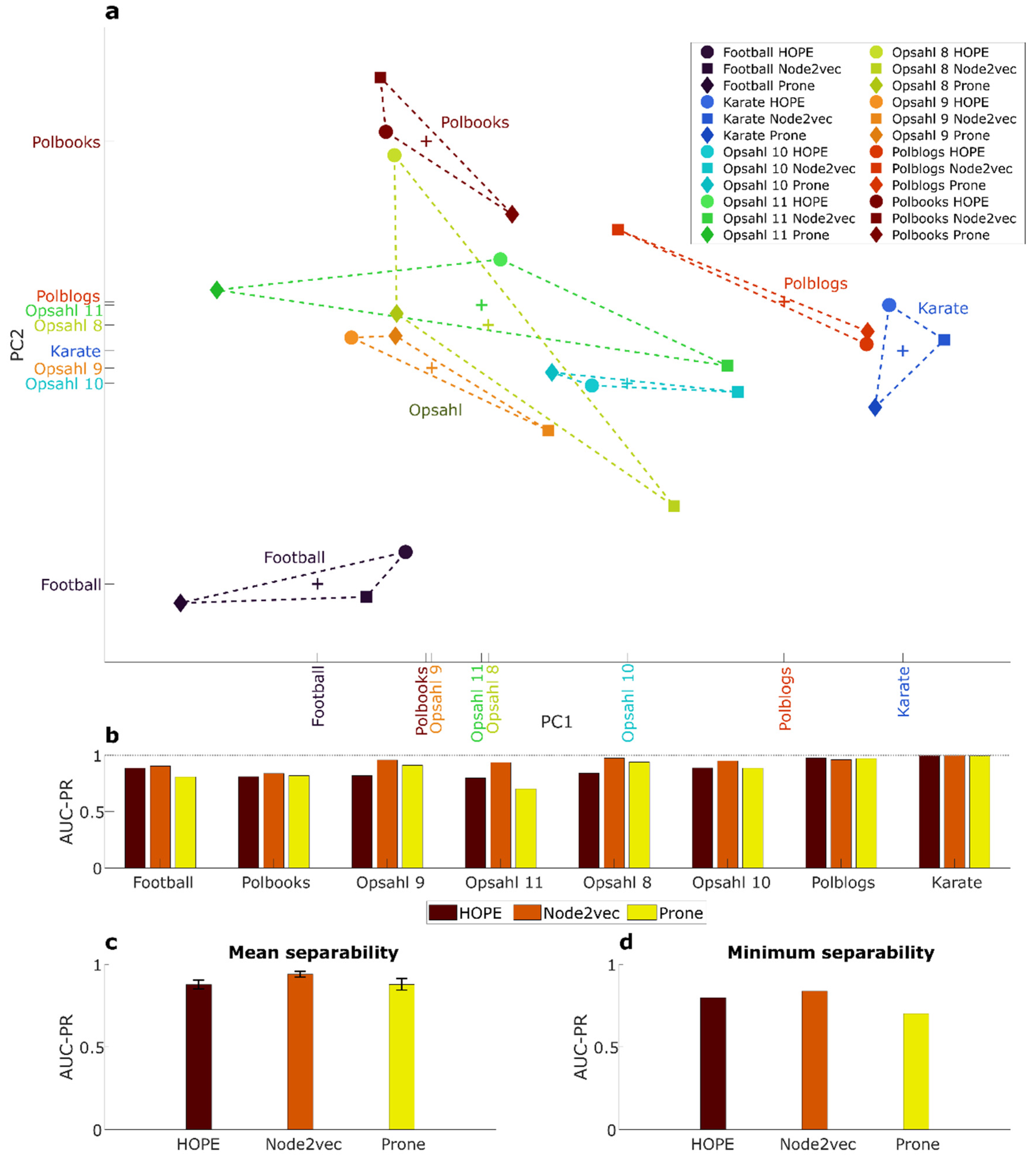
Figure 8a,b display the same representation edited according to different graphic settings, and they report the result of the multivariate community separability analysis of the methods’ performances (MCSAmp). Each data point indicates the performance of an embedding method according to a certain community separability measure evaluated in the multidimensional space of the eight networks and embedded by PCA in a two-dimensional space of principal components one and two (PC1 and PC2, respectively). Figure 8a is created by connecting the data points that indicate the same type of embedding method: the polygon (green) formed by Node2vec performances is far from the ones of ProNE and HOPE that are overlapping. This result indicates that ProNE and HOPE have a similar embedding performance that differs from Node2vec. Figure 8b is created by connecting the data points that indicate the same type of community separability measure: the triangle (green) formed by GSI evaluations is far from the overlapping ones of CPS, LDPS, and TSPS. This result indicates that CPS, LDPS and TSPS have a similar evaluation trend that differs from GSI, which can be explained by their common projection separability nature. The triangle (brown) formed by TSPS is smaller than the triangles formed by the other projection separability measures; this means that TSP produces evaluations that are closer to each other and, therefore, more consistent across different embedding methods than the other projection separability measures.

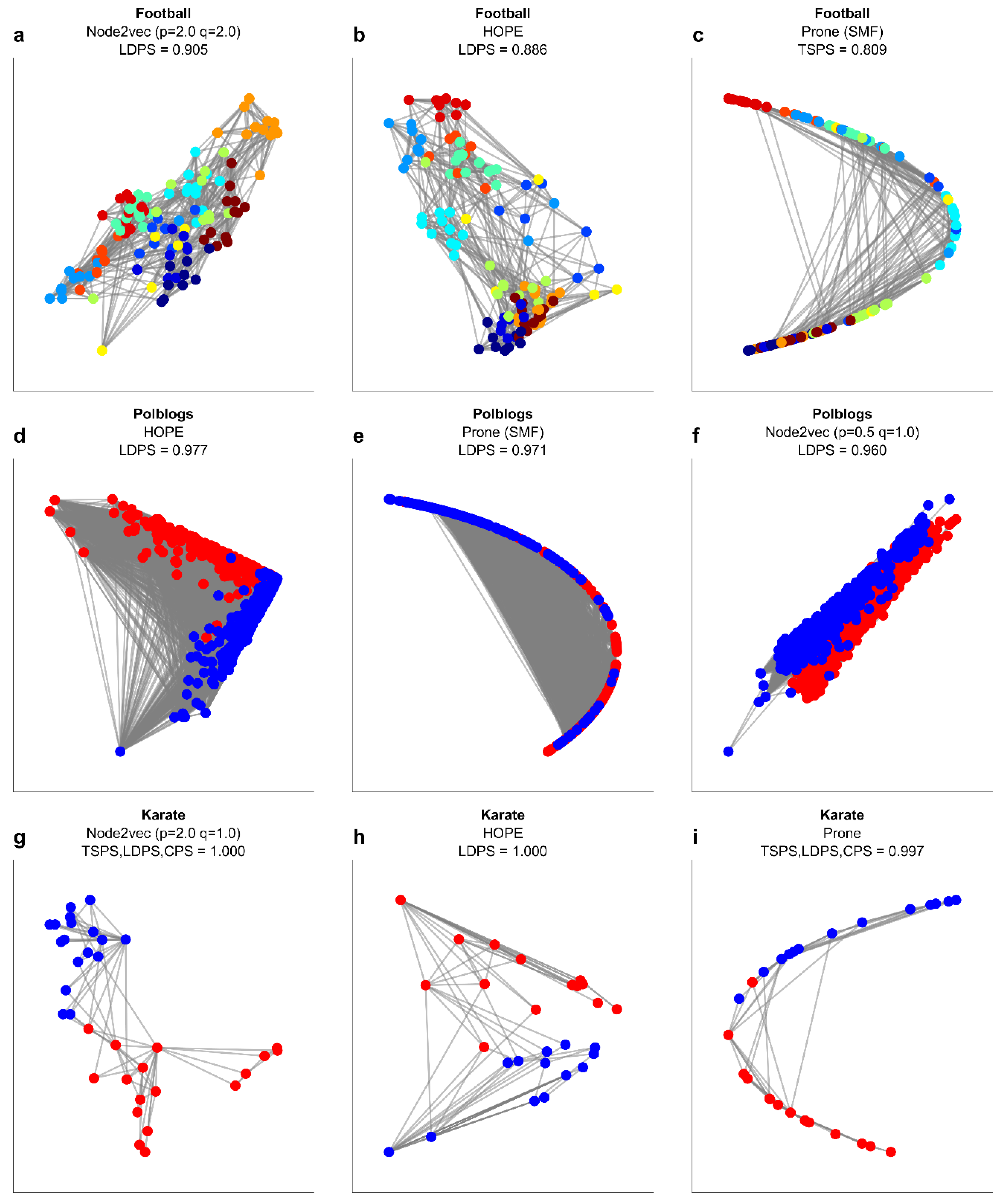
Figure 9a reports the result of the multivariate community separability analysis of the network representations (MCSAnr). Each data point indicates the community separability of a specific network according to an embedding method evaluated in the multidimensional space of the 4 community separability measures and embedded by PCA in a two-dimensional space of principal components one and two (PC1 and PC2, respectively). The data points that indicate the same type of network are connected. The two triangles formed by Football and Karate are at opposite sides of the PC1 axis, indicating that these networks largely differ in the level of community separability. Indeed, Figure 9b reports the adaptive geometric separability (AGS) level for each embedding method in each network, and precisely, Football’s AGS levels are lower than the Karate ones. This is visually evident in Figure 10, where the 2D embeddings of Football according to Node2vec (Figure 10a), HOPE (Figure 10b) and ProNE (Figure 10c) display a lower separability of the 12 communities with respect to the 2D embeddings of Karate, for which the separability of the 2 communities is perfect (value 1) in case of Node2vec (Figure 10g) and HOPE (Figure 10h), and almost perfect (value 0.997) for ProNE. Besides, all these results reported a significant geometric separability (p-value < 0.01). The two triangles formed respectively by Karate and Polblogs are on the same side (right) of the PC1 axis, indicating that these networks should have a comparable level of community separability, although for Polblogs it should be slightly lower because Karate has the highest PC1 coordinate. Indeed, in Figure 9b, Karate’s AGS levels are comparable with Polblogs ones but slightly higher. This is visually confirmed in Figure 10, where the 2D embeddings of Polblogs according to Node2Vec (Figure 10d), HOPE (Figure 10e) and ProNE (Figure 10f) display a lower separability of the 2 communities with respect to the 2D embeddings of Karate (Figure 10g–i), for which the separability of the 2 communities is perfect or almost perfect. The four triangles of the respective 4 Opsahl networks are partially overlapping at the center of the figure, indicating that they have comparable levels of community separability, which is confirmed in Figure 9b observing at their AGS levels. From Figure 9c, which reports the minimum and mean AGS of each embedding method across the networks, Node2vec emerges as the most versatile and robust method, offering the 2D representation with the highest community separability across the investigated methods. However, Node2vec has two hyperparameters to fine-tune; therefore, it makes sense that it has larger versatility and wider margin to improve performance than HOPE and ProNE.

Discussion

We provide a framework for the definition and measure of the linear and nonlinear geometric separability of mesoscale patterns in 2D visualization of complex data and networks. We adopt two linear measures and two nonlinear measures. One of these nonlinear measures is proposed in this study, and it is based on solving the travelling salesman problem (TSP). Then, we focus on applications, investigating both real complex multidimensional data and real networks visual representations in a two-dimensional space. We measure the extent to which the embedding of data or networks in a two-dimensional space can produce a representation that unfolds its mesoscale structure, which means to represent distinguishable group in multidimensional data or communities in networks. Yet, without loss of generality, the tools we propose can be applied to measure group separability in a geometrical space of any dimensionality.

In our previous study [2] we introduced a methodology to measure linear separability based on a projection separability line, in this study we extend this methodology to measure also nonlinear geometric separability introducing as innovation the projection separability curve. We propose to approximate the projection separability curve by solving the travelling salesman problem (TSP) via a very efficient TSP solver such as Concorde [29] algorithm. The solution of the TSP is a tour from which is obtained the path of minimum length that separates the groups/communities travelling across all the data points or network nodes embedded in a geometric space. We define this type of nonlinear projection separability as travelling salesman projection separability (TSPS). We stress this is the first time in literature that the TSP is employed to define a criterion of nonlinear separability of data in a geometric space, hence the idea to redefine a problem of nonlinear geometric separability as a specific case of the travelling salesman problem is an innovation both in computer science and complex data analysis.

Results on artificial and real multidimensional datasets show in which scenarios TSPS is the only method offering a fair assessment of nonlinear geometrical data separability. In contrast, we comment on other cases in which mere linear projection separability is more appropriate. Therefore, we propose an adaptive geometric separability (AGS) method that, for each type of dataset (or network), can assess the extent to which the group (or community) separability is linear or nonlinear, and what is the best solver to achieve such geometrical group separation.

The motivation to investigate real applications in network embedding is that this field has been developing as a vibrant research topic in recent years [23,24,34,35], and the study of appropriate ways to evaluate its performance is currently on the verge [36]. The most employed strategies are task-oriented evaluations applied to the network or its node embedded in the geometric space, for instance: link prediction [37], geometric-weighted network community detection [24], node clustering, etc. [38,39]. These approaches rely on applying unsupervised algorithms whose performance in a specific task is considered a reference to assess the quality of the network embedding. Differently from these past methodologies, in this study we diverge from a task-oriented evaluation of embedding, and we propose to evaluate the ability of an algorithm to preserve the mesoscale organization of a network, which means to offer a 2D representation that discloses and clearly depicts the community organization. Hence, one of our innovations is to introduce in network science the adoption of a criterion that distinguishes between linear and nonlinear separability of communities in a geometric space to evaluate the network representation.

The final innovation of this study is to propose a multivariate analysis that we name multivariate community separability analysis (MCSA), which adopts principal component analysis (PCA) to represent in a 2D space two different scenarios: (i) how similar are the performances of embedding methods evaluated using different community projection separability measures in respect to the values of community projection separability across different networks; (ii) how similar are the network representations obtained using different embeddings in respect to the values of community projection separability across different measures. We test and validate these multivariate community separability analyses on real networks, discovering similarities between embedding methods, analogies between separability measures, and affinities between networks’ mesoscale structures.

Altogether, these innovations pave the way toward defining quantitative tools for analyzing the linear and nonlinear separability of mesoscale patterns in complexity science and pattern recognition.

Some limitations to consider for investigation in future studies are discussed hereafter. Although Concorde [29] algorithm is a very efficient TSP solver, the computation of large datasets with hundred thousand of points can be time consuming. Hence the definition of new efficient criteria to approximate the projection separability curve should be considered as an interesting direction of research. For instance, solutions provided by greedy algorithms such as the minimum spanning three cold be compared with the TSP. This study is focused on evaluation of geometric group separability in a two-dimensional visual representation space, however the same methods (without necessity of any formal adjustment) could be used in the future to investigate geometric separability in higher dimensional space.

The possible implications and applications of our research on geometric separability of network community in various fields, such as biological networks, transportation systems, and more is straightforward. For instance, we could apply the multivariate community separability analysis (MCSA), to evaluate how different are the brain MRI structural connectome representations of control and unhealthy subjects considering the mesoscale lobular brain organization, which has been proven to be reflected in the brain connectome topology and geometry [40,41]. Or to evaluate the geometric separability of gene communities in co-expression networks across different tissues [42]. Similarly, we could compare the difference in modular organization of the transportation network of different cities and relate their similarity or diversity in geometric separability of their modules to possible difference in transportation efficiency [43]. Through this study we applied a simplification that is to consider the community structure as a main example of mesoscale pattern in complex networks. This can be view as a limitation. For instance, other mesoscale structures such as echo chambers in social [44] and political [45] networks are an interesting phenomenon which could be investigated by applying geometric separability analysis. Investigating these research topics in future studies would not only demonstrate the versatility and adaptability of the proposed geometric separability analysis, but also its potential impact and utility in different real-world contexts. We hope that this discussion could motivate other scientists to bring forward research on geometric separability of mesoscale patterns in network science. This could significantly enhance the robustness of the findings presented in this study and underscore the broad applicability of the geometric separability measures to data emerging from various complex systems.

Methods

Data and Algorithms

Synthetic Data Generation

In Figure 1, we generated an artificial network with 2 communities by using the nonuniform popularity similarity (nPSO) model [19,20] (available at https://github.com/biomedical-cybernetics/nPSO_model) with the following parameters’ values: 30 as the total number of nodes, 4 as the half of average node degree, a temperature value of 0.1, a gamma value equal to 3, and 2 as the number of communities.

In Figure 2 and Figure 3, we generated five small synthetic datasets with different shapes as a proof of concept to visualize and to inspect the differences between the linear and nonlinear separability measures described below. All datasets are composed of two main groups in a two-dimensional geometrical space.

Rhombus: It contains 20 samples (i.e., data points) arranged in a rhombus-like shape, with each group distributed on each side of the rhombus (i.e., each group is composed of 10 data points). Both groups have close proximity in the center of the shape.

Halfkernel: It contains 35 samples, but in this case, they are arranged in a halfkernel shape. The groups are separated by the two concentric semicircles, where the inner semicircle contains 15 data points, and the outer circle contains 20 data points.

Parallel lines: It contains 12 samples arranged as two parallel lines, each representing one of the two groups (i.e., each group is composed of 6 data points). The distance between the two lines is minimal; thus, the data points of the two different groups are very close to each other.

Circles: It is composed of 40 samples distributed as two concentric circles of different radius, each representing one of the two groups (i.e., each group is composed of 20 data points). The distance between the two circles is minimal; thus, the data points of the two different groups are very close to each other.

Spirals: It contains 55 samples distributed as two concentric spirals, each representing the two groups. The inner spiral contains 32 data points, whereas the outer spiral contains 23 data points. Both spirals have a common origin and separate as they get bigger.

These datasets are provided in the GitHub repository reported in the data availability section below.

Real Complex Multidimensional Data

The radar signal dataset [31] was recovered from the UC Irvine Machine Learning Repository (available at http://archive.ics.uci.edu/ml/datasets/Ionosphere). It contains 350 valid radar signals targeting free electrons in the ionosphere. Shieh et al. [32] studied this dataset using two labeled groups (good and bad radar signals). However, they highlighted that good radar signals are highly similar and bad radar signals dissimilar. Later, Cannistraci et al. [21] confirmed that the bad radar signals can be interpreted as two diverse subcategories (two different groups) that are difficult to identify because of their high nonlinearity (elongated and irregular high-dimensional structure). Hence, in this study we consider the presence of three groups: good radar signal, bad radar signal type1 and bad radar signal type2.

Real Complex Networks

In this study, we considered eight real networks representing different social systems with mesoscale community structural organization. The networks have been transformed into undirected, unweighted, without self-loops, and only the largest connected component has been considered as in [20]. In addition, information about their ground truth communities is available.

The Zachary’s Karate Club [46] (referred to as “Karate”), which contains 34 nodes and 78 edges. It represents the friendship between the members of a university karate club in the United States (US). It has two communities, formed by splitting the club into two parts, each representing a group of members following one trainer.

The American football network (referred to as “Football”), which contains 115 nodes and 613 edges, and represents the matches between Division IA of colleges in the fall of 2000 [18]. It is composed of twelve communities, which are the conferences each team belongs to.

The following networks (Opsahl 8, 9, 10, and 11) were downloaded from https://toreopsahl.com/datasets/. They represent an intra-organizational network described in [47]. Particularly, the networks Opsahl 8 and Opsahl 9 are the representation of a consulting company where the nodes represent employees. Opsahl 8 contains seven communities and has 43 nodes and 193 edges, indicating a link between employees who have at least turned to a co-worker for work-related information seldom. Similarly, Opsahl 9 contains seven communities, 44 nodes, and 348 edges; however, in this case, the links represent a relation between employees who consider the expertise of a co-worker important in the kind of work they do. On the other hand, Opsahl 10 and Opsahl 11 are networks that describe the interactions of a manufacturing company where the nodes represent employees. Opsahl 10 contains four communities, 77 nodes, and 518 edges, where the communities indicate the company locations (Paris, Frankfurt, Warsaw, and Geneva) where the employees were linked by which of their co-workers provided them - frequently or very frequently - with the information they used to accomplish their work. Similarly, Opsahl 11 contains the same number of communities and nodes but 1088 edges, where the employees were linked by their awareness of each other’s knowledge.

Polblogs [48], which contains 1222 nodes and 16714 edges describing the links between blogs about politics in the 2004 US presidential election. It has two communities that represent the political tendencies of the blogs, such as conservative or liberal.

Polbooks (available at http://www-personal.umich.edu/~mejn/netdata/), which contains 105 nodes and 441 edges representing frequent co-purchases of books concerning US politics on amazon.com. It has three communities, each representing a political orientation, such as conservative, neutral, and liberal.

Network Embedding Methods

If we denote an undirected network as

G (V = \{1, \dots, n\}, E)

, i.e., as an abstract structure that is used to model a set

E

of relations (edges) over a set

V

of entities (nodes). Then, the main goal of network embedding is to find a mapping function

f : V \mapsto R^{d}

that projects each node into a d-dimensional space (where

d ≪ |V|)

by preserving as much as possible the structural properties of the network (e.g., similar nodes in the network are embedded close together) [34,49,50]. With the aim of assessing if a network embedding provides a correct low-dimensional representation of a network, we used three state-of-the-art network embedding techniques, such as HOPE [23], ProNE [34], and Node2ve [35], whose resulting embeddings were quantitatively analyzed in terms of community separability by the approaches described in the next section to evaluate the extent to which these methods can correctly embed the networks in a low-dimensional space.

The first method, HOPE [23], is a matrix-factorization-based method, which preserves the high-order proximities of the networks and captures the symmetric transitivity of large-scale graphs. It has one hyperparameter to tune, defined as the “decaying constant”, which determines how fast the weight of a path decays when the length of the path grows. We have set this parameter with its default value (0.5 divided by the spectral radius of the adjacency matrix), because according to some preliminary tests we found it does not substantially change the embedding in a way that is relevant for this study.

The second method, ProNE [34], is a network embedding method tailored for solving scalability issues in complex and large networks. It first formulates the network embedding as a sparse matrix factorization (SMF) to efficiently achieve the initial node representations, and secondly, it leverages the higher-order Cheeger’s inequality to spectrally propagate the initial embeddings in a modulated network, capturing the network’s localized and global clustering information. In this study, the outputs of the first step are referred to as ProNE (SMF), and the outputs of the second step are simply named ProNE. This method does not have extra hyperparameters to tune.

The third method, Node2vec [35], is a skip-gram-based approach, which returns feature representations that maximize the likelihood of preserving network neighborhoods of nodes in a reduced dimensional space by using a second-order random walk approach to generate (explore) different network’s neighborhoods for nodes. This method provides control over the search space of neighborhoods for nodes by configuring two different hyperparameters:

p

which allows differentiating between inward and outward nodes by performing the search; and

q

which controls the likelihood of immediately revisiting a node during the walk while performing the search. We used all combinations of the values 0.5, 1.0, and 2.0 for

p

and

q

(i.e., nine different pairwise values), because according to some preliminary tests we noted they substantially change the embedding in a way that is relevant for this study.

Geometric Separability Indices

To quantitatively assess the extent to which the embedding of a method respects the intrinsic mesoscale structure of the data, we employed four indices to determine the community separability in the reduced geometrical space. Two indices were initially described by Acevedo et al. [2] as projection separability indices (PSIs) tailored to assess linear separability. In this study, we refer to them as centroid projection separability (CPS) and linear discriminant projection separability (LDPS). One of the other two indices was originally proposed by Thornthon [1], and is commonly known as the geometrical separability index (GSI), which is a measure able to assess nonlinear separability by computing the degree to which points associated with the same group cluster together. The last one, is a new index proposed in this study to assess nonlinear separability based on the concept of the travelling salesman problem (TSP), which we called travelling salesman projection separability (TSPS). The three separability indices CPS, LDPS and TSPS were implemented adopting as discriminative measure the area under the precision-recall (AUPR) [16], which was employed to evaluate the level of discrimination of a pair of groups on the projection line or curve. We opted for the AUPR because it is robust when dealing with unbalanced groups [51,52]. Note that all these indices are bound between zero and one, where zero represents no separability and one perfect separability. In simple words, the closer to one the better the community separability.

Centroid Projection Separability (CPS) and Linear Discriminant Projection Separability (LDPS) Indices

The linear separability indices CPS and LDPS quantify the community separability based on the projection separability (PS) rationale described in [2]. This means that the separability is assessed based on the pairwise comparisons of the groups (i.e., communities) present in the embedding.

In CPS, the separability evaluation of a pairwise group comparison is subject to the “centroid separability line” [2], which is calculated as follows: given two groups of samples (i.e., two different communities), the centroid of each group is computed (in this study, computed as the median of the positions of all points in a particular group); then, a line that connects both centroids is traced, and all points are projected onto this line (this is, the “centroid separability line”).

In LDPS, this workflow is similar but differs on the underlying separability line, which in this case, is determined based on the first discriminant obtained by computing a linear discriminant analysis (LDA) of the two groups [2]. Thus, projecting the points onto this “discriminant line”.

In both cases, the distance between a starting point (i.e., one of the line’s extremes) to the rest of the points is calculated to generate a set of separability “scores.” Finally, a statistical-based measure is applied to these scores to quantify the separability. In this study, this statistical-based measure is the area under the precision-recall curve (AUPR) [16], selected because of its robustness when dealing with unbalanced groups, which is the case of the studied networks.

If more than two communities are present, the procedure is repeated for all pairwise comparisons, and an overall separability estimation (in this case, the mean of all pairwise comparisons) is returned as the final separability value.

Geometrical Separability Index (GSI)

The GSI [1] measures the degree to which inputs associated with the same output group together. In this case, this index computes the points’ distances to all other points (in this study, the Euclidean distance) in the embedding. Then, it counts the matches when given a point, and its first neighbor shares the same group (in this case, a community) and divides this value by the total number of points. GSI quantifies to which extent the points of a group are geometrical separated from the ones in other groups. The upper-bound of GSI is one which means perfect separability.

Travelling Salesman Projection Separability (TSPS)

The TSPS is a measure we propose that is based on the solution of the travelling salesman problem, or TSP for short, which is one of the most intensively studied problems in computational mathematics [53]. TSP could be described as the problem of a salesman seeking the shortest tour through an

N

number of cities, passing by each city only once, and returning to the original starting point [54]. In other words, TSP can be described by a complete graph where the problem is to find a tour through its nodes of minimum total edge cost, where the tour must be a cycle that visits each node exactly once [29]. Despite this simple problem statement, solving the TSP is difficult since it belongs to the class of NP-complete problems [55]. Over the years, several methods to solve TSP have been published. In this study, we used the best-known exact solver for provably optimal solutions of TSP called Concorde [29], available at https://www.math.uwaterloo.ca/tsp/concorde.html.

Concorde’s algorithm implements a branch and bound strategy to search and generate solutions to TSP instances that are close to a global optimal. Based on this idea, we believe that Concorde can reveal a TSP tour that connects all nodes of a given low-dimensional embedding, which can be used as a nonlinear backbone for evaluating the community separability as follows: as in CPS and LDPS, we start by computing all pairwise group/community combinations. Then, we input a specific pairwise combination into Concorde to compute its TSP tour. Once the tour is generated, we remove the longest connection in the tour between nodes of different groups/communities to create a nonlinear path. We use this path to select a starting point (i.e., one of the path’s extremes) and compute its distance to the rest of the points through the graph. This creates a set of separability scores which, as in CPS and LDPS, are used to compute the final separability value based on a statistical-based measure. In this case, we use the AUPR measure, as we also mentioned above, for CPS and LDPS. If more than two communities are present, the procedure is repeated for all pairwise group comparisons, and an overall estimator (in this case, the mean) is returned as the final separability value.

Statistical Significance of the Geometric Separability Measures

To evaluate the extent to which the results obtained by the truly-measured (observed) geometric separability measures/indices could be replicated at random, we used a statistical evaluation termed “trustworthiness” [2,56] that accounts for uncertainty, and associates to each separability index an empirical p-value that expresses the statistical significance of the index with respect to a null model. For a given embedding result, we evaluate the total number of pairwise combinations of the communities. In each pairwise comparison, we freeze the position of the underlying communities and reshuffle their group labels uniformly at random. We repeat this procedure 1000 times per pairwise combination (we selected this number because it offers an accurate estimation of the null model; however, it can be adapted concerning the user needs [2]), and the value of the evaluated index is recomputed in each round; thus, generating a random distribution of 1000 values on each pairwise combination. Then, we compute the mean over the pairwise combinations, obtaining 1000 results. Subsequently, we compute a p-value based on the number of values that surpassed the index’s initial value (observed value). This p-value expresses the index’s trustworthiness (separability significance) [2]. In this study, the p-values lower or equal to 0.01 are considered significant with respect to the null model distribution. Since our estimation is empirical, we decided to adopt the 0.01 threshold (instead of the more widespread 0.05) to be more conservative on the statistical estimation of significant deviation from randomness.

Adaptive Assessment of the Community Separability

As previously described, we used two linear and two nonlinear separability indices. In certain scenarios, linear indices might fail in assessing nonlinear embedded structures where nonlinear indices can, and vice versa. Because of this, to obtain the best possible separability, our approach is to select the maximum results among the indices as an adaptive separability assessment and, at the same time, determine if the underlying separability type is linear or nonlinear. In this case, a linear separability is determined by CPS or LDPS, and a nonlinear separability is determined by GSI and TSPS. When the best separability is determined by both linear and nonlinear methods, then we select the separability type linear since nonlinear separability is exclusive.

Hardware and Software

The software environments for executing the network embeddings and indices calculations were MATLAB 2021a and Python 3.6. These computations were executed at the ZIH of the TU Dresden, Intel Haswell, which has 612 nodes, each with 2 x Intel(R) Xeon(R) CPU E5-2680 v3 (12 cores) @ 2.50 GHz, Multithreading disabled, and 128 GB local memory on SSD.

The software environment for generating the images and tables was MATLAB 2022b. These computations were executed in a workstation under Windows 11 Home with 16 GB RAM and a processor Intel(R) Core(TM) i7-8565U CPU @ 1.80GHz 1.99 GHz.

Data Availability

The artificial network and the synthetic data to reproduce the results of this study are provided at the GitHub repository: https://github.com/biomedical-cybernetics/travelling-salesman-path

The real networks to reproduce the results of this study can be found in the following links:

Football, Karate, Polbooks, and Polblogs: http://www-personal.umich.edu/~mejn/netdata/
Opsahl (all networks): https://toreopsahl.com/datasets/

Code Availability

The MATLAB source code to compute the community separability indices and to reproduce the results of some main figures of the study is publicly available at the GitHub repository: https://github.com/biomedical-cybernetics/travelling-salesman-path

Author Contributions

CVC conceived the study and invented the ideas of projection separability curve, travelling salesman path and travelling salesman projection separability. AA and CVC designed together the computational experiments, figures, and items. AA created the artificial dataset examples with suggestions from CVC. AA with the help of YW implemented the source code and executed all the computational experiments to produce the results and figures of the study. FLT advised on the travelling salesman problem solving algorithms. AA, YW and CVC analyzed and interpreted the results. CVC wrote the article including notes from AA and corrections from the other authors. CVC planned, directed and supervised the study.

Funding

Work in the CVC’s Biomedical Cybernetics Lab was supported by the independent research group leader running funding of the Technische Universität Dresden. Work in the CVC’s Center for Complex Network Intelligence is supported by the Zhou Yahui Chair professorship of Tsinghua University, the starting funding of the Tsinghua Laboratory of Brain and Intelligence, and the National High-level Talent Program of the Ministry of Science and Technology of China.

Acknowledgements

We thank: Massimiliano Di Ventra from UC San Diego for advice; Michael Schroeder, Björn Andres and Matthias Wählisch from TU Dresden for their comments; the Center for Information Services and High-Performance Computing (ZIH) of the TU Dresden and ScaDS.AI for providing HPC resources; the BIOTEC System Administrators for their IT support; Sabine Zeissig for the administrative assistance at BIOTEC; Yue Wu, Yuchi Liu, Shao Qian Yi, Lixia Huang, and Weijie Guan for the administrative support at THBI; Hao Pang for the IT support at THBI.

Competing Interests

The authors declare no competing interests.

References

Thornton, C. Separability is a Learner’s Best Friend. 1998. [Google Scholar] [CrossRef]
Acevedo, A.; et al. Measuring Group Separability in Geometrical Space for Evaluation of Pattern Recognition and Dimension Reduction Algorithms. IEEE Access 2022, 10, 22441–22471. [Google Scholar] [CrossRef]
Dunn, J.C. A fuzzy relative of the ISODATA process and its use in detecting compact well-separated clusters. Journal of Cybernetics 1973, 3. [Google Scholar] [CrossRef]
Calinski, T.; Harabasz, J. A Dendrite Method for Cluster Analysis. Commun Stat Simul Comput 1974, 3. [Google Scholar] [CrossRef]
Davies, D.L.; Bouldin, D.W. A Cluster Separation Measure. IEEE Trans Pattern Anal Mach Intell 1979, PAMI-1. [Google Scholar] [CrossRef]
Rousseeuw, P.J. Silhouettes: A graphical aid to the interpretation and validation of cluster analysis. J Comput Appl Math 1987, 20. [Google Scholar] [CrossRef]
Bezdek, J.C.; Pal, N.R. Cluster validation with generalized Dunn’s indices. In Proceedings of the 1995 2nd New Zealand International Two-Stream Conference on Artificial Neural Networks and Expert Systems, ANNES 1995; 1995. [Google Scholar] [CrossRef]
Hu, L.; Zhong, C. An internal validity index based on density-involved distance. IEEE Access 2019, 7. [Google Scholar] [CrossRef]
Minsky, M.L.; Papert, S. Perceptrons, Expanded Edition An Introduction to Computational Geometry. MIT Press, 1969. [Google Scholar]
Minsky, M.L.; Papert, S. Perceptrons (An Introduction to Computational Geometry): Epilogue. Handbook of attachment: Theory, research, and clinical. 1988. [Google Scholar]
FISHER, R.A. THE USE OF MULTIPLE MEASUREMENTS IN TAXONOMIC PROBLEMS. Ann Eugen 1936, 7. [Google Scholar] [CrossRef]
Cortes, C.; Vapnik, V. Support-Vector Networks. Mach Learn 1995, 20. [Google Scholar] [CrossRef]
Noble, W.S. What is a support vector machine? Nature Biotechnology 2006, 24. [Google Scholar] [CrossRef]
Abdiansah, A.; Wardoyo, R. Time Complexity Analysis of Support Vector Machines (SVM) in LibSVM. Int J Comput Appl 2015, 128. [Google Scholar] [CrossRef]
Tsang, I.W.; Kwok, J.T.; Cheung, P.M. Core vector machines: Fast SVM training on very large data sets. Journal of Machine Learning Research 2005, 6. [Google Scholar]
Raghavan, V.; Bollmann, P.; Jung, G.S. A Critical Investigation of Recall and Precision as Measures of Retrieval System Performance. ACM Transactions on Information Systems (TOIS) 1989, 7, 205–229. [Google Scholar] [CrossRef]
Zhao, Y.; et al. Spatial Reconstruction of Oligo and Single Cells by De Novo Coalescent Embedding of Transcriptomic Networks. Advanced Science 2023, 10, 2206307. [Google Scholar] [CrossRef]
Girvan, M.; Newman, M.E.J. Community structure in social and biological networks. Proc Natl Acad Sci U S A 2002, 99, 7821–7826. [Google Scholar] [CrossRef]
Muscoloni, A.; Cannistraci, C.V. A nonuniform popularity-similarity optimization (nPSO) model to efficiently generate realistic complex networks with communities. New J Phys 2018, 20, 52002. [Google Scholar] [CrossRef]
Alessandro, M.; Carlo Vittorio, C. Leveraging the nonuniform PSO network model as a benchmark for performance evaluation in community detection and link prediction. New J Phys 2018, 20, 063022. [Google Scholar] [CrossRef]
Cannistraci, C.V.; Alanis-Lobato, G.; Ravasi, T. Minimum curvilinearity to enhance topological prediction of protein interactions by network embedding. Bioinformatics 2013, 29, i199–i209. [Google Scholar] [CrossRef]
Kovács, B.; Palla, G. Model-independent embedding of directed networks into Euclidean and hyperbolic spaces. Commun Phys 2023, 6, 28. [Google Scholar] [CrossRef]
Ou, M.; Cui, P.; Pei, J.; Zhang, Z.; Zhu, W. Asymmetric transitivity preserving graph embedding. In Proceedings of the ACM SIGKDD International Conference on Knowledge Discovery and Data Mining, 13–17 August 2016; Association for Computing Machinery: New York, NY, USA, 2016; volumes 1105–1114. [Google Scholar]
Muscoloni, A.; Thomas, J.M.; Ciucci, S.; Bianconi, G.; Cannistraci, C.V. Machine learning meets complex networks via coalescent embedding in the hyperbolic space. Nat Commun 2017, 8, 1615. [Google Scholar] [CrossRef] [PubMed]
Zhang, Y.-J.; Yang, K.-C.; Radicchi, F. Systematic comparison of graph embedding methods in practical tasks. Phys. Rev. E 2021, 104, 44315. [Google Scholar] [CrossRef] [PubMed]
Kojaku, S.; Radicchi, F.; Ahn, Y.-Y.; Fortunato, S. Network community detection via neural embeddings. arXiv 2023. [Google Scholar] [CrossRef]
Tandon, A.; et al. Community detection in networks using graph embeddings. Phys. Rev. E 2021, 103, 22316. [Google Scholar] [CrossRef]
Cherifi, H.; Palla, G.; Szymanski, B.K.; Lu, X. On community structure in complex networks: challenges and opportunities. Appl Netw Sci 2019, 4, 117. [Google Scholar] [CrossRef]
Applegate, D.L.; et al. Certification of an optimal TSP tour through 85,900 cities. Operations Research Letters 2009, 37, 11–15. [Google Scholar] [CrossRef]
Newman, M.E.J. Fast algorithm for detecting community structure in networks. Phys Rev E Stat Phys Plasmas Fluids Relat Interdiscip Topics 2004, 69. [Google Scholar] [CrossRef]
Sigillito, V.G.; Wing, S.P.; Hutton, L.V.; Baker, K.B. Classification of radar returns from the ionosphere using neural networks. Johns Hopkins APL Technical Digest (Applied Physics Laboratory) 1989, 10. [Google Scholar]
Shieh, A.D.; Hashimoto, T.B.; Airoldi, E.M. Tree preserving embedding. Proc Natl Acad Sci U S A 2011, 108. [Google Scholar] [CrossRef]
Van Der Maaten, L.J.P.; Hinton, G.E. Visualizing high-dimensional data using t-sne. Journal of Machine Learning Research 2008. [Google Scholar]
Zhang, J.; Dong, Y.; Wang, Y.; Tang, J.; Ding, M. ProNE: fast and scalable network representation learning. In Proceedings of the 28th International Joint Conference on Artificial Intelligence; 2019; pp. 4278–4284. [Google Scholar]
Grover, A.; Leskovec, J. Node2vec: Scalable feature learning for networks. In Proceedings of the ACM SIGKDD International Conference on Knowledge Discovery and Data Mining, 13–17 August 2016; Association for Computing Machinery: New York, NY, USA, 2016; volumes 855–864. [Google Scholar]
Cannistraci, C.V.; Muscoloni, A. Geometrical congruence, greedy navigability and myopic transfer in complex networks and brain connectomes. Nat Commun 2022, 13, 7308. [Google Scholar] [CrossRef]
Muscoloni, A.; Cannistraci, C.V. Minimum curvilinear automata with similarity attachment for network embedding and link prediction in the hyperbolic space. arXiv 2018, arXiv:1802.01183. [Google Scholar]
Cai, H.; Zheng, V.W.; Chang, K.C.C. A Comprehensive Survey of Graph Embedding: Problems, Techniques, and Applications. IEEE Trans Knowl Data Eng 2018. [Google Scholar] [CrossRef]
Goyal, P.; Ferrara, E. Knowledge-Based Systems Graph embedding techniques, applications, and performance: A survey. Knowl Based Syst 2018. [Google Scholar] [CrossRef]
Cacciola, A.; et al. Coalescent Embedding in the Hyperbolic Space Unsupervisedly Discloses the Hidden Geometry of the Brain.
Zheng, M.; Allard, A.; Hagmann, P.; Alemán-Gómez, Y.; Ángeles Serrano, M. Geometric Renormalization Unravels Self-Similarity of the Multiscale Human Connectome. Proc Natl Acad Sci U S A 2020, 117. [Google Scholar] [CrossRef] [PubMed]
Russell, M.; Aqil, A.; Saitou, M.; Gokcumen, O.; Masuda, N. Gene communities in co-expression networks across different tissues. PLoS Comput Biol 2023, 19. [Google Scholar] [CrossRef] [PubMed]
Chen, R.; et al. Scaling law of real traffic jams under varying travel demand. EPJ Data Sci 2024, 13, 30. [Google Scholar] [CrossRef]
Wang, X.; Sirianni, A.D.; Tang, S.; Zheng, Z.; Fu, F. Public Discourse and Social Network Echo Chambers Driven by Socio-Cognitive Biases. Phys Rev X 2020, 10. [Google Scholar] [CrossRef]
Evans, T.; Fu, F. Opinion formation on dynamic networks: Identifying conditions for the emergence of partisan echo chambers. R Soc Open Sci 2018, 5. [Google Scholar] [CrossRef] [PubMed]
Zachary, W.W. An Information Flow Model for Conflict and Fission in Small Groups. J Anthropol Res 1977, 33, 452–473. [Google Scholar] [CrossRef]
Cross, R.; Parker, A.; Cross, R. The Hidden Power of Social Networks: Understanding How Work Really Gets Done in Organizations. Harvard Business School Publishing: Harvard, MA, USA, 2004. [Google Scholar]
Adamic, L.A.; Glance, N. The political blogosphere and the 2004 U.S. Election: Divided they blog. In Proceedings of the 3rd International Workshop on Link Discovery, LinkKDD 2005 - in conjunction with 10th ACM SIGKDD International Conference on Knowledge Discovery and Data Mining; Association for Computing Machinery, Inc.: New York, New York, USA, 2005; pp. 36–43. [Google Scholar] [CrossRef]
Yan, S.; Xu, D.; Zhang, B.; Zhang, H.J. Graph embedding: A general framework for dimensionality reduction. In Proceedings of the 2005 IEEE Computer Society Conference on Computer Vision and Pattern Recognition, CVPR 2005; IEEE, 2005; vol. II, pp. 830–837. [Google Scholar]
Harel, D.; Koren, Y. Graph drawing by high-dimensional embedding. In Lecture Notes in Computer Science (including subseries Lecture Notes in Artificial Intelligence and Lecture Notes in Bioinformatics). Springer Verlag, 2002; vol. 2528 LNCS, pp. 207–219. [Google Scholar]
Fu, G.H.; Xu, F.; Zhang, B.Y.; Yi, L.Z. Stable variable selection of class-imbalanced data with precision-recall criterion. Chemometrics and Intelligent Laboratory Systems 2017, 171, 241–250. [Google Scholar] [CrossRef]
Ge, Y.; et al. Cell Mechanics Based Computational Classification of Red Blood Cells Via Machine Intelligence Applied to Morpho-Rheological Markers. IEEE/ACM Trans Comput Biol Bioinform 2021, 18, 1405–1415. [Google Scholar] [CrossRef]
Applegate, D.L.; Bixby, R.E.; Chvatal, V.; Cook, W.J. The Traveling Salesman Problem: A Computational Study (Princeton Series in Applied Mathematics); Princeton University Press: USA, 2007. [Google Scholar]
Laporte, G. The traveling salesman problem: An overview of exact and approximate algorithms. Eur J Oper Res 1992, 59, 231–247. [Google Scholar] [CrossRef]
Hahsler, M.; Hornik, K. TSP - Infrastructure for the Traveling Salesperson Problem. J Stat Softw 2007, 23, 1–21. [Google Scholar] [CrossRef]
Durán, C.; et al. Nonlinear machine learning pattern recognition and bacteria-metabolite multilayer network analysis of perturbed gastric microbiome. Nat Commun 2021, 12, 1926. [Google Scholar] [CrossRef] [PubMed]

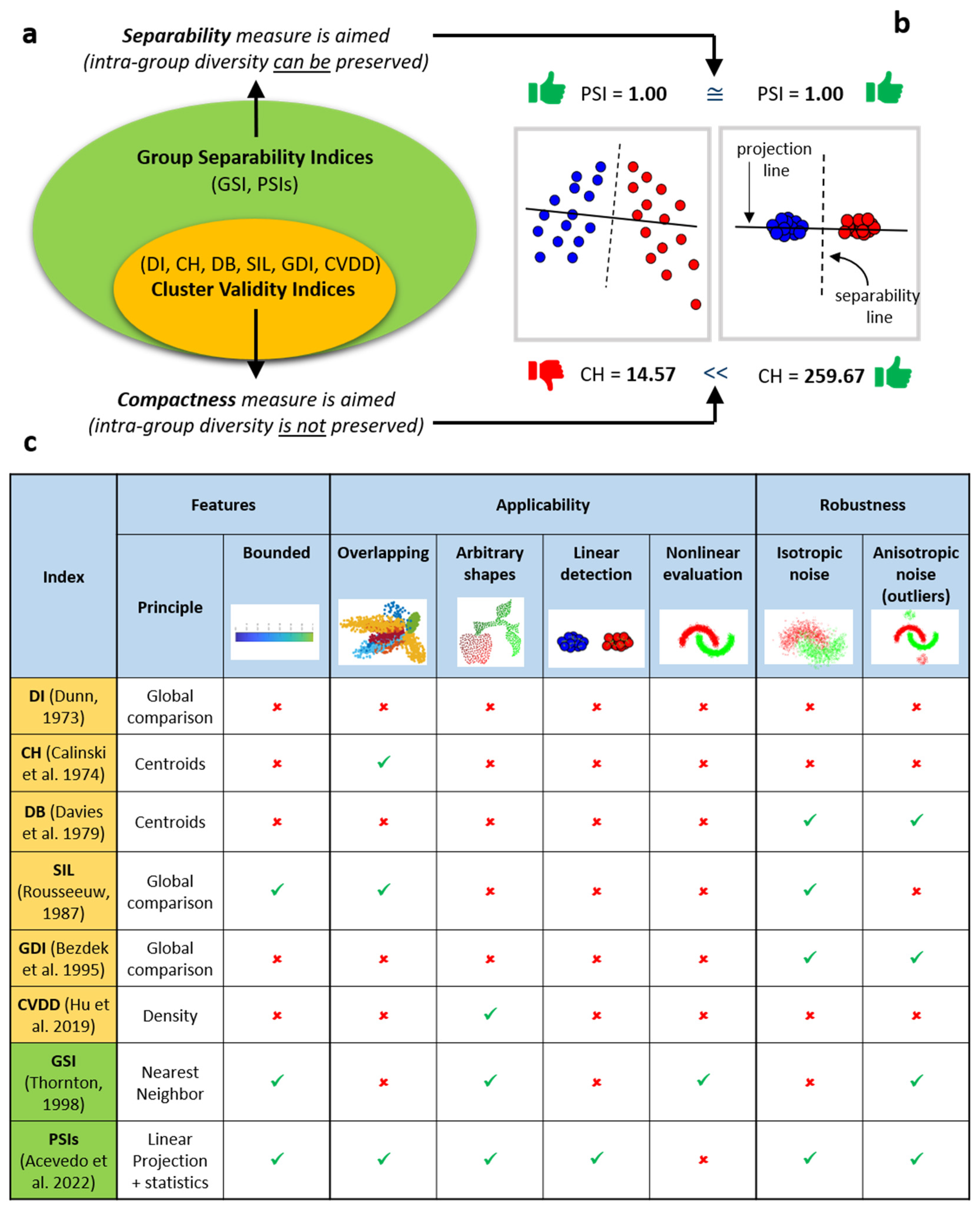
Figure 1. Group separability measures in data science: an overview. (a) Cluster validity indices are a subclass of separability measures that aim to compactness. (b) While group separability measures such as PSI-types aim to preserve both inter- and intra- group diversity rating the same the left and right data representations, a cluster validity measure such as CH rates higher a compact representation that neglects the intra-group diversity. This example offers evidence that using cluster validity indices for evaluation of group separability is not an appropriate solution. (c) Rows indicate different groups separability measures: yellow background for cluster validity measures and green for geometric separability measures. The columns indicate different features of the measure, their applicability to a spectrum of problems that arise in data science, and their robustness under different types of noise.

Figure 4. Statistical significance of the travelling salesman projection separability (TSPS) measure. (a) The travelling salesman (TS) path that connects the points to be rectified (b) and the AUC-PR is computed for assessing the separability of the observed group organization embedded in the geometric space. (c) the labels of the groups are uniformly at random reshuffled and the AUC-PR is computed to generate a random instance. (d) the process to generate random replicates is repeated for a certain number of times (rows, n = 1000 in our study) and for all number of group pairs (columns). (e) Then the mean value across the group pairs (columns) is computed to generate the final value to build a null model distribution. The p-value of the observed TSPS measure is computed as the fraction of random values that are larger than the observed value.

Figure 7. Empirical evidence on real complex multidimensional data. The radar signal dataset is composed of 350 valid samples, 34 features, and three groups: good radar signal, bad radar signal type1 and bad radar signal type2. The complexity of this dataset is associated with the mix of hierarchical and similarity relations between the data samples. (a) Embedding of the radar signal dataset in the two-dimensional space by MCE algorithm. (b) The geometric separability of MCE representation is estimated of high quality (performance larger than 0.8) according to any type of measure, because MCE algorithm is able to produce a representation that accounts for hierarchical structure in the data. (c) t-SNE representation (p = 31 is the best perplexity setting, see text for details) suffers from the crowding problem because t-SNE algorithm does not well preserve hierarchical organization. (d) the geometric separability measures confirm that the representation of t-SNE is of less quality of MCE for what concerns the separability of the data group structure in the representation space. In (b,d) the values of the indices with a significant (p-value < 0.01) geometric separability are marked with a star, which means that these values are very unlikely to be obtained by chance.

Figure 8. The multivariate community separability analysis of the methods performances (MCSAmp). x-axis for PC1 and y-axis for PC2. (a) spots of the same shape represent the same separability measure, spots of the same color represent the same embedding method, the dashed lines of the same color connect the same embedding method evaluated using different separability measures across the networks. Node2vec (green polygon) produces network representations that do not overlap with the ones of other methods. (b) spots of the same shape represent the same embedding method, spots of the same color represent the same separability measure, the dashed lines of the same color connect the same separability measure evaluated on the representations of different embedding methods across the networks. GSI (green triangle) produces separability evaluations that do not overlap with the ones of other measures.

Figure 9. The multivariate community separability analysis of the network representations (MCSAnr). x-axis for PC1 and y-axis for PC2. (a) spots of the same shape represent the same embedding method, spots of the same color represent the same network representation, the dashed lines of the same color connect the same network’s representations evaluated using different separability measures across the networks. (b) adaptive geometric separability (AGS) values evaluated in each network for the three different embedding methods. (c) mean separability of each embedding method across the networks. (d) minimum separability of each embedding method across the networks.

Figure 10. Two-dimensional representations of Football, Polblogs and Karate according to the different embedding methods. x-axis for the first dimension of embedding and y-axis for the second dimension of embedding. The name of the represented network is reported in bold on top of each panel, the name and hyperparameter settings (when available) of the network embedding method are reported under the network name, the adaptive geometric separability (AGS) value together with the name of the separability measure/s that achieved the maximum is reported under the embedding method name.

Disclaimer/Publisher’s Note: The statements, opinions and data contained in all publications are solely those of the individual author(s) and contributor(s) and not of MDPI and/or the editor(s). MDPI and/or the editor(s) disclaim responsibility for any injury to people or property resulting from any ideas, methods, instructions or products referred to in the content.

© 2024 by the authors. Licensee MDPI, Basel, Switzerland. This article is an open access article distributed under the terms and conditions of the Creative Commons Attribution (CC BY) license (http://creativecommons.org/licenses/by/4.0/).

Copyright: This open access article is published under a Creative Commons CC BY 4.0 license, which permit the free download, distribution, and reuse, provided that the author and preprint are cited in any reuse.

MDPI Initiatives

Important Links

Choose an area of interest and we will send you notifications of new preprints at your preferred frequency.

Disclaimer

Geometric Separability of Mesoscale Patterns in Embedding Representation and Visualization of Multidimensional Data and Complex Networks

Abstract

Author Summary

Introduction

Geometric Separability of Mesoscale Patterns in Data Represented in a Two-Dimensional Space

Geometric Separability of Mesoscale Patterns in Complex Networks Represented in a 2D Space

Results

Innovations of This Study

Empirical Evidence on Artificial Datasets and the Adaptive Geometrical Separability (AGS)

Empirical Evidence on Real Complex Multidimensional Data

Empirical Evidence on Real Complex Networks

Discussion

Methods

Data and Algorithms

Synthetic Data Generation

Real Complex Multidimensional Data

Real Complex Networks

Network Embedding Methods

Geometric Separability Indices

Centroid Projection Separability (CPS) and Linear Discriminant Projection Separability (LDPS) Indices

Geometrical Separability Index (GSI)

Travelling Salesman Projection Separability (TSPS)

Statistical Significance of the Geometric Separability Measures

Adaptive Assessment of the Community Separability

Hardware and Software

Data Availability

Code Availability

Author Contributions

Funding

Acknowledgements

Competing Interests

References

MDPI Initiatives

Important Links

Subscribe