
Submitted:
20 June 2024
Posted:
24 June 2024
You are already at the latest version
Abstract
Emerging data processing techniques brought back into attention the HF range communication as an interesting alternative to third-party solutions for IoT applications, such as data transmission in distributed energy production facilities. The physical size of HF antennas, often comparable to the surrounding objects, require in-situ radiation measurements. Drone-borne measuring systems are already known as a flexible solution, but mostly restricted to higher frequency ranges. In this work, we propose to use an electrically small, folded dipole as a probe for drone-borne measurements on HF antennas. We also propose a calibration approach for the effects related to the near-field zone, and to the drone body proximity. The impact of ground reflection is also investigated. We show that despite its low, realized gain figure such a probe can provide stable results for near-field measurements, even at low input power levels.
Keywords:
drone-borne
; HF antennas
; Internet of Things (IoT)
; folded dipole
; Open Area Test Site (OATS)
; antenna measurements
; near-field antenna measurements
1. Introduction
The concept of Internet of Things (IoT) covers communications in distributed energy production facilities, known as smart grid [1], [2]. Communications for transmitting command and control information in smart grid energy facilities should often cover long ranges. As an example, off-shore power plants are often outside of the service area of the mobile networks [3], and satellite communications would be too expensive. Besides, point-to-point communications are always preferred for controls and commands compared to any other third-party solution. Point-to-point solutions in UHF such as LoRa might not be reliable enough, especially in the offshore environment.
Low-power and low-rate HF communication systems [4], [5], can be easily implemented and made extremely reliable for transmitting information through appropriate signal processing [4], [6] and appropriate frequency management [4], [7], [8]. Such communications are not only immune to the noise as they usually operate at a negative signal-to-noise ratio, but they also do not interfere with other communication services due to their extremely low power. Moreover, techniques mainly used for higher frequency ranges such as spread spectrum [9] or ultra-wide band technologies [10] could be implemented on a fully software defined radio platform [11], [12], [13], and can further reduce the risk of interference with other HF communication systems or between components of the same communication system.
The radiation pattern of an HF antenna is highly impacted by the environing objects. In order to provide reliable communications over the entire frequency range of interest between two sites of the grid, the HF antennas should be measured in situ [14], [15], [16], making therefore sure that the main lobe direction is pointing to the correspondent site.
Recently, many drone-borne antenna measuring systems have been developed as drones have become more and more affordable. However, most of those solutions were developed for frequencies above the HF band [16], [17], [18], [19], [20], [21], and very few for HF antennas; the frequencies are mostly above 50 MHz.
It should be emphasized that near-field to far-field transforms must be performed when measuring an HF antenna with a drone-borne system [22], [23].
In this work, we propose a drone-borne data acquisition system using a short, folded dipole as a probe antenna. A calibration procedure to take into account the effect of the drone chassis is also presented.
2. Platform Design
The configuration of the drone-borne antenna measuring system is shown in Figure 1.
When measuring HF antennas with a drone-borne acquisition system, weight and size constraints apply. Most of the commercial-on-the-shelf drones can carry loads of up to 0.5kg, and the load size should not affect the drone stability. As a result, only electrically small probes can be used, such as short straight or folded dipoles, or small loop antennas. Such antennas provide good pattern diagram stability over a wide frequency band; conversely, the radiation resistance is quite low, and the input reactance is high. For HF band measurements non-Foster impedance matching networks can be easily implemented [24], [25], to compensate the antenna input reactance, and the peak detector can be designed as to provide an appropriate input resistance.
Nevertheless, using a non-Foster impedance matching network on a drone-borne system increases power consumption and load mass; besides, exposure to HF radiation might impact on the active circuit operation. A simpler approach would be to terminate the probe on a constant, 50-ohm resistor without using any impedance matching network. In that case, the impedance mismatch loss and the antenna conductor loss might be compensated by reducing the distance to the antenna under test or by increasing the HF transmitter power, though with some precautions regarding the risk of interference with the drone control and communication systems.
3. Probe Design and Calibration
When using a probe antenna on an unmatched impedance termination, the antenna input impedance should be also known, typically by measuring its input reflection coefficient. Calibrating such an antenna also requires gain measurements. Since the antenna will be placed on a metallic drone body, the effect of the drone body should also be investigated.
The two-antenna method [15], [26] can be adapted to characterize such a probe by successively pairing two identical probes as follows: both on dielectric tripods, the first on a dielectric tripod and the second attached to the drone (Figure 2).
The gain can then be found by taking into consideration the input impedance variation,
Since and are not essentially impacted by the drone body proximity it comes out that:
As probes, we considered a pair of 1 m long dipoles (Figure 3); we chose a folded configuration, in order to increase the radiation resistance.
Such a dipole is electrically short over the entire HF band; as a result, the impact of the common mode currents on gain measurements is quite high [27]. One-to-one baluns were used as part of the antenna in order to reduce the effect of the common mode currents and thus, the antennas will be characterized including the transformers. The same balun will be used with the probe on the drone as well.
Gain measurements need to be performed in a reflection free environment; since anechoic chambers for HF antennas are quite rare, we opted for an open area test site (OATS). Reflection and diffraction on massive objects can still occur in that frequency range. The distance averaging method [28], [29] may reduce the effect of the multipath propagation, even for narrow band antenna measurements. Though, for HF antennas it might be unpractical, as the distance variation range between antennas should be in the order of the wavelength to provide sufficient variability to the contribution of the indirect wave. Time gating can be applied instead [30], [31], by correlating the gate width with the distance to the nearest massive obstacle in the OATS.
It should be emphasized that a one meter long, folded dipole acts mostly like an electrically small loop near the lowest limit of the HF range, and as an electrically short dipole, near the highest limit. In-between, both modes of radiation i.e., loop mode and dipole mode are present and comparable. The loop mode (Figure 4a) provides omnidirectional radiation in the antenna plane i.e., YOZ, and a dual polarization, except the XOY plane where solely the Oz polarization is present. The dipole mode provides omnidirectional radiation in the XOY plane (Figure 4b), and a linear polarization along the OZ axis.
Ground reflection effect should be assessed separately by successively placing the antennas in vertical and horizontal positions, in face-to-face and coplanar configurations (Figure 5). Pattern diagrams have 90 degrees wide radiation lobes (half-power beamwidth) both for loop and dipole modes; it is therefore worth to place the antennas one away from the other at a distance twice the mast height, in order to have the same weight in the link budget for the loop mode, ground reflected wave both for coplanar and face-to face configurations. Let R be the ground reflection coefficient; since the distance between antennas and mast height are comparable (i.e., in the order of one meter), and both much less than the wavelengths in the HF range (i.e., tens to one hundred meters) direct and reflected waves are quasi in-phase.
For the horizontal, coplanar configuration the electric field contributing to the current on the receiving antenna can be found as:
where and are the contributions of the dipole mode and loop mode, respectively.
Similarly, for the horizontal, face-to-face configuration one can find:
and
for the vertical, face-to-face configuration.
By subtracting (5) from (4) it comes out that:
and by subtracting (5) from (6).
Next, by adding (5) to (6):
and by substituting in (9) as given in (7) it is found that:
The reflection coefficient can then be computing by dividing (10) by (8),
We denote:
From (11) and (12),
and from (8),
with R calculated as in (13).
Three maximum gain figures can then be defined: the dipole mode gain (corresponding to the ‘face-to-face’ orientation)
the loop mode gain,
and the total gain (corresponding to the ‘coplanar’ orientation),
As the antenna length and the distance between antennas fall in the same order and both are much less than the wavelength it comes out that measurements are performed in the near-field zone. The most important effect compared to a far-field measurement setup comes from the variability of the longitudinal component of the electric field generated by the transmitting antenna, along the receiving antenna (Figure 6).
Let be the output voltage at the receiving antenna. One can define a normalized, received voltage by compensating the effects of propagation in terms of magnitude and phase. By taking into consideration the radiation field into the expression of the mutual impedance for two straight dipoles [32], the normalized received voltage can be written as
Current distributions are assumed to be quasi-constant. Moreover, since r and d are much less than the wavelength the phase of the integrand can be neglected. Given that ,
The far-field received voltage can be found by making d→∞,
A simple correction factor for close-distance transmission between two identical, electrically short dipoles can be found:
Gain measurements in the near-field zone would yield instead of G. The Friis formula for the probe gain should therefore be corrected as follows:
Since computed as before is already a far-field figure the on-drone gain can be found from near-field measurements as
3. Results
3.1. Antenna Input Characteristics
We firstly characterized the balun by measuring its scattering parameters on a standard, 50 ohm normalizing impedance. Based on that, we found the insertion loss of the balun terminated on the folded dipole (Figure 7), and the input impedance both at the antenna input and at the balun input.
Figure 8 shows the variation as a function of frequency of the resistance, reactance, and VSWR at the antenna input. Losses in the antenna wire and balun make it possible to get a VSWR mostly below five over the frequency range of interest i.e., between 7 and 30 MHz. The efficiency ranges between −36 and −7.8dB; however, our gain measurements yield stable results for transmission between two such antennas placed at distances of up to 2.5 meters one from the other, and for an input power of 0 dBm.
3.2. Ground Reflection
All antenna measurements were performed in an open area test site (OATS) i.e., on a beach after more than 15 rainless days. The calibration of the electrically short dipole configuration to be installed on the drone was performed through S-parameters measurements between two identical antennas, including baluns.
The antennas were placed at 2.5 m away one from the other, face-to-face, in horizontal and vertical position, respectively (Figure 9). Both tripods were adjusted at a height of 1.25 m.
Dipole mode and loop mode gain figures were computed by using (15) and (16) and shown in Figure 10.
The ground reflection coefficient (Figure 11a) and the gain figures corrected for ground reflection (Figure 11b and c) were computed by using (13), (15), and (17).
It comes out that ground reflection in the current measuring site does not critically impact on the accuracy, which is slightly better for a ‘face-to-face’ orientation.
3.3. Probe Calibration with Field-Zone Correction and On-Drone Measurements
Two identical, electrically small dipoles were placed in horizontal, face-to-face position at 0.5, 1, 1.5, 2, and 2.5 m away one from the other. One of the antennas was placed at first off-drone (Figure 12a) and then on-drone (Figure 12b).
The gain variation over the HF range with and without field zone correction by using (2) and (23) is given in Figure 13.
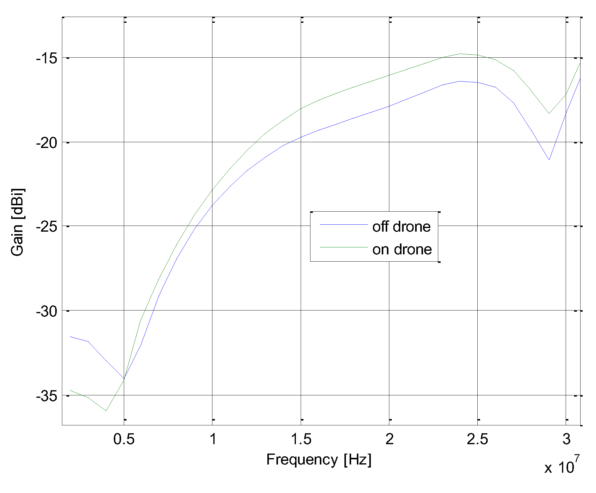
Figure 14 depicts a gain comparison for the on drone and off-drone configurations.
4. Conclusions
In this work, we proposed to use an electrically small, folded dipole as a probe for in-situ drone-borne gain measurements on HF antennas. We presented a calibration procedure taking into account the effect of the field zone, ground reflection, and drone body proximity.
Regarding the design, it comes out that losses in the antenna wire and balun rather have a positive impact, as the VSWR is less than five over the entire frequency band of interest i.e., between, 7 and 30 MHz. The realized gain exhibits a smooth variation between −25 and −15dBi; transmission measurements between two identical folded dipoles show that such low gain figures provide stable and noiseless results at distances of up to 2.5 meters between antennas even at an input power in the order of 1 mW.
The dipole-type radiation mode dominates over the loop-type mode over the frequency range of interest, and the impact of the ground reflection is mostly less than 1dB for a face-to-face orientation.
Our calibration procedure helps to improve the accuracy of gain measurement of up to 4dB for the field-zone related discrepancies, and by around 2dB for the drone body impact.
Author Contributions
Conceptualization, M.P., A.C., A.H. and R.D.T.; methodology, M.P., A.C., A.H. and R.D.T.; software, M.P. and R.D.T.; validation, M.P., A.C., A.H. and R.D.T.; formal analysis, M.P., A.C., A.H. and R.D.T.; investigation, M.P., A.C., A.H. and R.D.T.; resources, R.D.T.; data curation, M.P., A.C., A.H. and R.D.T.; writing—original draft preparation, M.P., A.C., A.H. and R.D.T.; writing—review and editing, R.D.T.; visualization, M.P., A.C., A.H. and R.D.T.; supervision, R.D.T.; project administration, R.D.T.; funding acquisition, R.D.T. All authors have read and agreed to the published version of the manuscript.
Funding
This work was supported under the project MAREHC, a grant of the Romanian Ministry of Research, Innovation and Digitalization, project number PNRR-C9-I8-760111/23.05.2023, code CF 48/14.11.2022, within PNRR.
Data Availability Statement
Ongoing research project requiring confidential data status.
Conflicts of Interest
The authors declare no conflict of interest.
References
- C. P. Ohanu, S. A. Rufai, and U. C. Oluchi, “A comprehensive review of recent developments in smart grid through renewable energy resources integration,” Heliyon, vol. 10, no. 3, p. e25705, Feb. 2024. [CrossRef]
- M. J. B. Kabeyi and O. A. Olanrewaju, “Smart grid technologies and application in the sustainable energy transition: a review,” International Journal of Sustainable Energy, vol. 42, no. 1, pp. 685–758, Dec. 2023. [CrossRef]
- Z. Zhang, T. Peng, K. Yang, and X. Li, “Trajectory Optimization and Retrieving Monitory System for UAV-assisted Offshore Maritime Communications,” in 2023 3rd International Conference on Electronic Information Engineering and Computer Science (EIECS), Sep. 2023, pp. 1014–1019. [CrossRef]
- T. Koziniec, D. Murray, and M. Dixon, “Precomputed Ionospheric Propagation for HF Wireless Sensor Transmission Scheduling,” in 2021 29th International Symposium on Modeling, Analysis, and Simulation of Computer and Telecommunication Systems (MASCOTS), Nov. 2021, pp. 1–8. [CrossRef]
- P. Marti-Puig, M. Serra-Serra, and R. Reig Bolaño, “Low complex wireless sensor network uplink in the HF band,” Apr. 2008, Accessed: Jun. 03, 2024. [Online]. Available: https://upcommons.upc.edu/handle/2099/4925.
- “WSJT-X User Guide.” Accessed: Mar. 14, 2024. [Online]. Available: https://wsjt.sourceforge.io/wsjtx-doc/wsjtx-main-2.6.1.html.
- W. A. Parkins, “Propagation management for no-acknowledge HF communications links,” 1986. Accessed: Mar. 14, 2024. [Online]. Available: https://ui.adsabs.harvard.edu/abs/1986MsT..........5P.
- “HF_radio_GM _ISPACG_Ver1.pdf.” Accessed: May 23, 2024. [Online]. Available: https://www.icao.int/APAC/documents/edocs/cns/HF_radio_GM%20_ISPACG_Ver1.pdf.
- X. Tan, S. Su, and X. Sun, “Research on Narrowband Interference Suppression Technology of UAV Network Based on Spread Spectrum Communication,” in 2020 IEEE International Conference on Artificial Intelligence and Information Systems (ICAIIS), Mar. 2020, pp. 335–338. [CrossRef]
- R. D. Tamas, L. Babour, E. Fond, G. Slamnoiu, J. Chilo, and P. Saguet, “Cylindrical dipoles as ultra-wide band antennas: An energy-based analysis,” Microwave and Optical Technology Letters, vol. 50, no. 4, pp. 917–921, 2008. [CrossRef]
- S. M. Bostan, J. V. Urbina, J. D. Mathews, S. G. Bilén, and J. K. Breakall, “An HF Software-Defined Radar to Study the Ionosphere,” Radio Science, vol. 54, no. 9, pp. 839–849, 2019. [CrossRef]
- Wicaksono, A. Mauludiyanto, and G. Hendrantoro, “An HF Digital Communication System Based on Software-Defined Radio,” in 2020 International Conference on Smart Technology and Applications (ICoSTA), Feb. 2020, pp. 1–5. [CrossRef]
- R. R. Belgibaev, V. A. Ivanov, D. V. Ivanov, and A. R. Laschevsky, “Software-Defined Radio Ionosonde for Diagnostics of Wideband HF Channels with the Use of USRP Platform,” in 2019 Wave Electronics and its Application in Information and Telecommunication Systems (WECONF), Jun. 2019, pp. 1–4. [CrossRef]
- “IEEE Recommended Practice for Antenna Measurements,” IEEE Std 149-2021 (Revision of IEEE Std 149-1977), pp. 1–207, Feb. 2022. [CrossRef]
- “IEEE Standard Test Procedures for Antennas,” ANSI/IEEE Std 149-1979, pp. 1–144, Nov. 1979. [CrossRef]
- Y. Alvarez et al., “In situ antenna diagnostics and characterization system based on RFID and Remotely Piloted Aircrafts,” Sensors and Actuators A: Physical, vol. 269, Nov. 2017. [CrossRef]
- P. Bolli et al., “Antenna pattern characterization of the low-frequency receptor of LOFAR by means of an UAV-mounted artificial test source,” presented at the SPIE Astronomical Telescopes + Instrumentation, H. J. Hall, R. Gilmozzi, and H. K. Marshall, Eds., Edinburgh, United Kingdom, Jul. 2016, p. 99063V. [CrossRef]
- F. Paonessa et al., “UAV-based pattern measurement of the SKALA,” in 2015 IEEE International Symposium on Antennas and Propagation & USNC/URSI National Radio Science Meeting, Jul. 2015, pp. 1372–1373. [CrossRef]
- E. de Lera Acedo et al., “SKA aperture array verification system: electromagnetic modeling and beam pattern measurements using a micro UAV,” Exp Astron, vol. 45, no. 1, pp. 1–20, Mar 2018. [CrossRef]
- G. Virone et al., “Antenna Pattern Verification System Based on a Micro Unmanned Aerial Vehicle (UAV),” IEEE Antennas and Wireless Propagation Letters, vol. 13, pp. 169–172, 2014. [CrossRef]
- P. Bolli et al., “In-situ characterization of international low-frequency aperture arrays by means of an UAV-based system,” in 2017 XXXIInd General Assembly and Scientific Symposium of the International Union of Radio Science (URSI GASS), Montreal, QC: IEEE, Aug. 2017, pp. 1–4. [CrossRef]
- C. Apriono, Nofrizal, M. Dandy Firmansyah, F. Y. Zulkifli, and E. T. Rahardjo, “Near-field to far-field transformation of cylindrical scanning antenna measurement using two dimension fast-fourier transform,” in 2017 15th International Conference on Quality in Research (QiR) : International Symposium on Electrical and Computer Engineering, Jul. 2017, pp. 368–371. [CrossRef]
- F. M. E. Camilo, C. G. do Rego, and G. L. Ramos, “Near-to-far-field transform sample reduction through statistical analysis,” in 12th European Conference on Antennas and Propagation (EuCAP 2018), Apr. 2018, pp. 1–4. [CrossRef]
- M.-C. Tang, T. Shi, and R. W. Ziolkowski, “Electrically Small, Broadside Radiating Huygens Source Antenna Augmented With Internal Non-Foster Elements to Increase Its Bandwidth,” IEEE Antennas and Wireless Propagation Letters, vol. 16, pp. 712–715, 2017. [CrossRef]
- R. W. Ziolkowski and N. Zhu, “Broad bandwidth, efficient, metamaterial-inspired, electrically small antennas augmented with internal non-Foster elements,” in 2012 6th European Conference on Antennas and Propagation (EUCAP), Mar. 2012, pp. 123–125. [CrossRef]
- K. K. Mistry, P. I. Lazaridis, Z. D. Zaharis, M. Akinsolu, Bo Liu, and Tian Loh, “Accurate antenna gain estimation using the two-antenna method,” in Antennas and Propagation Conference 2019 (APC-2019), Birmingham, UK: Institution of Engineering and Technology, 2019, p. 4 pp.-4 pp. [CrossRef]
- Constantin and R. D. Tamas, “Evaluation and Impact Reduction of Common Mode Currents on Antenna Feeders in Radiation Measurements,” Sensors, vol. 20, no. 14, Art. no. 14, Jan 2020. [CrossRef]
- R. D. Tamas, D. Deacu, G. Caruntu, and T. Petrescu, “An indoor measuring technique for antenna gain,” in 2013 International Workshop on Antenna Technology (iWAT), Mar. 2013, pp. 219–222. [CrossRef]
- R. D. Tamas, L. Babour, A. Danisor, and G. Caruntu, “An intermediate-field approach of the differential time-domain single-antenna method for electrically large ultra-wide band antennas,” in 2010 International Workshop on Antenna Technology (iWAT), Mar. 2010, pp. 1–4. [CrossRef]
- Y.-T. Hsiao, Y.-Y. Lin, Y.-C. Lu, and H.-T. Chou, “Applications of time-gating method to improve the measurement accuracy of antenna radiation inside an anechoic chamber,” in IEEE Antennas and Propagation Society International Symposium. Digest. Held in conjunction with: USNC/CNC/URSI North American Radio Sci. Meeting (Cat. No.03CH37450), Jun. 2003, pp. 794–797 vol.3. [CrossRef]
- Constantin, L. Anchidin, and R. D. Tamas, “A Distance Averaging Approach for Measuring the Radiation from Common Mode Currents on Antenna Feeders,” in 2020 International Workshop on Antenna Technology (iWAT), Feb. 2020, pp. 1–4. [CrossRef]
- J. Richmond and N. Geary, “Mutual impedance of nonplanar-skew sinusoidal dipoles,” IEEE Transactions on Antennas and Propagation, vol. 23, no. 3, pp. . 412–414, May 1975. [CrossRef]
Figure 1.
Drone-borne antenna measuring system.
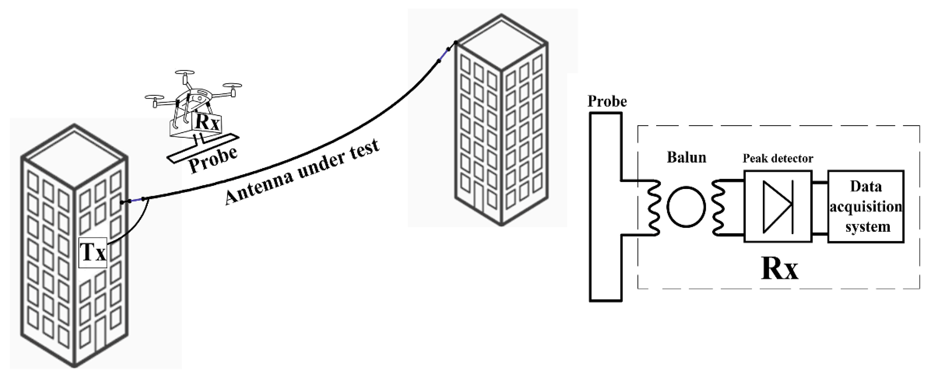
Figure 2.
Two-antenna method for drone-borne probe calibration: (a) off-drone; (b) on-drone measurements.
Figure 2.
Two-antenna method for drone-borne probe calibration: (a) off-drone; (b) on-drone measurements.

Figure 3.
Folded dipole as a probe.
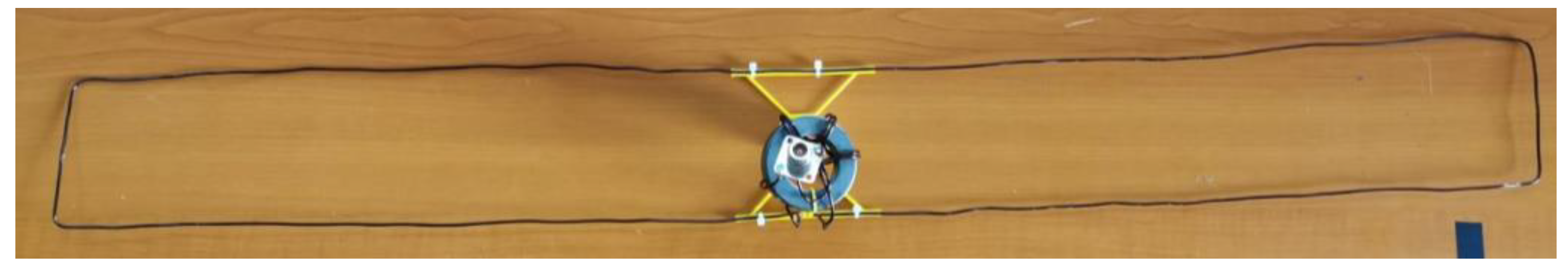
Figure 4.
Radiation from a short, folded dipole: (a) loop mode; (b) dipole mode.
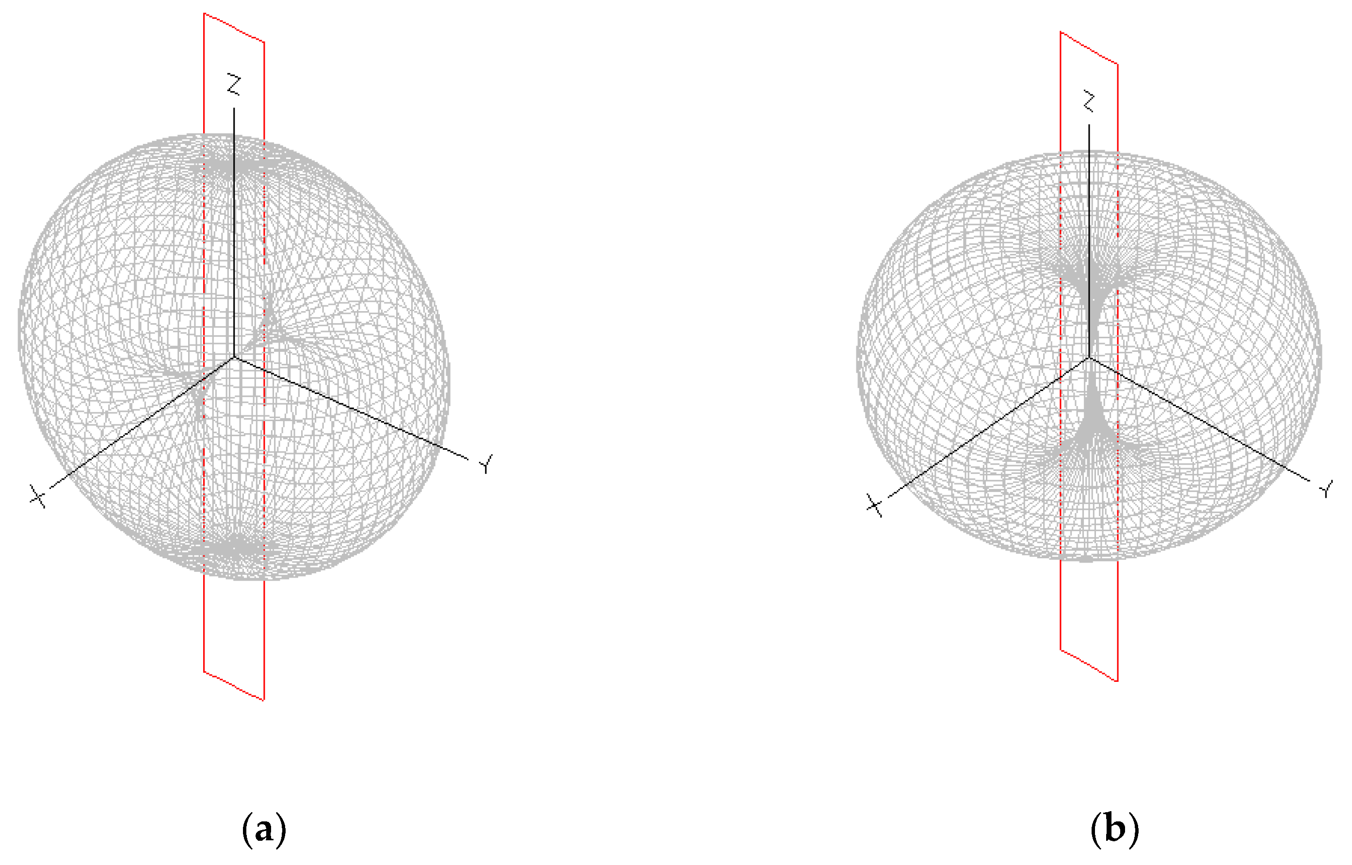
Figure 5.
Evaluation of the ground reflection effect: (a) horizontal, coplanar configuration; (b) horizontal, face-to-face configuration; (c) vertical face-to-face configuration.
Figure 5.
Evaluation of the ground reflection effect: (a) horizontal, coplanar configuration; (b) horizontal, face-to-face configuration; (c) vertical face-to-face configuration.
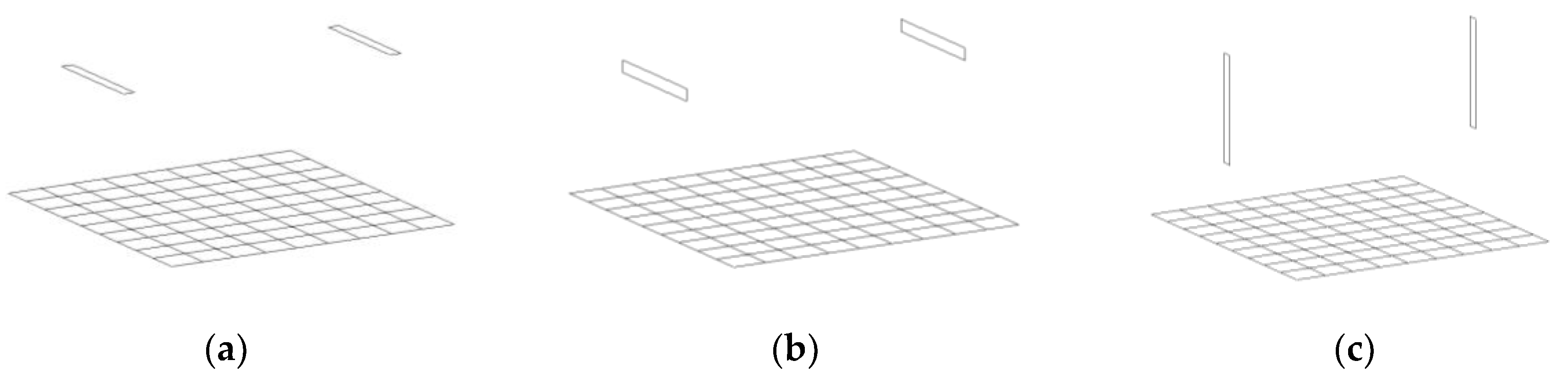
Figure 6.
Near field transmission between electrically short dipoles.

Figure 7.
Insertion loss of the balun terminated on the folded dipole.
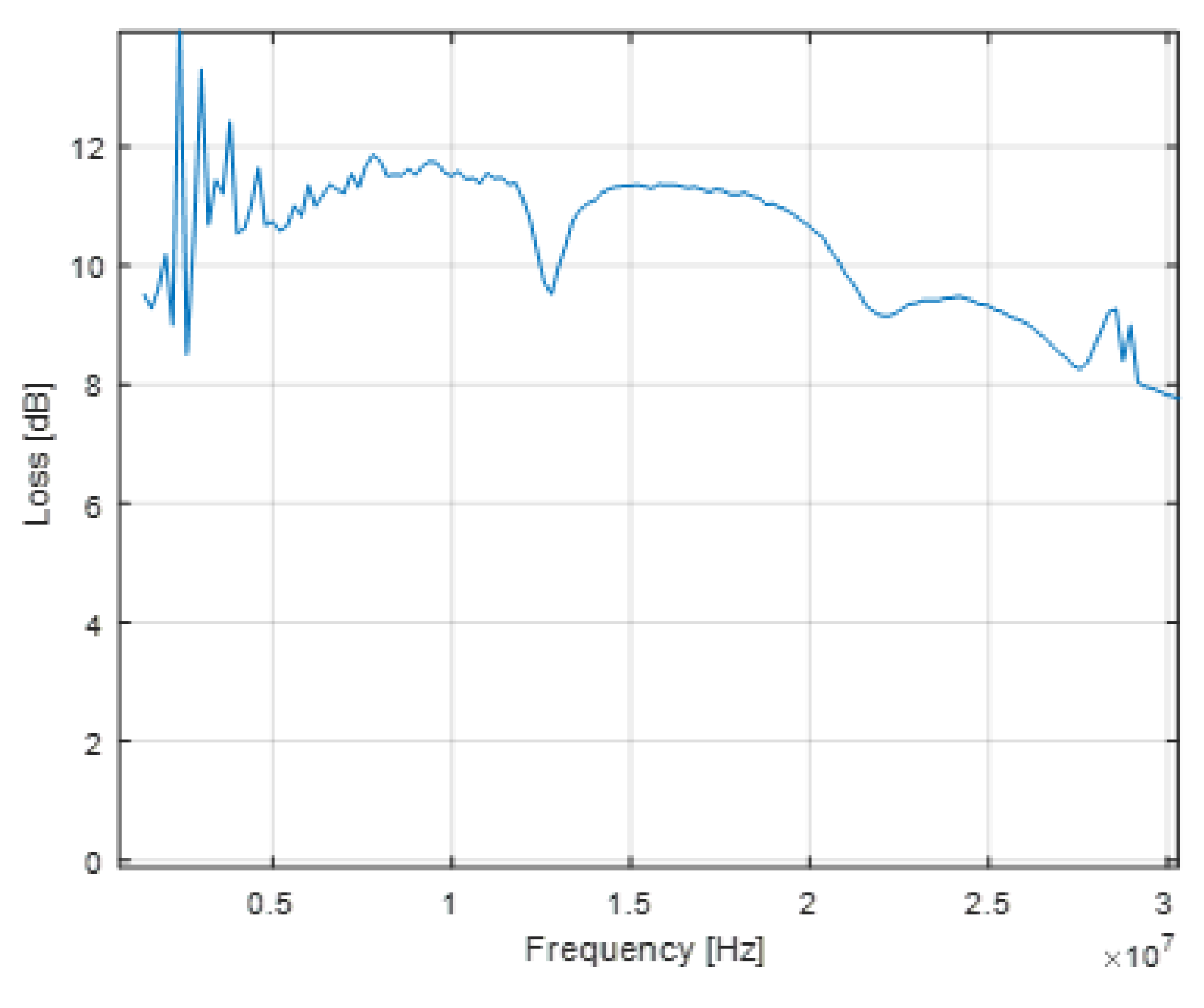
Figure 8.
Antenna input characteristics, with and without balun: (a) resistance; (b) reactance; (c) VSWR.
Figure 8.
Antenna input characteristics, with and without balun: (a) resistance; (b) reactance; (c) VSWR.
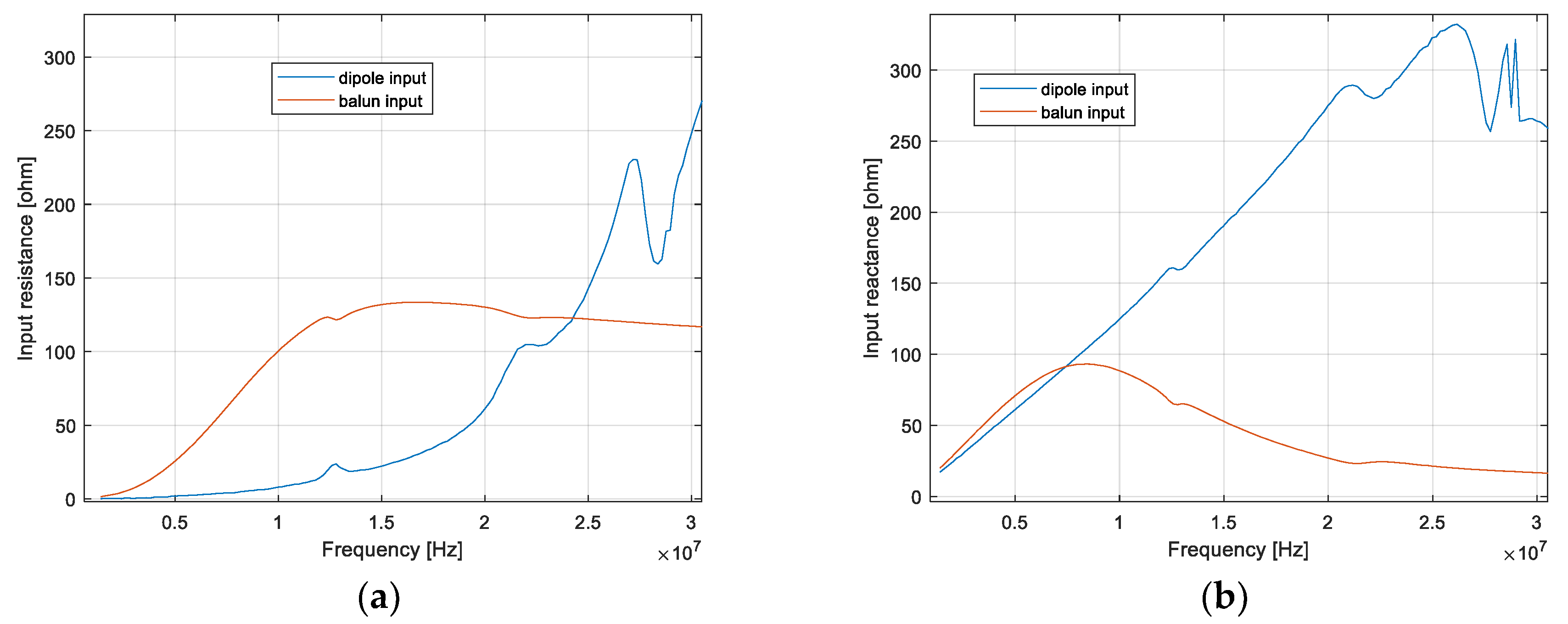
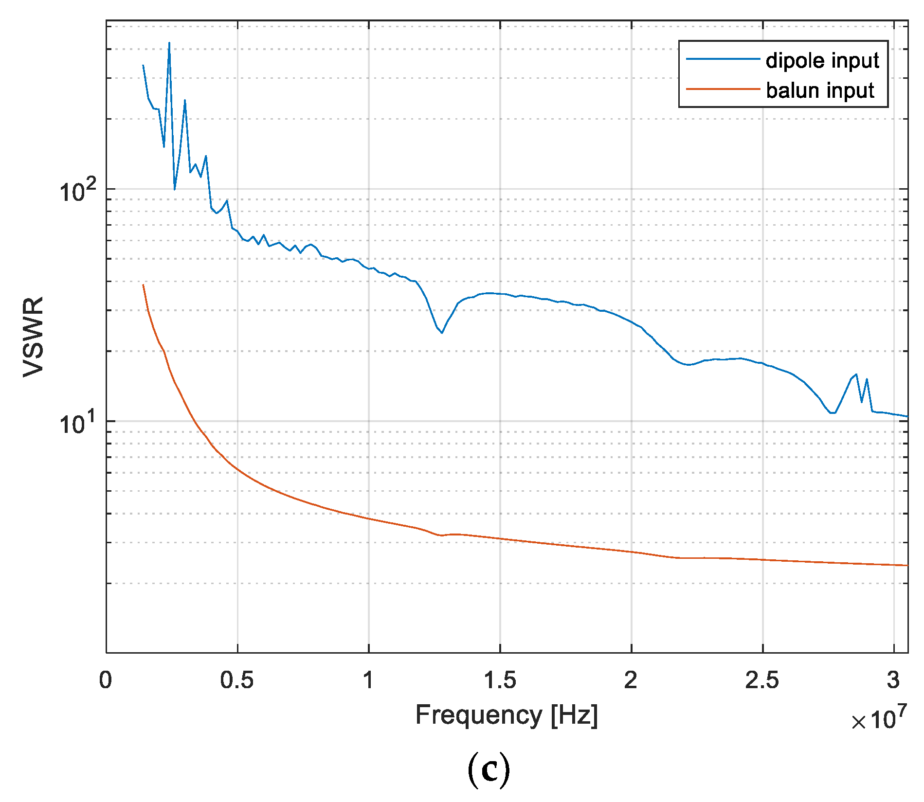
Figure 9.
Antenna setup for ground reflection measurements in an OATS: (a) horizontal, coplanar orientation; (b) horizontal, face-to-face; (c) vertical, face-to-face.
Figure 9.
Antenna setup for ground reflection measurements in an OATS: (a) horizontal, coplanar orientation; (b) horizontal, face-to-face; (c) vertical, face-to-face.

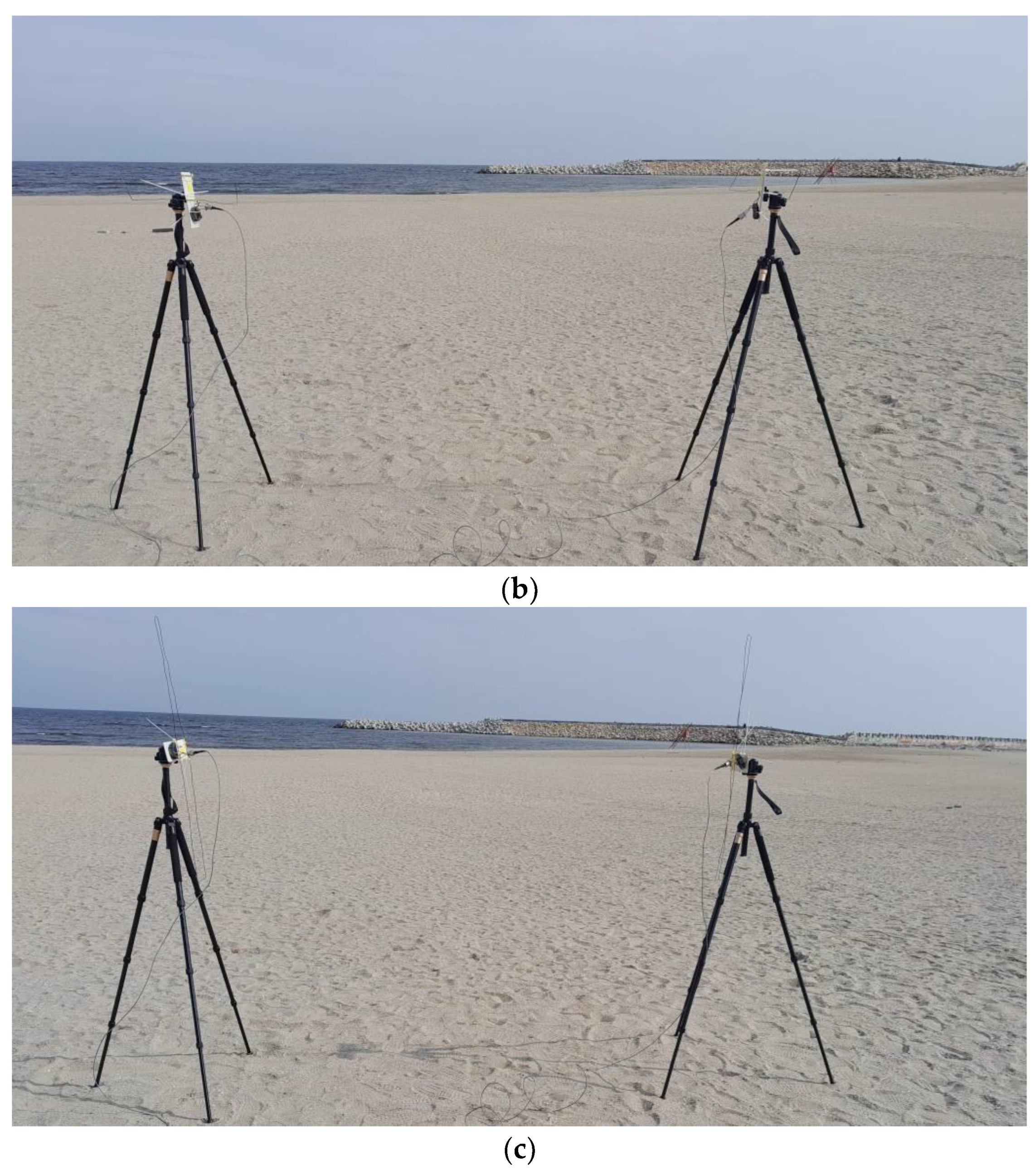
Figure 10.
Gain: (a) dipole mode; (b) loop mode.
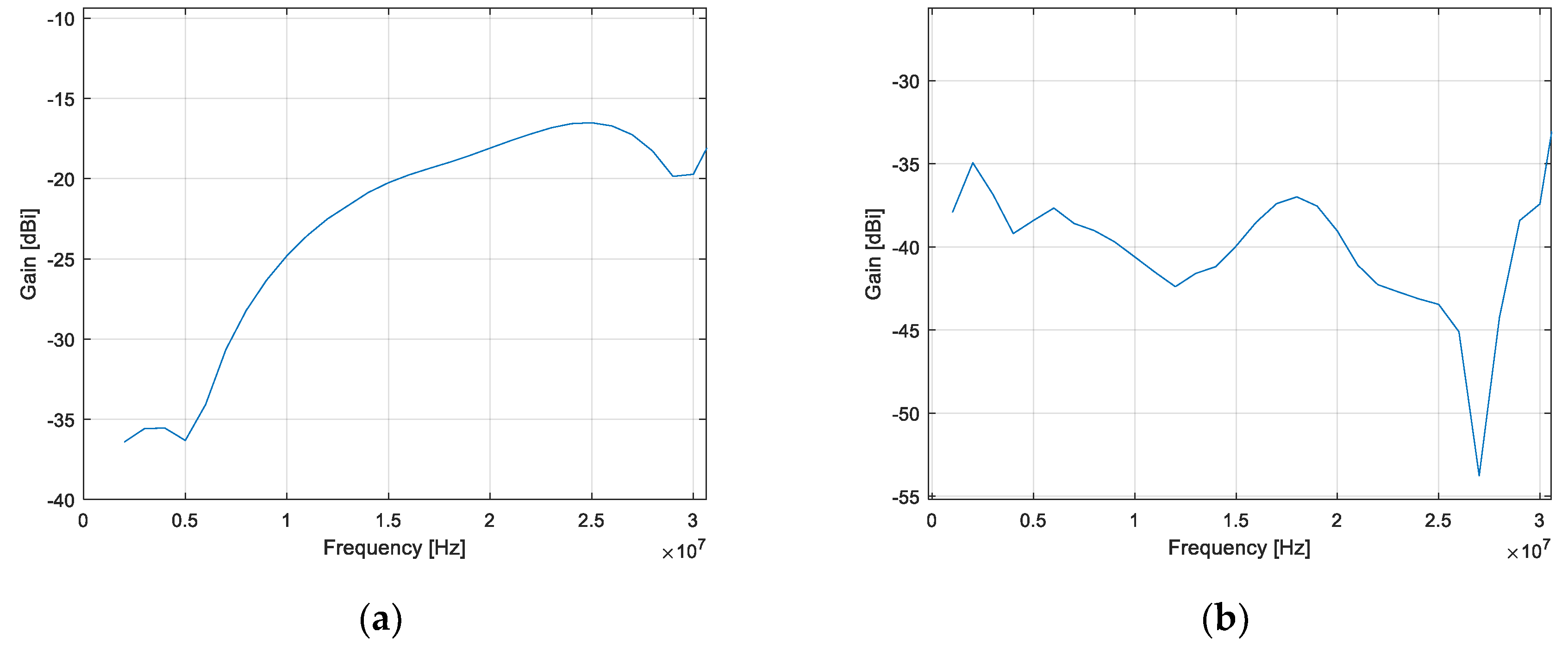
Figure 11.
Ground effect: (a) Ground reflection coefficient; (b) gain: horizontal, ‘face-to-face’ orientation, with and without ground reflection correction; (c) gain: horizontal, ‘coplanar’ orientation, with and without ground reflection correction.
Figure 11.
Ground effect: (a) Ground reflection coefficient; (b) gain: horizontal, ‘face-to-face’ orientation, with and without ground reflection correction; (c) gain: horizontal, ‘coplanar’ orientation, with and without ground reflection correction.
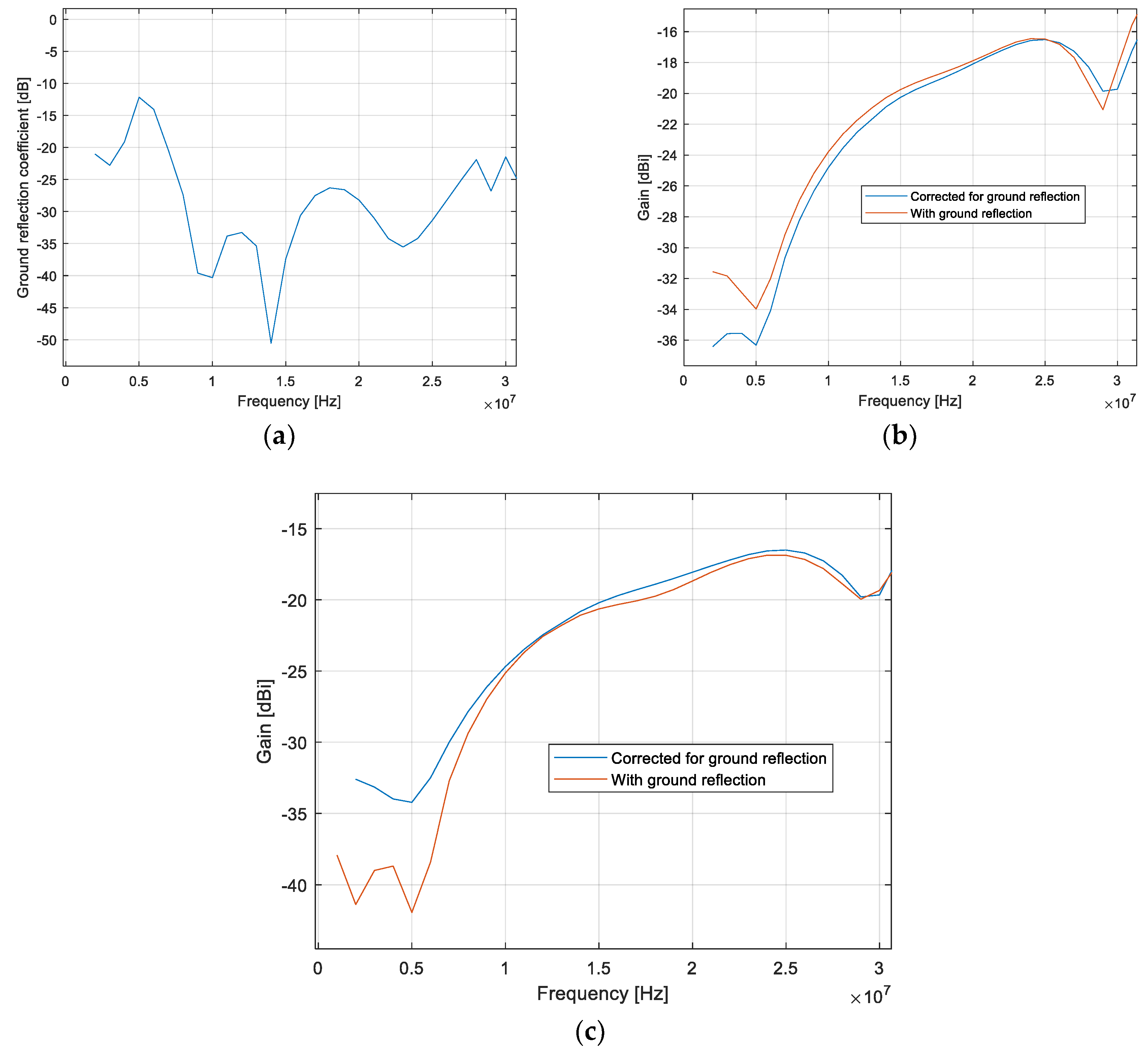
Figure 12.
Antenna setup for on-drone gain measurements in an OATS: (a) horizontal, off-drone face to face antennas as a reference; (b) horizontal, on-drone face to face antennas.
Figure 12.
Antenna setup for on-drone gain measurements in an OATS: (a) horizontal, off-drone face to face antennas as a reference; (b) horizontal, on-drone face to face antennas.
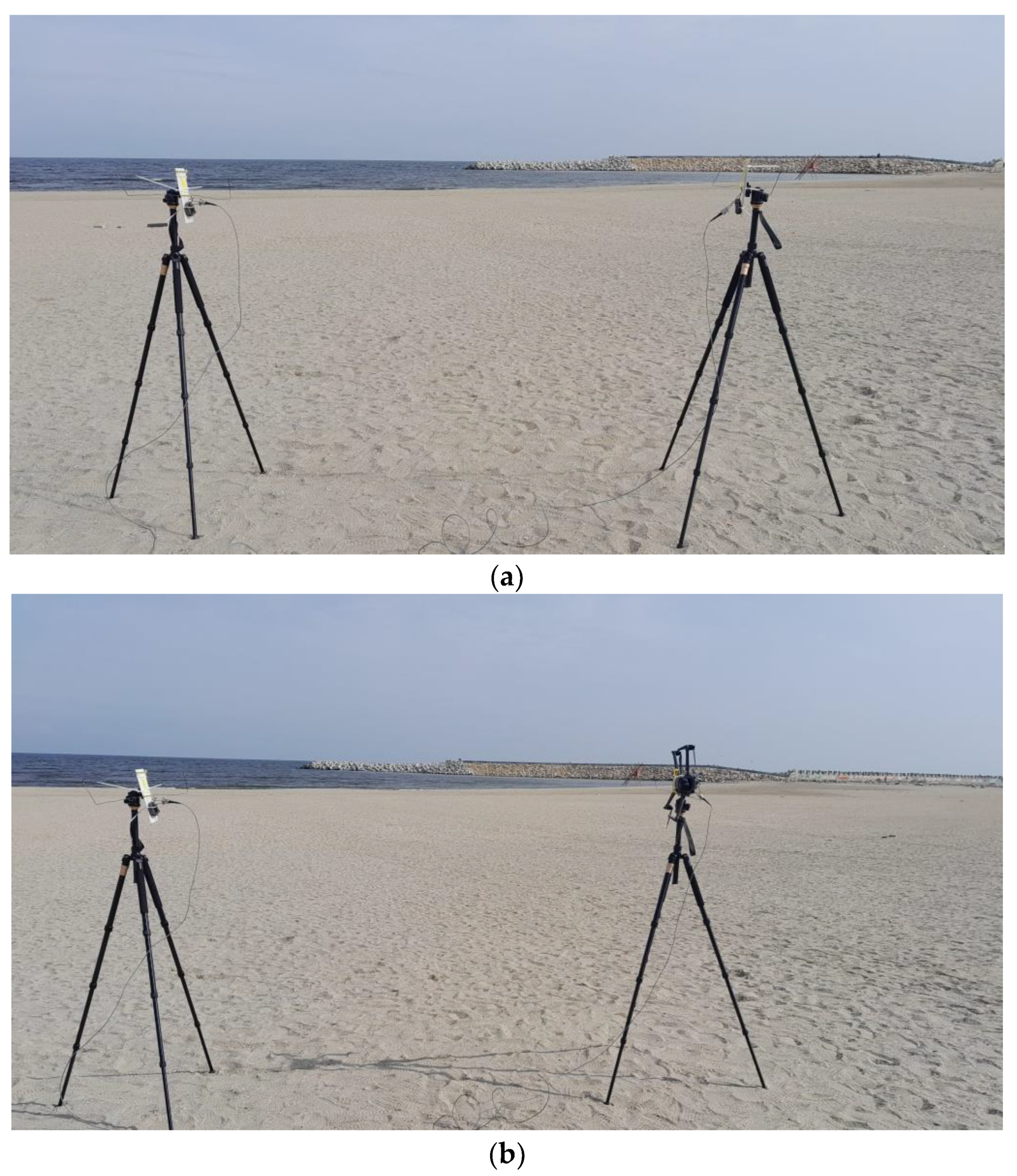
Figure 13.
Gain variation over the HF range: (a)without field zone correction; (b) with field zone correction.
Figure 13.
Gain variation over the HF range: (a)without field zone correction; (b) with field zone correction.
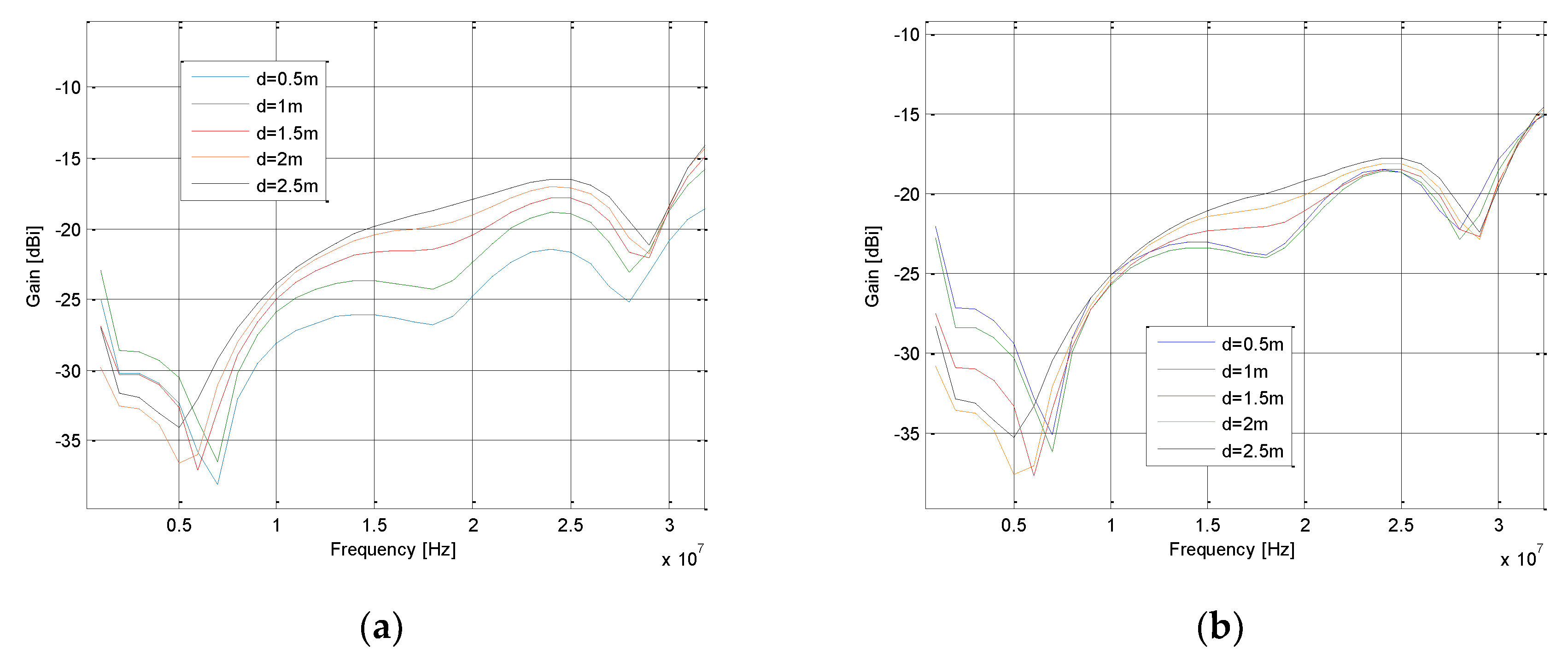
Figure 14.
On-drone versus off-drone gain.
Disclaimer/Publisher’s Note: The statements, opinions and data contained in all publications are solely those of the individual author(s) and contributor(s) and not of MDPI and/or the editor(s). MDPI and/or the editor(s) disclaim responsibility for any injury to people or property resulting from any ideas, methods, instructions or products referred to in the content. |
© 2024 by the authors. Licensee MDPI, Basel, Switzerland. This article is an open access article distributed under the terms and conditions of the Creative Commons Attribution (CC BY) license (http://creativecommons.org/licenses/by/4.0/).
Copyright: This open access article is published under a Creative Commons CC BY 4.0 license, which permit the free download, distribution, and reuse, provided that the author and preprint are cited in any reuse.


