Time Series Forecasting with Many Predictors

Preprint

Article

Time Series Forecasting with Many Predictors

Altmetrics

Downloads

Views

Comments

A peer-reviewed article of this preprint also exists.

This version is not peer-reviewed

Submitted:

13 June 2024

Posted:

21 June 2024

You are already at the latest version

Alerts

Abstract

We propose a novel approach for time series forecasting with many predictors, referred to as the GO-sdPCA, in this paper. The approach employs a variable selection method known as the group orthogonal greedy algorithm and the high-dimensional Akaike information criterion to mitigate the impact of irrelevant predictors. Moreover, a novel technique, called peeling, is used to boost the variable selection procedure so that many factor-relevant predictors can be included in prediction. Finally, the supervised dynamic principal component analysis (sdPCA) method is adopted to account for the dynamic information in factor recovery. In simulation studies, we found that the proposed method adapts well to unknown degrees of sparsity and factor strength, which results in good performance even when the number of relevant predictors is large compared to the sample size. Applying to economic and environmental studies, the proposed method consistently performs well compared to some commonly used benchmarks in one-step-ahead out-sample forecasts.

Keywords:

Subject: Business, Economics and Management - Econometrics and Statistics

MSC: 62M10; 62M20; 62J05

1. Introduction

In the current data-rich environment, many predictors are often available in time series forecasting. However, conventional methods have encountered serious difficulties in exploiting the information contained in such high-dimensional data. In particular, the curse of dimensionality often leads to unreliable forecasts when the conventional methods are applied naively. To exploit the information in the high-dimensional predictors, the use of latent factors has emerged among the first successful approaches. See, for instance, Pena and Box [1], Stock and Watson [2,3], Lam et al. [4], and Chapter 6 of Tsay [5]. These factor-based methods are also widely used in the econometric analysis of high-dimensional time series [e.g. 6,7,8,9].

Nevertheless, existing factor-based methods may still be inadequate, and several issues have been constantly observed in practice. For example, weak factors are prevalent in real-world data and extracting factors using all predictors may not be optimal [10]. In addition, some factor models may still contain many parameters when the factor dimension is not small. On the other hand, Kim and Swanson [11] reported, from an extensive experiment, that combining shrinkage methods with factor-based approaches can yield more accurate forecasts among many targeted macroeconomic time series. This implies that there might exist some irrelevant predictors in an empirical application. The recently proposed scaled principal component analysis of Huang et al. [12] and the supervised dynamic PCA (sdPCA) of Gao and Tsay [13] partially remedy this issue by constructing factors in a supervised fashion, so that the effects of irrelevant predictors are reduced. Limited experience indicates that when the number of predictors far exceed the sample size or when the predictors are highly correlated, the performance of such supervised approaches can still be compromised.

To efficiently extract predictive factors from high-dimensional data, in this paper, we propose a new method that blends variable selection in factor estimation. The proposed method uses the group orthogonal greedy algorithm (GOGA, Chan et al. 14) to screen variables that are relevant to the prediction problem at hand, and apply the sdPCA of Gao and Tsay [13] to extract factors from the selected variables. The orthogonal greedy algorithm, as well as its variant GOGA for grouped predictors, have been employed for variable selection for high-dimensional linear models, especially with dependent data and highly correlated predictors [14,15,16]. Since both GOGA and sdPCA serve to minimize the effects of noisy irrelevant variables, the combined procedure, which we call GO-sdPCA, can effectively construct highly predictive factors.

It is worth pointing out that the novelty of our method lies in a key step that successfully combines variable selection with factor-based methods. Indeed, variable selection techniques commonly employed such as the Lasso of Tibshirani [17] or the OGA of Ing and Lai [16] tend to select a sparse representation of the data. These methods will select only a few variables when many variables are driven by common factors and thereby highly correlated. For factor estimation, this can be undesirable since factor recovery typically benefits from the many variables that are loaded on the shared factors [see, e.g. [4,13]. This issue can be even more pronounced when the factors are strong, in which case the factors can be accurately recovered by employing many predictors. To circumvent this predicament, we propose to use a “peeling” technique, which repeatedly apply GOGA to the data after previously selected variables are dropped from the set of candidate predictors. In this way, our method can select more variables in the model and discriminate between relevant and irrelevant predictors. In Section 4, we intoduce the proposed method in more details. To better motivate the proposed method, we briefly review the orthogonal greedy algorithm (OGA) and its variants in Section 2. We also review the high-dimensional information criteria that are often used to balance the model complexity and the model fit along OGA iterations. The sdPCA is reviewed in Section 3, where we particularly emphasize the method’s design principles.

We use simulation studies and some empirical analyses to examine the performance of the proposed GO-sdPCA approach. In addition to comparing with some factor-based methods, such as the diffusion index approach of Stock and Watson [2,3], the sdPCA, and the time series factor model of Lam et al. [4], we also compare GO-sdPCA against the Lasso and the random forests of Breiman [18], both of which are widely-used and versatile tools in machine learning. We found that GO-sdPCA improves upon most of factor-based approaches and fares well with selected competing methods, even when the number of relevant variables is comparable with the sample size. The simulation results are discussed in Section 5.

In Section 6, we apply the proposed method to two real datasets. The first dataset is the well-known FRED-MD macroeconomic data [9]. Time series forecasting has been a vital topic both in econometric research and in policy-making pertaining to this data set. The other dataset contains the hourly particulate matters (PM_2.5) measurements in Taiwan. The PM_2.5 data play an important role in the environmental studies as well as informing public health policies. However, since its measurements are taken over time and space, the dataset is naturally of high dimension and presents serious challenges to forecast. Our findings demonstrate that the proposed method consistently offers more accurate forecasts than the competing methods, validating its practical utility.

2. Orthogonal Greedy Algorithm

In this section, we briefly review the (group) orthogonal greedy algorithm. The OGA is an iterative algorithm that sequentially chooses predictors to form a regression model. Theoretically grounded in approximation theory [19], the OGA is also easy to implement computationally. In the statistical learning and high-dimensional linear regression literature, Barron et al. [20] and Ing and Lai [16] analyzed its convergence rate as well as variable screening capability. Its generalization to grouped predictors was studied by Chan et al. [14] with application to threshold autoregressive time series models.

Throughout this paper, we denote by

y = {(y_{1}, \dots, y_{n})}^{⊤}

the data of the response variable we are interested in, where n is the sample size. We also have data for the p predictors,

{x_{(j)} : j = 1, 2, \dots, p}

, where

x_{(j)} = {(x_{1, j}, \dots, x_{n, j})}^{⊤}

. The OGA is defined as follows. Starting with

{\hat{J}}_{0} = \emptyset

and

u^{(0)} = y = {(y_{1}, y_{2}, \dots, y_{n})}^{⊤}

, the OGA computes, at iteration

k = 1, 2, \dots

\begin{matrix} {\hat{j}}_{k} & = arg min_{1 \leq j \leq p} {∥ u^{(k - 1)} - x_{(j)} {(x_{(j)}^{⊤} x_{(j)})}^{- 1} x_{(j)}^{⊤} u^{(k - 1)} ∥}^{2}, \end{matrix}

(1)

and updates

\begin{matrix} {\hat{J}}_{k} & = {\hat{J}}_{k - 1} \cup {{\hat{j}}_{k}}, \\ u^{(k)} & = (I - H_{(k)}) y . \end{matrix}

where

H_{(k)}

is the orthogonal projection matrix associated with the linear space spanned by

{x_{(j)} : j \in {\hat{J}}_{k}}

. Clearly, the OGA sequentially selects variable to include in the model; the set

{\hat{J}}_{k}

denotes the index set corresponding to the predictors already selected at iteration k. Intuitively, in each iteration OGA selects the variable that best explains the current residuals. There are numerical schemes to speed up the computation of the residuals such as using sequential orthogonalization. We refer to Ing and Lai [16] and Chan et al. [14] for details.

For the purpose of this paper, we will make use of a slight generalization of the OGA that deals with grouped predictors. Chan et al. [14] studied the group OGA (GOGA) and applied the method to estimate threshold time series models. Consider the j-th predictor,

{x_{t, j}}_{t = 1}^{n}

. Instead of being a scalar predictor, it contains

d_{j}

component predictors,

{(x_{t, j, 1}, \dots, x_{t, j, d_{j}}) : t = 1, 2, \dots, n}

, thereby forming a “group” predictor. Then, by substituting

\begin{matrix} x_{(j)} = (\begin{matrix} x_{1, j, 1} & x_{1, j, 2} & \dots & x_{1, j, d_{j}} \\ x_{2, j, 1} & x_{2, j, 2} & \dots & x_{2, j, d_{j}} \\ ⋮ & ⋮ & ⋱ & ⋮ \\ x_{n, j, 1} & x_{n, j, 2} & \dots & x_{n, j, d_{j}} \end{matrix}) \end{matrix}

in (1), the procedure becomes the GOGA.

After

K_{n}

iterations, the GOGA selects the (group) predictors corresponding to

{\hat{J}}_{K_{n}} = {{\hat{j}}_{1}, {\hat{j}}_{2}, \dots, {\hat{j}}_{K_{n}}}

. Bias-variance trade-off manifests when selecting the number of predictors to be included, as a large

K_{n}

may lead to over-fitting. To select a desirable model complexity, Ing [15] suggests using the high-dimensional Akaike information criterion (HDAIC). The HDAIC of the model at iteration k is defined as

\begin{matrix} HDAIC ({\hat{J}}_{k}) = (1 + C \frac{k log p}{n}) {\hat{σ}}_{(k)}^{2}, \end{matrix}

(2)

where

{\hat{σ}}_{(k)}^{2} = n^{- 1} {∥ u^{(k)} ∥}^{2}

, and C is a constant to be tuned. Then the model selected by HDAIC is

\begin{matrix} {\hat{J}}_{\hat{k}} = {{\hat{j}}_{1}, \dots, {\hat{j}}_{\hat{k}}}, where \hat{k} = arg min_{1 \leq k \leq K_{n}} HDAIC ({\hat{J}}_{k}) . \end{matrix}

(3)

Theoretically, Ing [15] proved that the resulting model selected by OGA+HDAIC adapts to the underlying sparsity structure. In particular, consider the high-dimensional regression model,

\begin{matrix} y_{t} = \sum_{j = 1}^{p} β_{j} x_{t, j} + ϵ_{t} . \end{matrix}

Then the conditional mean squared prediction error of OGA+HDAIC is of rate

\begin{matrix} \{\begin{matrix} {(\frac{log p}{n})}^{1 - 1 / 2 γ}, & if \sum_{j \in J} | β_{j} | \leq D_{1} {(\sum_{j \in J} β_{j}^{2})}^{(γ - 1) / (2 γ - 1)} for all J \\ \frac{log n log p}{n}, & if \sum_{j \in J} | β_{j} | \leq D_{2} max_{j \in J} | β_{j} | for all J \\ \frac{k_{0} log p}{n}, & if min_{j : β_{j} \neq 0} | β_{j} | \geq D_{3}, \end{matrix} \end{matrix}

for some

γ \geq 1

and positive constants

D_{1}, D_{2}, D_{3}

. See Theorem 3.1 of Ing [15] for details. Note that these rates are minimax optimal, and, are automatically achieved by OGA+HDAIC without knowledge about the sparsity pattern. In this paper, we will leverage this property to select good predictors in constructing forecasts. In this way, the variables used in our method is carefully selected in a supervised fashion, which is more effective than employing all predictors in the high-dimensional data.

3. Supervised Dynamic PCA

Next, we review the supervised dynamic PCA (sdPCA) proposed by Gao and Tsay [13] for forecasting. The sdPCA is a factor-based forecasting approach, which took a major role in the literature of time series forecasting. Tailored to incorporate dynamic information, the sdPCA has been shown to outperform some existing factor-based approaches such as the diffusion index model of Stock and Watson [2,3], and the scaled PCA of Huang et al. [12].

We first outline the sdPCA procedure. Given a forecast horizon h, the sdPCA first constructs intermediate predictions using each individual predictor and its lagged values. For instance, one can regress

y_{t + h}

x_{t, j}, x_{t - 1, j}, \dots, x_{t - q_{2} + 1, j}

, where

q_{2} \in N

is a user-specified lag value, and obtain the fitted values

\begin{matrix} {\hat{μ}}_{j} + \sum_{k = 0}^{q_{2} - 1} {\hat{γ}}_{j, k} x_{t - k, j} : = {\hat{μ}}_{j} + {\hat{x}}_{t, j}, \end{matrix}

(4)

where

{\hat{μ}}_{j}

is the intercept estimate and

{\hat{γ}}_{0, 1}, \dots, {\hat{γ}}_{q_{2} - 1, j}

are the slope estimates. For different j’s, the number of lags

q_{2}

used in the regression can differ. For instance,

q_{2}

can be selected by the BIC. Then, with the constructed intermediate predictions,

{\hat{x}}_{t, j}

’s, the sdPCA apply PCA to estimate a lower dimensional factor

{\hat{g}}_{t} \in R^{r}

, where

r < p

. Therefore, the data to which the PCA applies,

{\hat{x}}_{t, 1}, \dots, {\hat{x}}_{t, p}

, are in the same unit (as

y_{t}

), which scales the variables according to their predictive power.

Finally, one may employ a linear model for the predictive equation,

\begin{matrix} y_{t + h} \sim \hat{α} + {\hat{β}}^{⊤} {\hat{g}}_{t}, \end{matrix}

(5)

where

\hat{α}

and

\hat{β}

are intercept and slope estimates respectively, and ∼ signifies that we run the linear regression while the underlying relationship of

y_{t + h}

and

{\hat{g}}_{t}

may not be exactly linear. Gao and Tsay [13] also suggests to use Lasso to estimate (5) instead of the usual linear regression if the number of common factors is large. Additionally, one can also include some lags of

{\hat{g}}_{t}

is (5) and let Lasso perform variable selection.

The sdPCA has several advantages over the conventional PCA methods. First, the PCA is not scale-invariant. On the contrary, the sdPCA constructs predictors that are in the same unit, which naturally scales the predictors according to their predictive capabilities. Second, instead of performing PCA directly on contemporaneous data

x_{t}

, the sdPCA sources from the lagged information in

x_{t - l}

l = 0, 1, \dots, q_{2} - 1

, where

x_{t} = {(x_{t, 1}, \dots, x_{t, p})}^{⊤}

. For the conventional PCA to use the lagged information, one often needs to augment the data by appending the lagged variables so that PCA is performed on

(x_{t}, \dots, x_{t - q_{2} + 1})

, which leads to even higher dimensionality. Lastly, the usual PCA is performed in an unsupervised fashion, whereas the sdPCA constructs the factors in a supervised fashion. While the usual principal component directions are not necessarily predictive of the response, factors extracted by sdPCA can potentially yield better forecasts. In fact, Gao and Tsay [13] have showed that sdPCA has a lower mean square forecasting error than the approaches of Stock and Watson [2,3] and Huang et al. [12].

In this paper, we employ the sdPCA to capitalize on the aforementioned properties. However, for noisy high-dimensional data, the performance of sdPCA may be severely compromised. Hence, careful dimension reduction before applying the sdPCA is desirable. In the next section, we describe the proposed procedure, which combines GOGA and HDAIC with sdPCA to improve the accuracy of prediction.

4. The Proposed GO-sdPCA

In this section, we introduce the proposed method, GO-sdPCA, which screens variables by the GOGA and HDAIC and then estimates factors by the sdPCA approach. In order to facilitate factor recovery, we apply a “peeling” technique to select more factor-relevant variables in the new procedure.

To tackle the difficulties encountered by the factor-based approaches when applied to high-dimensional data, our method begins with dimension reduction by employing the GOGA introduced in Section 2. Because of the serial dependence in the data, it is beneficial to select variables based not only on cross-sectional correlation but also on the lagged information. To this end, for each predictor

x_{j} = {(x_{1, j}, \dots, x_{n, j})}^{⊤}

, we consider the group predictor,

\begin{matrix} x_{(j)} = (\begin{matrix} x_{q_{1}, j} & x_{q_{1} - 1, j} & \dots & x_{1, j} \\ x_{q_{1} + 1, j} & x_{q_{1}, j} & \dots & x_{2, j} \\ ⋮ & ⋮ & ⋱ & ⋮ \\ x_{n - h, j} & x_{n - h - 1, j} & \dots & x_{n - h - q_{1} + 1, j} \end{matrix}), j = 1, 2, \dots, p, \end{matrix}

(6)

where

q_{1}

is a pre-specified integer for the number of lagged values to consider, and

h \in N

is the forecast horizon. Let

\begin{matrix} y = {(y_{q_{1} + h}, y_{q_{1} + h + 1}, \dots, y_{n})}^{⊤} \end{matrix}

(7)

be the response vector. Then, we employ the GOGA algorithm in Section 2, with

x_{(j)}

and

y

substituted by (6) and (7), respectively. Since each group predictor already incorporates past information, the GOGA algorithm can select variables while accounting for the dynamic information.

We also employ the HDAIC (defined in (2)) after GOGA to prevent the inclusion of irrelevant variables. Since the above procedure depends on the number of GOGA iterations

K_{n}

, the HDAIC constant C in (2), the number of lags

q_{1}

used in forming the group predictors, and the pool of candidate predictors

I = {1, 2, \dots, p}

, we conveniently denote it as a set-valued function,

\begin{matrix} \hat{J} = A (K_{n}, C, q_{1}, I), \end{matrix}

(8)

where

\hat{J}

is the index set outputted by GOGA+HDAIC, as in (3). For completeness, we summarize the GOGA+HDAIC method introduced in Section (Section 2) in Algorithm 1.

Algorithm 1:GOGA+HDAIC (

A

)

Input: Number of maximum iterations

K_{n}

, HDAIC parameter C, number of lags

q_{1}

, candidate set

I

Initialization:

u^{(0)} = y

; selected index

\hat{J} = \emptyset

1: for $k = 1, 2, \dots, K_{n}$ do
2: Select

$\begin{matrix} {\hat{j}}_{k} & = arg min_{j \in I} {∥ u^{(k - 1)} - x_{(j)} {(x_{(j)}^{⊤} x_{(j)})}^{- 1} x_{(j)}^{⊤} u^{(k - 1)} ∥}^{2}, \end{matrix}$

where $x_{(j)}$ is defined in (6).
3: Update $\hat{J} \leftarrow \hat{J} \cup {{\hat{j}}_{k}}$
4: Update $u^{(k)} = (I - H_{(k)}) y$ , where $H_{(k)}$ is the projection matrix associated with ${x_{(j)} : j \in \hat{J}}$
5: end
6: Choose, as in (3),

$\begin{matrix} \hat{m} = arg min_{1 \leq m \leq K} HDAIC ({{\hat{j}}_{1}, \dots, {\hat{j}}_{m}}), \end{matrix}$

where HDAIC is defined in (2) with C set to the inputted value.

Output: selected indices

{{\hat{j}}_{1}, \dots, {\hat{j}}_{\hat{m}}}

Because the orthogonal residuals are used in the greedy search, GOGA tends to differentiate highly correlated predictors and only selects those predictors that explain distinct (close to orthogonal) directions of the response. However, in factor estimation, the relevant variables loaded on the common factors tend to be highly correlated and failing to employ these correlated predictors may lose some statistical efficiency for the inference of the underlying factors (the blessing of dimensionality, [4,13]). Therefore, to encourage GOGA to screen the factor-relevant, correlated predictors, we propose a technique, referred to as “peeling,” that allows careful inclusion of more variables. The idea is to repeatedly apply GOGA+HDAIC, with variables selected from previous implementations discarded from the candidate set. Hence, in each iteration, GOGA+HDAIC is forced to select a new set of variables that best predict

y

. Formally, the peeling algorithm is described in Algorithm 2. Let M be the number of peeling iterations. In the following, we denote the peeling procedure, which depends on M,

K_{n}

, and C, by the set-valued function

P

. Namely,

\begin{matrix} \hat{Q} = P (M, K_{n}, C, q_{1}) . \end{matrix}

Algorithm 2:Peeling (

P

)

Input: Number of peeling iterations M, number of GOGA iterations

K_{n}

, HDAIC parameter C, number of lags

q_{1}

in group predictors

Initialization:

\hat{Q} = \emptyset

I = {1, 2, \dots, p}

1: for $m = 1, 2, \dots, M$ do
2: Run GOGA+HDAIC

$\begin{matrix} {\hat{J}}^{(m)} = A (K_{n}, C, q_{1}, I) \end{matrix}$
3: Update $\hat{Q} \leftarrow \hat{Q} \cup {\hat{J}}^{(m)}$
4: Discard selected variables from the candidate set $I \leftarrow I - \hat{Q}$
5: end

Output: selected indices

\hat{Q}

It is worth noting that peeling is different from simply running GOGA for many iterations. Although GOGA also selects distinct variables along its iteration because of orthogonalization (that is, GOGA does not revisit any previously selected variable), peeling, which discards previously selected variables from the candidate set, would produce very different results. For high-dimensional data, running many iterations of GOGA will lead to extremely small residuals, which may no longer carry sufficient variations to detect the remaining relevant variables (with finite sample). On the other hand, peeling re-starts GOGA in every iteration, using

y

instead of the previous residuals in the GOGA algorithm. Since GOGA is re-started with a smaller pool of candidate variables, the residuals in peeling will not shrink to zero after many (potentially more than n) variables are already contained in

\hat{Q}

. We also remark that the idea of peeling is akin to the random forest which uses randomly selected variables in building each tree. Hence, peeling can be used to detect the weak predictors in the case where a few of the predictors are highly predictive and many others are only weakly predictive [see, e.g. Chpt. 8 of [21].

After variable selection by peeling, sdPCA is employed to estimate the factors

{\hat{f}}_{t}

from the selected variables. Let

q_{2}

be the number of lags used in constructing the intermediate predictions (4). Finally, the predictive model

\begin{matrix} y_{t + h} = \sum_{k = 1}^{q_{3}} α_{k} y_{t - q + 1} + β^{⊤} {\hat{f}}_{t} + ϵ_{t + h}, \end{matrix}

(9)

is estimated by OLS or Lasso, where

q_{3}

is the number of autoregressive variables. The above procedure, which combines GOGA, peeling, and sdPCA, is called GO-sdPCA.

In closing this section, we briefly discuss the selection of the number of lags. In practice, the number of lags

q_{1}

used in GOGA,

q_{2}

used in the sdPCA step, and

q_{3}

in the predictive equation can all differ. If

q_{1}

is large, we can detect the predictors whose distant lags are predictive of the response. However, each step of GOGA iteration will then consume more useful variations, so GOGA will consequently select a smaller number of grouped predictors, which can be counterproductive for the subsequent factor estimation. Thus it is advisable to use a smaller

q_{1}

in the screening step, which leads to more predictors selected, and use a larger

q_{2}

in the sdPCA step to extract information from the past.

5. Simulation Studies

In this section, we assess the finite-sample performance of the proposed GO-sdPCA method via simulation studies. Some existing factor-based methods are employed as benchmarks, such as the diffusion index approach of Stock and Watson [2,3], the time series factor model of Lam et al. [4], and the supervised dynamic PCA of Gao and Tsay [13]. These benchmarks are referred to as SW, LYB, and sdPCA, respectively.

After factor estimation, the predictive model

\begin{matrix} y_{t + 1} = \sum_{k = 1}^{q} α_{k} y_{t - q + 1} + β^{⊤} {\hat{f}}_{t} + ϵ_{t + 1}, \end{matrix}

(10)

is estimated by OLS, where q is an integer specified later, and

{\hat{f}}_{t}

is constructed using different approaches. For the proposed GO-sdPCA (shorthanded as GsP* hereafter), we set

C = 2

in the HDAIC definition (2) and use 10 peeling iterations. In each peeling iteration, GOGA is applied with

q_{1}

set to 2 for the group predictors. Then, in the sdPCA step, r factors are extracted with

q_{2} = q

lags used in constructing the intermediate predictions in (4). To demonstrate the usefulness of the peeling technique, we also consider implementing GO-sdPCA by naively combining GOGA+HDAIC with sdPCA. That is, we only run one peeling iteration and the variables selected are exactly the ones selected by GOGA+HDAIC. This method is denoted as GsP in the sequel. Similarly, the forecasts of sdPCA are constructed by estimating (10) with the factors estimated as in Section 3. The time series factors of Lam et al. [4] are estimated using the eigenanalysis of a non-negative definite matrix computed from the autocovariance matrices at nonzero lags. In our implementation, q lags of past predictors are used by LYB in the eigenanalysis. Finally, SW follows that of Stock and Watson [2,3] and uses PCA to extract the factors.

In addition, we employ some commonly used alternatives, including the Lasso of Tibshirani [17] and the random forests of Breiman [18] as competing methods. The Lasso is a versatile tool for building sparse linear regression models, while the random forest (RF) excels in capturing non-linear relationships. Recently, Chi et al. [22] investigated the asymptotic consistency of RF for high-dimensional data. See also Saha et al. [23] for application of RF to dependent data. The tuning parameters for the Lasso are selected by the BIC as suggested by Medeiros and Mendes [24], whereas we adopt the hyper-parameters for RF as recommended by the randomForest [25] package in R. Therefore, about one-third of the candidate variables is randomly selected at each split. For both methods, q lags of the dependent variable and the predictors are used for fair comparison.

5.1. Simulation Designs and Results

In the simulations, we consider three data generating processes (DGP) to generate the synthetic data. Throughout the experiments, we use one-step-ahead forecasts (

h = 1

) where each method makes a forecast for

y_{n + 1}

, which is not in the training sample. The root mean squared forecast errors, averaged over 500 Monte-Carlo simulations, are used for comparing different approaches.

DGP 1.

Let

f_{t} \sim_{i . i . d .} N (0, I_{r_{DGP}})

, where

r_{DGP} \in N

is the number of underlying factors. The predictors

x_{t} \in R^{p}

are generated by

\begin{matrix} x_{t} = B f_{t} + 2 δ_{t}, \end{matrix}

where

{δ_{t}}

are independent p-dimensional t-distributed random vectors with independent components and five degrees of freedom, and

B \in R^{p \times r_{DGP}}

has independent

Unif (- 2, 2)

entries, with

p - s

rows randomly set to zero. That is,

B

only has s nonzero rows. Randomly generate

β_{1} = {(β_{1, 1}, \dots, β_{r_{DGP}, 1})}^{⊤}

and

β_{2} = {(β_{1, 2}, \dots, β_{r_{DGP}, 2})}^{⊤}

via

β_{j, 1} \sim Unif (1.0, 2.5)

and

β_{j, 2} \sim Unif (- 2.0, - 0.8)

. Finally,

\begin{matrix} y_{t} = 0.6 y_{t - 1} + 0.2 y_{t - 2} + β_{1}^{⊤} f_{t - 1} + β_{2}^{⊤} f_{t - 2} + ϵ_{t}, \end{matrix}

where

{ϵ_{t}}

are independent standard Gaussian.

In this DGP, the parameter s dictates both the number of relevant variables and the strength in recovering the factors. The larger s is, the stronger the factors are. Factor strength plays a critical role in factor recovery [2,3,4]. In practice, s is seldom known. Therefore, we will consider the cases

s \in {0.25 n, 0.5 n, 0.75 n}

, where n is the sample size, to see whether the methods adapt well to various levels of factor strength.

Table 1 reports the root mean squared forecast error (RMSFE) averaged over 500 Monte Carlo simulations. Across all sparsity levels

s \in {0.25 n, 0.5 n, 0.75 n}

, the proposed GsP* delivered the most accurate forecasts and the sdPCA ranks the second. This suggests that the proposed peeling procedure and GOGA improves accuracy in forecasting. The GsP, which naively combines GOGA+HDAIC with sdPCA, shows limited forecasting capabilities with RMSFE being higher than those of the Lasso. This indicates, again, the peeling strategy markedly improved the forecasting performance by selecting more factor-relevant variables. The other forecasting methods, including SW, LYB and RF, seem to suffer from the effect of employing many irrelevant variables in the high-dimensional data. We remark that DGP 1 is essentially a sparse model because

r_{D G P}

used is relatively small. Therefore, it is not surprising to see that Lasso fares reasonably well.

DGP 2.

In this DGP,

x_{t}

is generated via a vector MA(1) model:

\begin{matrix} x_{t} = δ_{t} + 0.8 B δ_{t - 1}, \end{matrix}

where

B

is a randomly drawn

p \times p

matrix of rank

r_{DGP}

. The coefficients

β_{1} = {(β_{1, 1}, \dots, β_{p, 1})}^{⊤}

and

β_{2} = {(β_{1, 2}, \dots, β_{p, 2})}^{⊤}

are randomly generated via

β_{j, 1} \sim U (1.0, 3.0)

and

β_{j, 2} \sim U (- 2.5, - 0.5)

. But, for a set of random indices J with cardinality equal to s (i.e.,

♯ (J) = s

), we set

β_{k, 1} = β_{k, 2} = 0

for

k \notin J

. In this way,

β_{1}

and

β_{2}

share the same nonzero coordinates. Finally,

\begin{matrix} y_{t} = 0.6 y_{t - 1} + 0.2 y_{t - 2} + β_{1}^{⊤} x_{t - 1} + β_{2}^{⊤} x_{t - 2} + ϵ_{t} . \end{matrix}

In this example, the relevant predictors have a direct impact on the response, instead of through any common factors. Additionally, when s is large, it is very difficult to recover the regression coefficients because of the lack of sparsity. Therefore, DGP 2 fits neither the factor model nor the sparse linear model frameworks. Nevertheless, the covariance matrix of

x_{t}

has a special structure. Observe that

\begin{matrix} E (x_{t} x_{t}^{⊤}) = I_{p} + 0.64 B B^{⊤} . \end{matrix}

That is, the covariance matrix of

x_{t}

has the form of a spiked matrix.

Table 2 reports the RMSFEs of the competing methods considered. The sdPCA fares the best as it yields the smallest RMSFE, especially when s is small. This reflects that the sdPCA can better utilize the spiked covariance structure by selecting contributions from relevant predictors. However, the performance of GsP* and sdPCA converge when

s = 0.75 n

, and both of them compare favorably against the other alternatives. As expected, for non-sparse models, Lasso and random forest do not work well.

DGP 3.

In this example, the predictors follow a VAR model:

\begin{matrix} x_{t} = B x_{t - 1} + δ_{t}, \end{matrix}

where

{δ_{t}}

are independent p-dimensional standard Gaussian processes. Let

\tilde{B}

be a randomly generated

p \times p

matrix of rank

r_{DGP}

. Then the AR coefficient matrix is constructed as

\begin{matrix} B = \frac{\tilde{B}}{1.05 ∥ \tilde{B} ∥}, \end{matrix}

where

∥ \cdot ∥

denotes the operator norm. The target variable is generated via

\begin{matrix} y_{t} = 0.5 y_{t - 1} + β^{⊤} x_{t - 1} + ϵ_{t}, \end{matrix}

where

{ϵ_{t}}

are independent standard Gaussian variates and

β = {(β_{1}, \dots, β_{p})}^{⊤}

with

\begin{matrix} β_{j} = \{\begin{matrix} {(- 1)}^{j} u_{j}, & 1 \leq j \leq s \\ 0, & otherwise \end{matrix}, \end{matrix}

in which

u_{j} \sim_{i . i . d .} U (0.1, 3.0)

In this DGP, the predictors, following a high-dimensional VAR(1) model, exhibit complex dynamics and correlations. Without simplifying structures such as latent factors, spiked covariance matrices, and sparsity, forecasting becomes difficult. Table 3 reports the RMSFEs of various competing methods. With small s, which corresponds to sparse models, Lasso can suitably choose the predictors and yield relatively accurate forecasts. However, as s increases, its RMSFE quickly increases and becomes similar to those of the factor-based approaches. The factor-based approaches as well as the RF performed similarly under this DGP. This example also demonstrates that the sdPCA method may encounter loss in prediction accuracy if the number of selected common factors is under-specified; see the case of

r_{GDP} = 15

and

r = 10

Overall, our simulation studies show that no forecasting method always dominates the competing methods used in the study, but the proposed GsP* procedure can be effective in some cases.

6. Empirical Examples

In this section, we apply the proposed method to two real data sets. The first data set is the U.S. macroeconomic data and the other consists of Taiwan particulate matter (PM_2.5) measurements. Forecasting plays an essential role in the applications pertaining to these two data sets, despite that both of them contain high-dimensional predictors. Moreover, these two datasets have different characteristics, which enable us to examine the forecasting performance of various forecasting methods available in the literature. In addition to the proposed GO-sdPCA approach, the competing methods used in the simulation studies, such as sdPCA, SW, LYB, Lasso, and RF, are also employed in this section as benchmarks.

For both datasets, we consider the rolling-window h-step-ahead forecasting. Let

{y_{t}}

be the target variable of interest. For predicting

y_{t + h}

, the factor-based methods use the predictive equation

\begin{matrix} {\hat{y}}_{t + h} = \sum_{k = 1}^{q} α_{k} y_{t - q + 1} + β^{⊤} {\hat{f}}_{t} + ϵ_{t + h}, \end{matrix}

where

{\hat{f}}_{t}

is the vector of estimated common factors by different methods. For Lasso and RF,

y_{t}, y_{t - 1} \dots, y_{t - q + 1}, x_{t}, \dots, x_{t - q + 1}

are used as potential predictors.

6.1. U.S. Macroeconomic Data

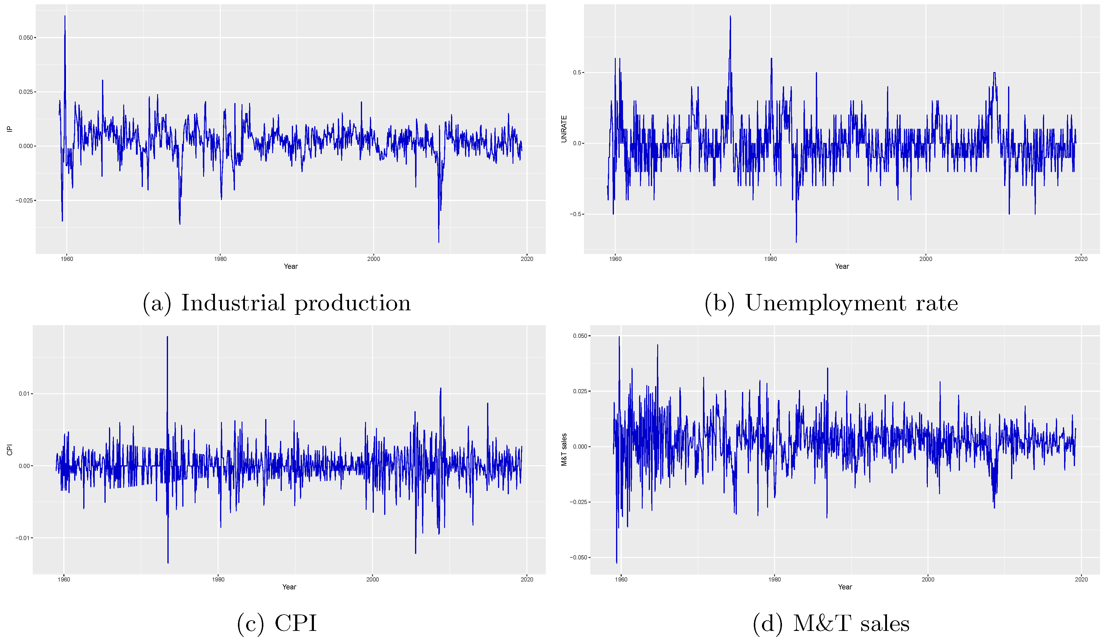
First, we consider the U.S. monthly macroeconomic data from January 1973 to June 2019. The data are from the FRED-MD database maintained by St. Louis Federal Reserve at https://research.stlouisfed.org/econ/mccracken/fred-databases/. We transform the time series to stationarity according to McCracken and Ng [9], and, after discarding some variables containing missing values, there are 125 macroeconomic time series. Among them, we focus on predicting (1) industrial production index, (2) unemployment rate, (3) CPI-All, and (4) Real manufacturing and trade industries sales (M&T sales). Time plots of these four target series after transformations are depicted in Figure 1.

For this data set, we consider

h = 1

and different combinations of q and r (the number of factors extracted). Since q lags of the predictors are used, there are

125 q

total predictors, which exceeds the sample size in each window. The last twenty years of data (240 time periods) are reserved for testing. In addition to the root mean squared forecasting errors, we also report the p-values of the Diebold-Mariano test [26,27] against the alternative hypothesis that the proposed GsP* procedure is more accurate.

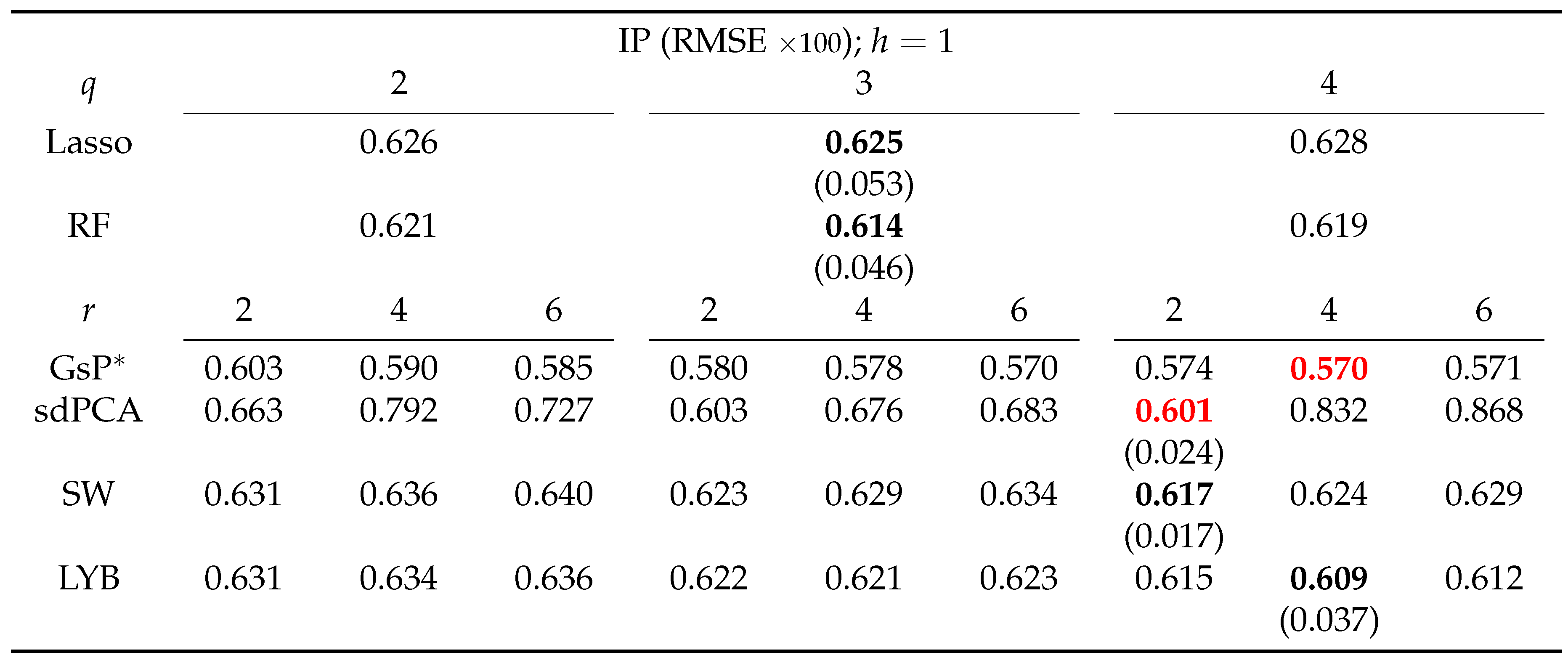
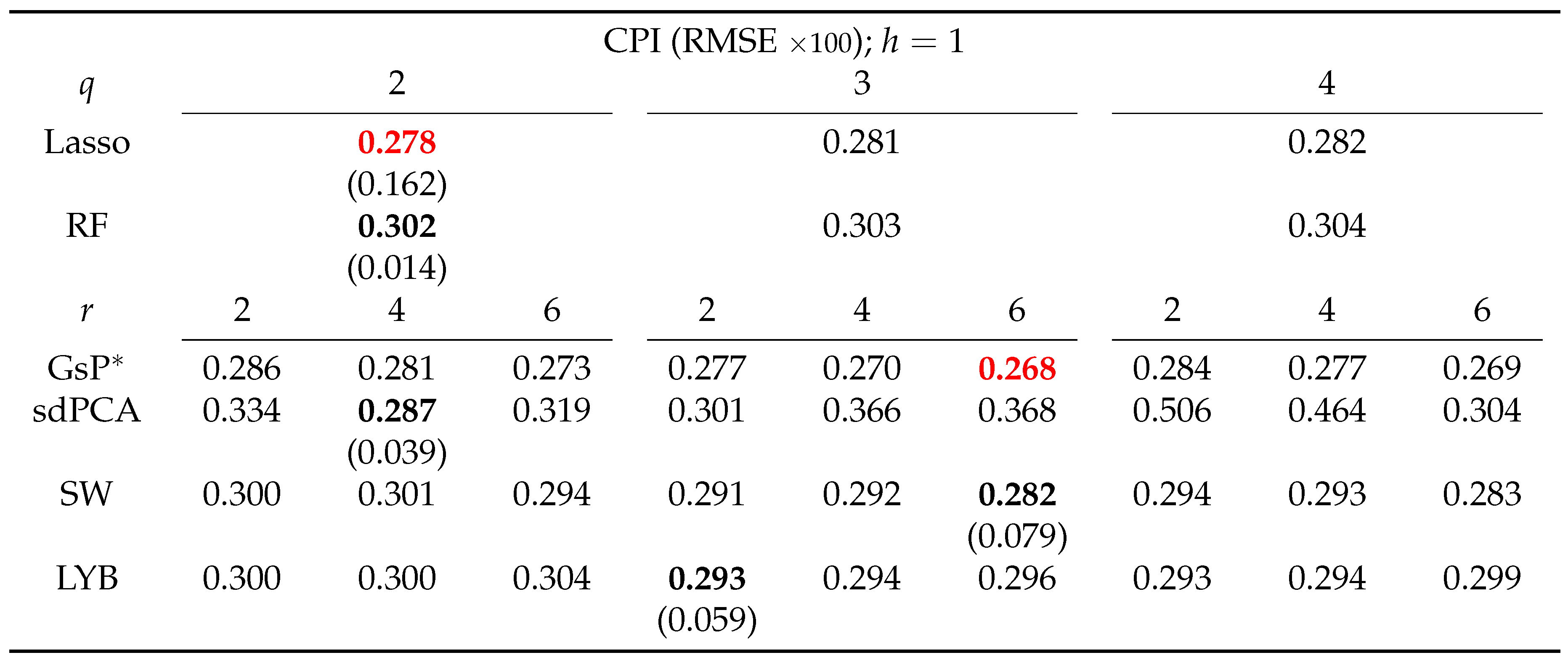
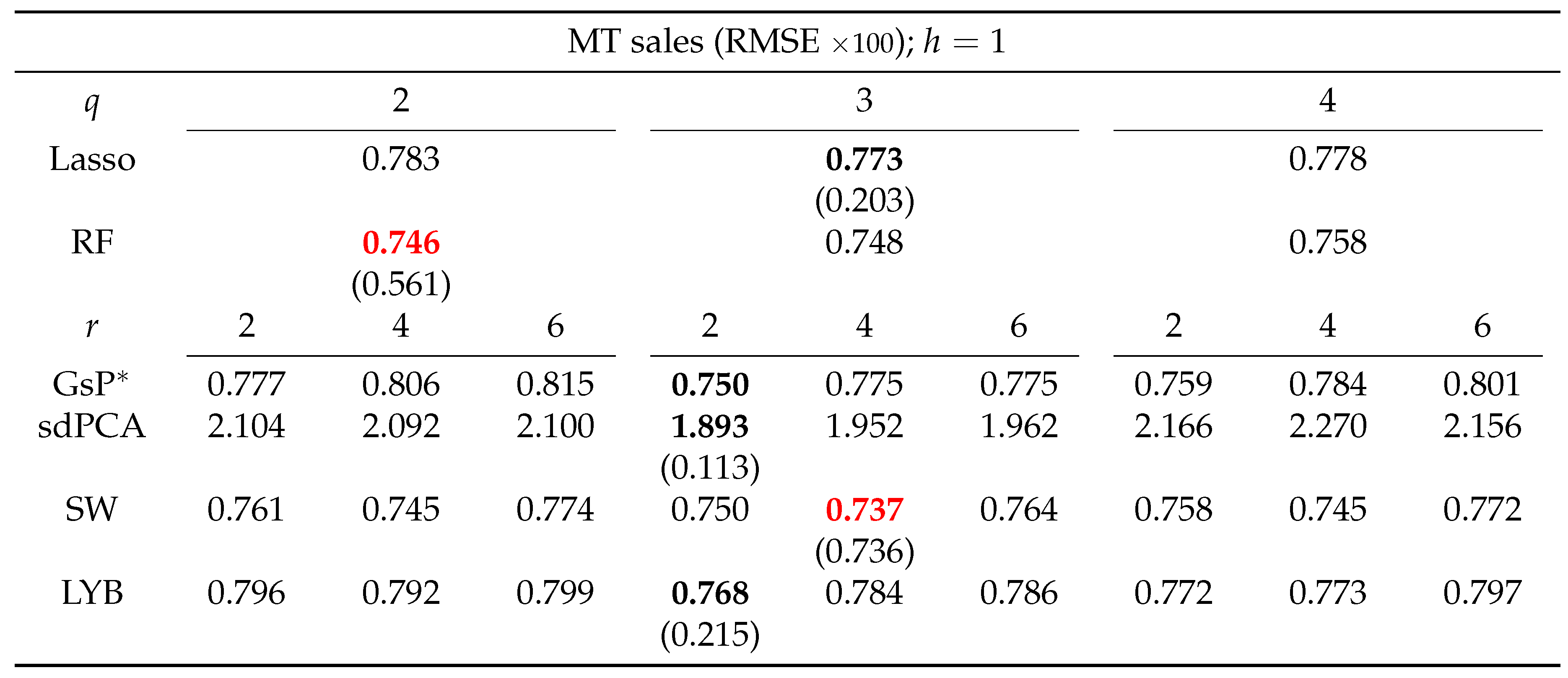
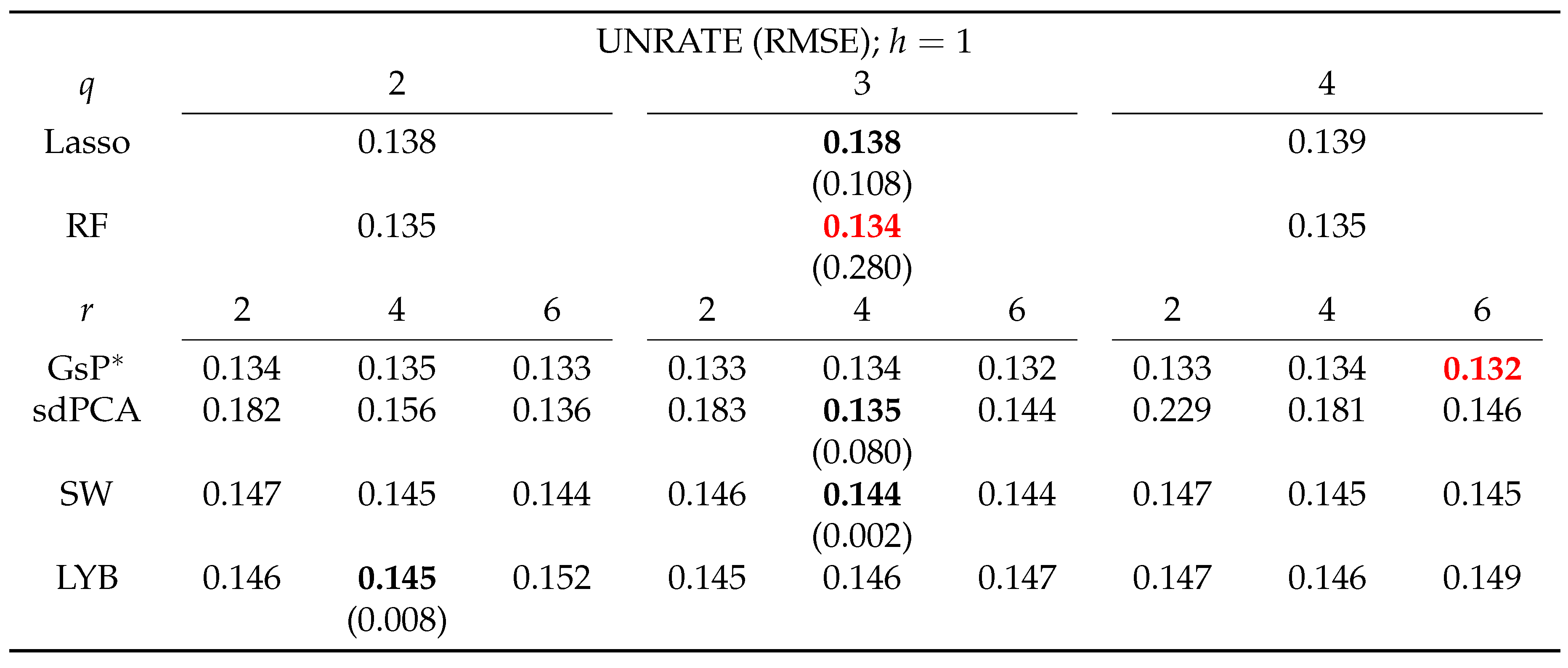
Table 4, Table 5, Table 6 and Table 7 present the results. The proposed GO-sdPCA achieved the lowest RMSFE for three of the targeted series: industrial production index, unemployment rate, and CPI. It notably outperformed the factor-based alternatives sdPCA, SW, and LYB with high confidence in forecasting these three series. In addition, no other methods demonstrated such consistent effectiveness across the targeted series.

6.2. Particulate Matters in Taiwan

We next consider the data of hourly PM_2.5 measurements in Taiwan during March of 2017. The data are sourced from the SLBDD package [28] in R. Each series in the data set represents measurements (in micrograms per cubic meters,

μ g / m^{3}

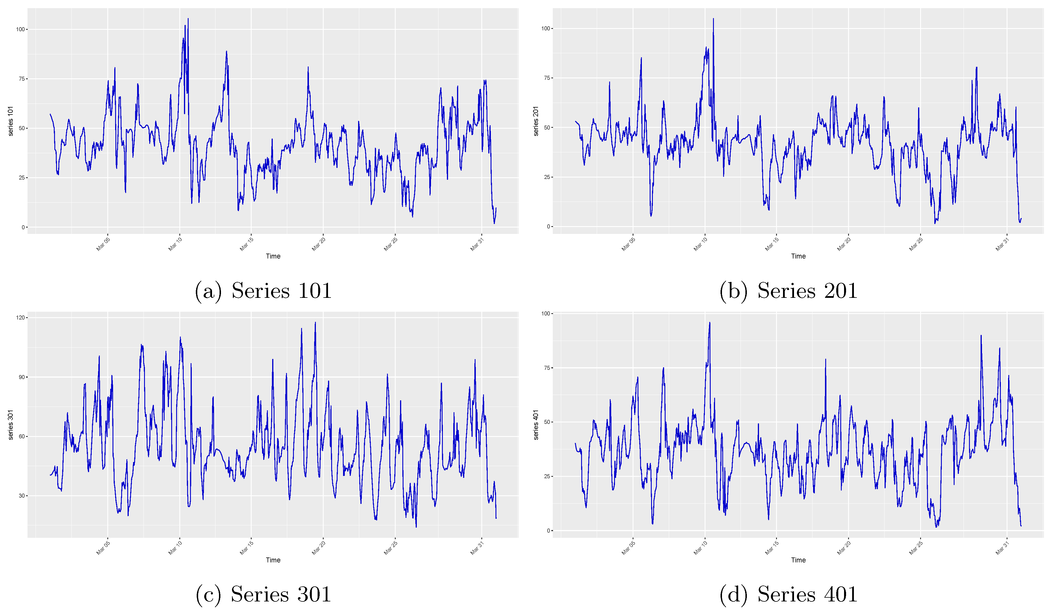
) taken by a novel device known as the AirBox. After an initial examination of these series, we remove series 29 and 70 because these series are near identically zero except at a few time points, offering no useful variations. Among the 516 series in the data set, we choose series 101, 201, 301, 401, as target series. Figure 2 depicts their time plots.

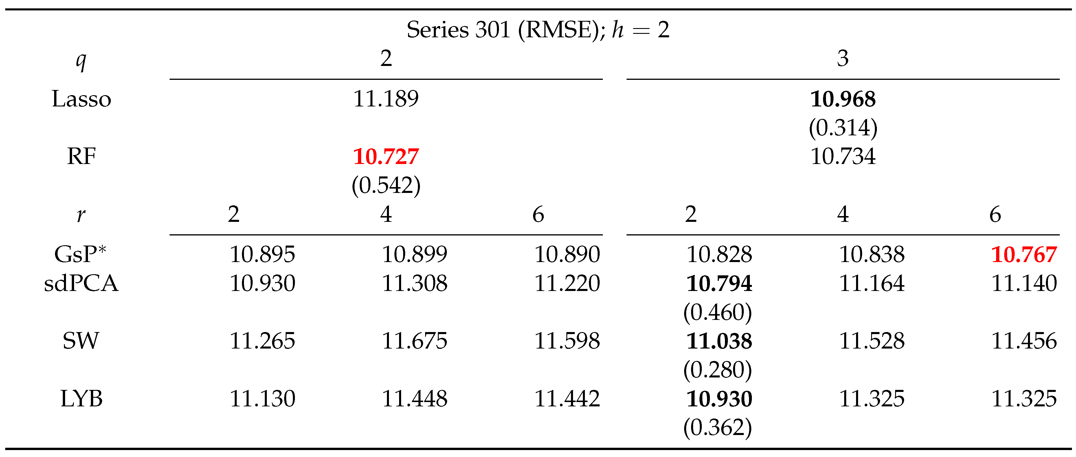
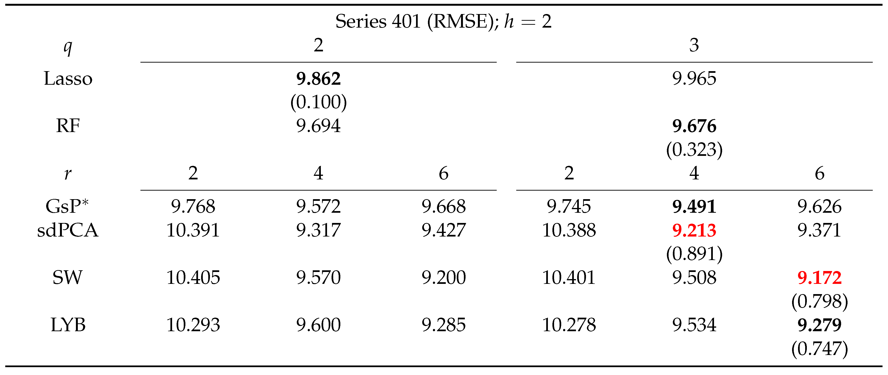
We consider both one-step-ahead (

h = 1

) and two-step-ahead (

h = 2

) forecasts, and employ

q \in {2, 3}

lags and

r \in {2, 4, 6}

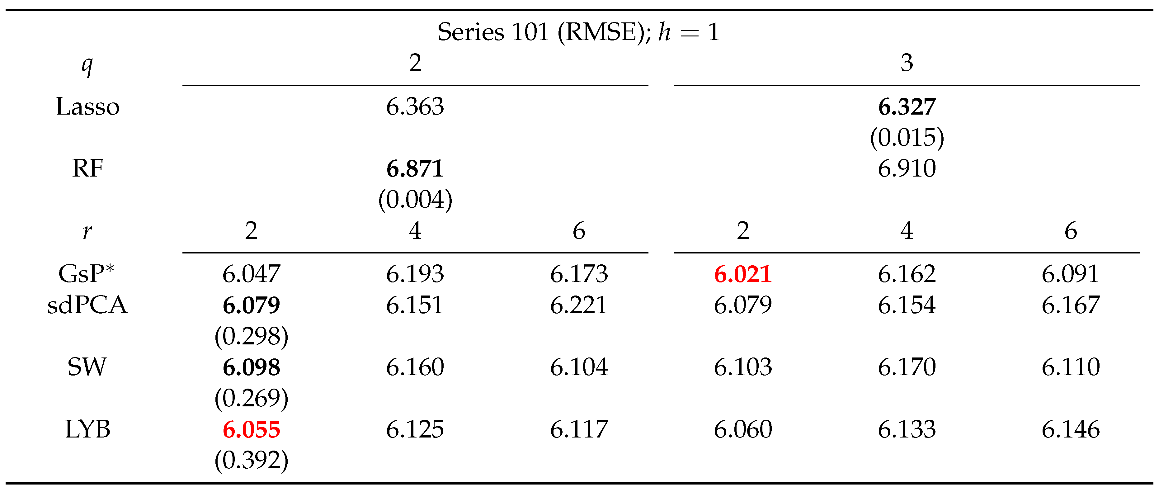
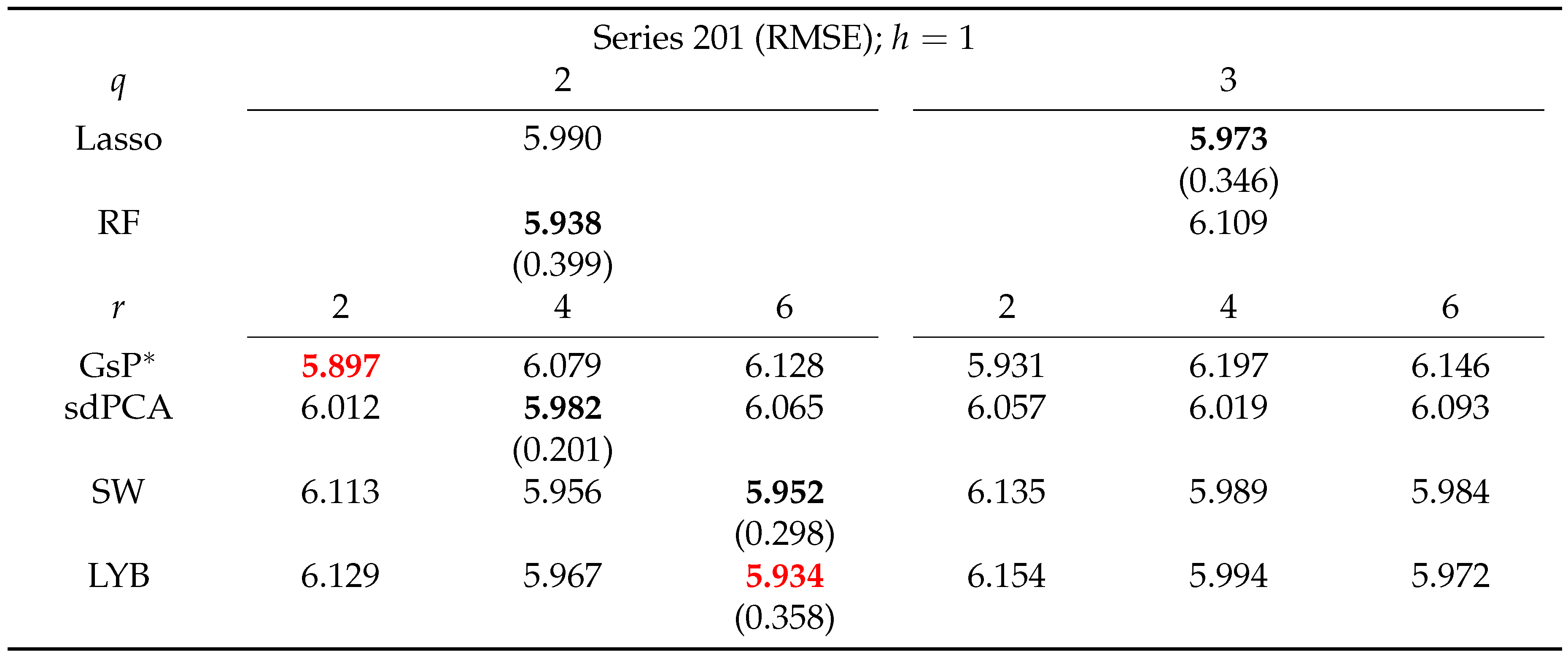
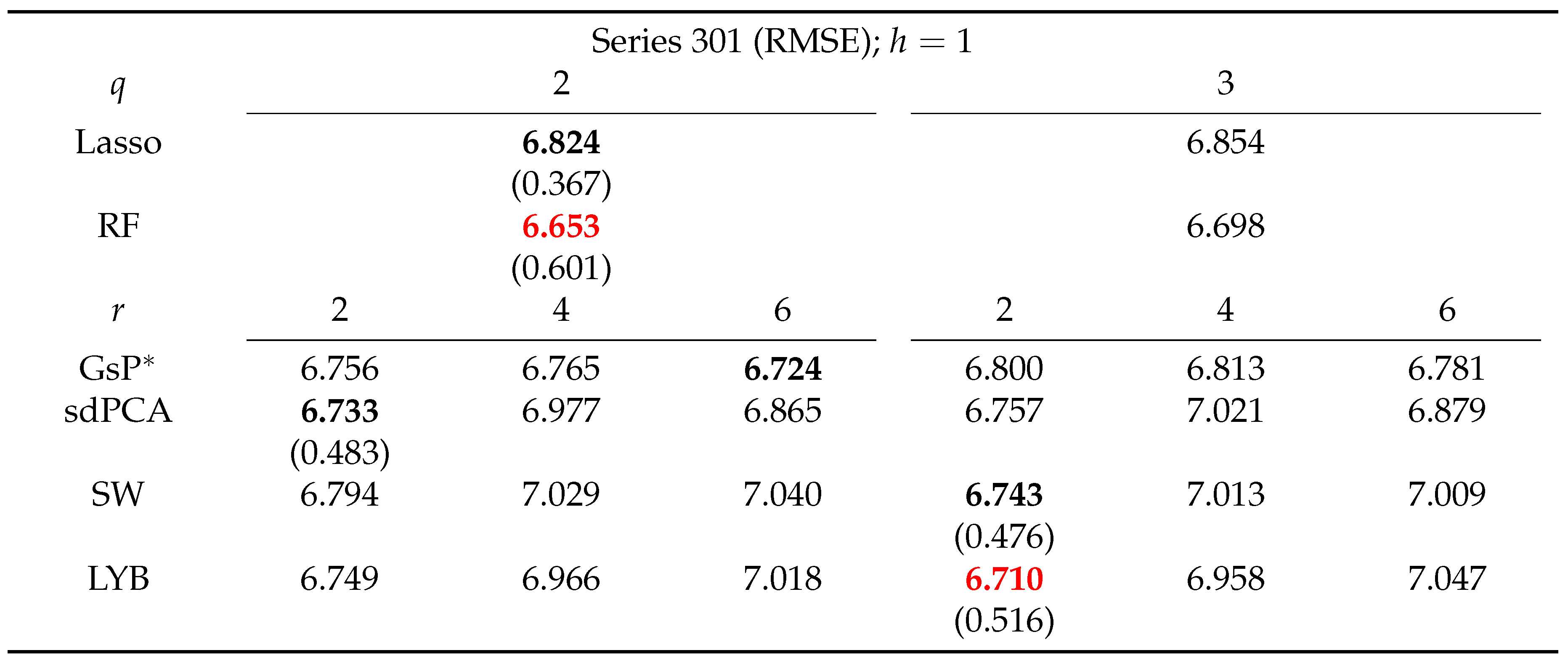
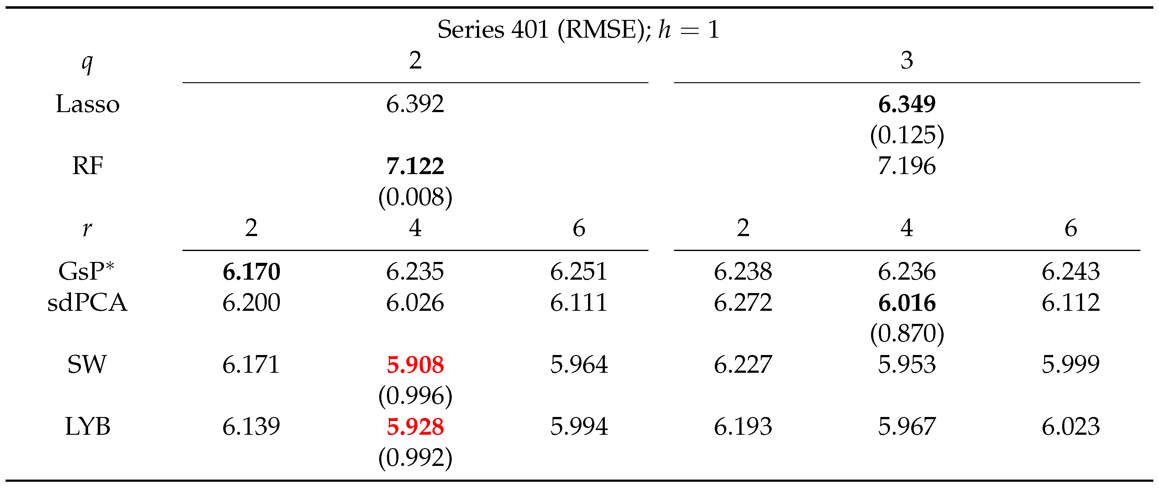
factors in forecasting. The last ten days of data (240 time periods) are reserved for out-of-sample testing. Table 8, Table 9, Table 10 and Table 11 present the results for

h = 1

. The proposed GO-sdPCA ranks as the most predictive method in terms of RMSFE for two of the four targeted series: Series 101 and 201. It outperforms the Lasso in forecasting all four targeted series. The performance of LYB is also noteworthy. It ranks among the best two methods for all four targeted series. The DM test, on the other hand, indicates the difference in forecasting accuracy is not statistically significant. Contrary to the case in the macroeconomic data, the proposed GsP* only outperformed the factor-based methods, including the sdPCA, with some weak confidence. 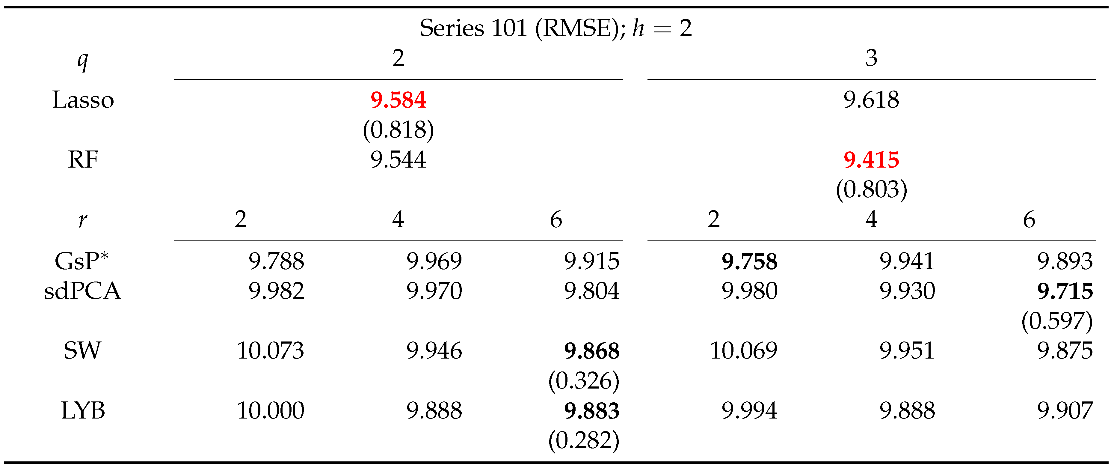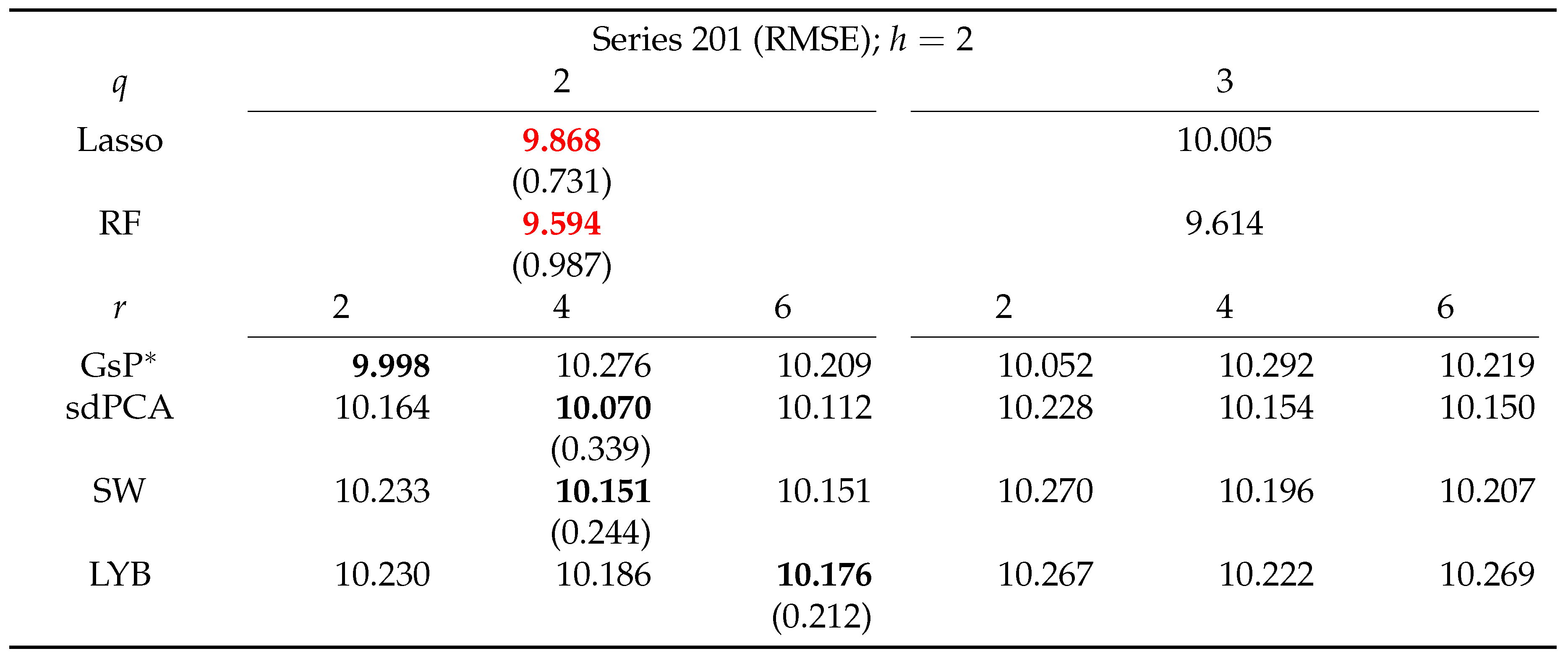For the two-step-ahead forecasts, for which the results are reported in Table 12, Table 13, Table 14 and Table 15, the performance of various methods is more entangled, with the RF consistently ranked among the top two methods for three of the four targeted series. With some weaker confidence, GsP* is the best performing factor-based method for two of the four targeted series. Again, the DM test fails to separate significantly various forecasting methods. We believe this result might be caused by the substantial uncertainty in the PM_2.5 measurements.

In sum, for

h = 1

, GsP* is effective in forecasting PM_2.5 data as well as the U.S. macroeconomic data. This implies the proposed procedure is able to capture highly predictive factors across various applications. On the other hand, for

h = 2

, the dynamic nature of the data may be much more involved. The performance of the proposed method becomes similar to those of the other forecasting methods.

7. Discussion and Concluding Remarks

In this work, we proposed a novel method for time series forecasting when many predictors are available. The rationale behind our method is to mine the possibly many (compared to the sample size) factor-relevant predictors while reducing the effect of the many irrelevant variables in the high-dimensional data. The results in the simulation studies and the empirical applications suggest that the proposed method is useful for improving upon both the factor-based methods and methods for sparse linear models such as the Lasso. Finally, we remark that the theoretical investigation of the peeling technique, a key ingredient in our method, would be an interesting topic for future research.

References

Peña, D.; Box, G.E. Identifying a simplifying structure in time series. Journal of the American statistical Association 1987, 82, 836–843. [Google Scholar] [CrossRef]
Stock, J.H.; Watson, M.W. Forecasting Using Principal Components From a Large Number of Predictors. Journal of the American Statistical Association 2002, 97, 1167–1179. [Google Scholar] [CrossRef]
Stock, J.H.; Watson, M.W. Macroeconomic Forecasting Using Diffusion Indexes. Journal of Business & Economic Statistics 2002, 20, 147–162. [Google Scholar]
Lam, C.; Yao, Q.; Bathia, N. Estimation of latent factors for high-dimensional time series. Biometrika 2011, 98, 901–918. [Google Scholar] [CrossRef]
Tsay, R.S. Multivariate time series analysis: with R and financial applications; John Wiley & Sons, 2013.
Bernanke, B.S.; Boivin, J. Monetary policy in a data-rich environment. Journal of Monetary Economics 2003, 50, 525–546. [Google Scholar] [CrossRef]
Bernanke, B.S.; Boivin, J.; Eliasz, P. Measuring the Effects of Monetary Policy: A Factor-Augmented Vector Autoregressive (FAVAR) Approach. The Quarterly Journal of Economics 2005, 120, 387–422. [Google Scholar]
Jurado, K.; Ludvigson, S.C.; Ng, S. Measuring Uncertainty. The American Economic Review 2015, 105, 1177–1216. [Google Scholar] [CrossRef]
McCracken, M.W.; Ng, S. FRED-MD: A Monthly Database for Macroeconomic Research. Journal of Business & Economic Statistics 2016, 34, 574–589. [Google Scholar]
Boivin, J.; Ng, S. Are more data always better for factor analysis? Journal of Econometrics 2006, 132, 169–194. [Google Scholar] [CrossRef]
Kim, H.H.; Swanson, N.R. Forecasting financial and macroeconomic variables using data reduction methods: New empirical evidence. Journal of Econometrics 2014, 178, 352–367. [Google Scholar] [CrossRef]
Huang, D.; Jiang, F.; Li, K.; Tong, G.; Zhou, G. Scaled PCA: A New Approach to Dimension Reduction. Management Science 2022, 68, 1678–1695. [Google Scholar] [CrossRef]
Gao, Z.; Tsay, R.S. Supervised Dynamic PCA: Linear Dynamic Forecasting with Many Predictors. Journal of the American Statistical Association, (accepted). 2024+. [Google Scholar] [CrossRef]
Chan, N.H.; Ing, C.K.; Li, Y.; Yau, C.Y. Threshold Estimation via Group Orthogonal Greedy Algorithm. Journal of Business & Economic Statistics 2017, 35, 334–345. [Google Scholar]
Ing, C.K. Model selection for high-dimensional linear regression with dependent observations. The Annals of Statistics 2020, 48, 1959–1980. [Google Scholar] [CrossRef]
Ing, C.K.; Lai, T.L. A STEPWISE REGRESSION METHOD AND CONSISTENT MODEL SELECTION FOR HIGH-DIMENSIONAL SPARSE LINEAR MODELS. Statistica Sinica 2011, 21, 1473–1513. [Google Scholar] [CrossRef]
Tibshirani, R. Regression Shrinkage and Selection via the Lasso. Journal of the Royal Statistical Society. Series B (Methodological) 1996, 58, 267–288. [Google Scholar] [CrossRef]
Breiman, L. Random Forests. Machine Learning 2001, 45, 5–32. [Google Scholar] [CrossRef]
Temlyakov, V. Greedy Approximation; Cambridge Monographs on Applied and Computational Mathematics, Cambridge University Press, 2011.
Barron, A.R.; Cohen, A.; Dahmen, W.; DeVore, R.A. Approximation and Learning by Greedy Algorithms. The Annals of Statistics 2008, 36, 64–94. [Google Scholar] [CrossRef]
James, G.; Witten, D.; Hastie, T.; Tibshirani, R. An Introduction to Statistical Learning with Appications in R, second ed.; Springer New York, NY, 2021.
Chi, C.M.; Vossler, P.; Fan, Y.; Lv, J. Asymptotic properties of high-dimensional random forests. The Annals of Statistics 2022, 50, 3415–3438. [Google Scholar] [CrossRef]
Saha, A.; Basu, S.; Datta, A. Random Forests for Spatially Dependent Data. Journal of the American Statistical Association 2023, 118, 665–683. [Google Scholar] [CrossRef]
Medeiros, M.C.; Mendes, E.F. ℓ₁-regularization of high-dimensional time-series models with non-Gaussian and heteroskedastic errors. Journal of Econometrics 2016, 191, 255–271. [Google Scholar] [CrossRef]
Liaw, A.; Wiener, M. Classification and Regression by randomForest. R News 2002, 2, 18–22. [Google Scholar]
Diebold, F.X.; Mariano, R.S. Comparing Predictive Accuracy. Journal of Business & Economic Statistics 1995, 13, 253–263. [Google Scholar]
Harvey, D.; Leybourne, S.; Newbold, P. Testing the equality of prediction mean squared errors. International Journal of Forecasting 1997, 13, 281–291. [Google Scholar] [CrossRef]
Caro, A.; Elias, A.; Peña, D.; Tsay, R.S. SLBDD: Statistical Learning for Big Dependent Data, 2022. R package version 0.0.4.

Figure 1. Time plots of the (transformed) macroeconomic time series of interest.

Figure 2. Time plots of the four targeted hourly PM_2.5 measurements on Taiwan in March 2017.

Table 1. Root mean squared forecast error of various competing methods. The data are generated from DGP 1 and the results are averaged over 500 Monte Carlo simulations. n and p stand for the sample size and number of observed predictors.

r_{DGP}

is defined in DGP 1, and r is the number of factors extracted using various methods.

r_{DGP}

is defined in DGP 1, and r is the number of factors extracted using various methods.

	GsP*	GsP	sdPCA	SW	LYB	Lasso	RF
$(r_{DGP}, s)$	$(n, p, r) = (200, 1000, 10)$
(5, 50)	1.894	2.443	1.993	2.657	2.136	2.207	2.860
(10, 100)	2.406	3.299	2.488	3.288	2.909	2.831	4.353
(15, 150)	3.315	3.908	3.584	5.368	5.201	3.537	5.776
$(n, p, r) = (400, 2000, 30)$
(10, 100)	2.391	2.947	2.590	3.482	2.077	2.544	4.428
(20, 200)	3.020	4.355	3.242	4.626	3.657	3.679	6.604
(30, 300)	3.818	5.581	4.155	5.666	4.651	4.450	8.253

Table 2. Root mean squared forecast error of the competing methods, divided by 1000. Data are generated from DGP 2 and the results are averaged over 500 Monte Carlo simulations. n and p stand for the sample size and number of observed predictors.

r_{DGP}

is defined in DGP 2, r is the number of factors extracted using various methods, and s is a sparsity parameter.

r_{DGP}

is defined in DGP 2, r is the number of factors extracted using various methods, and s is a sparsity parameter.

	GsP*	GsP	sdPCA	SW	LYB	Lasso	RF
$(r_{DGP}, s)$	$(n, p, r) = (200, 1000, 10)$
(5, 50)	0.857	0.883	0.695	1.017	0.966	0.870	2.017
(10, 100)	2.833	3.137	2.834	3.436	3.436	3.802	6.971
(15, 150)	6.559	7.068	6.379	7.801	7.761	9.532	16.264
$(n, p, r) = (400, 2000, 30)$
(10, 100)	4.091	4.547	2.259	5.224	4.917	5.118	8.977
(20, 200)	15.891	17.357	8.411	20.012	19.411	20.961	35.132
(30, 300)	34.557	37.956	34.543	42.904	42.905	50.996	70.180

Table 3. Root mean squared forecast error of various competing methods. Data are generated from DGP 3 and the results are averaged over 500 Monte Carlo simulations. n and p stand for the sample size and number of observed predictors.

r_{DGP}

is defined in DGP 3, and r is the number of factors extracted using various methods.

r_{DGP}

is defined in DGP 3, and r is the number of factors extracted using various methods.

	GsP*	GsP	sdPCA	SW	LYB	Lasso	RF
$(r_{DGP}, s)$	$(n, p, r) = (200, 1000, 10)$
(5, 50)	12.255	12.166	12.347	12.565	12.469	7.537	12.813
(10, 100)	17.818	18.857	17.608	17.371	17.701	16.670	18.427
(15, 150)	23.142	24.417	23.041	21.777	22.027	21.125	22.660
$(n, p, r) = (400, 1000, 30)$
(10, 100)	16.523	17.540	17.767	18.647	18.968	14.833	18.602
(20, 200)	27.266	29.110	26.063	25.291	25.717	25.953	26.503
(30, 300)	33.763	35.635	32.438	31.672	31.827	31.340	32.427

Table 4. Root mean squared forecast errors

\times 100

for predicting industrial production index. The lowest RMSFE achieved by each method is in boldface. Among these boldfaced values, the lowest two values are marked in red. q denotes the number of lags used in estimation and r is the number of factors extracted. GsP* denotes the proposed GO-sdPCA. The figures in the parentheses are the p-values of the Diebold-Mariano test of whether GsP* is more accurate.

Table 4. Root mean squared forecast errors

\times 100

Table 5. Root mean squared forecast errors for predicting unemployment rate. The lowest RMSFE achieved by each method is in boldface. Among these boldfaced values, the lowest two values are marked in red. q denotes the number of lags used in estimation and r is the number of factors extracted. GsP* denotes the proposed GO-sdPCA. The figures in the parentheses are the p-values of the Diebold-Mariano test of whether GsP* is more accurate.

Table 6. Root mean squared forecast errors

\times 100

for predicting CPI. The lowest RMSFE achieved by each method is in boldface. Among these boldfaced values, the lowest two values are marked in red. q denotes the number of lags used in estimation and r is the number of factors extracted. GsP* denotes the proposed GO-sdPCA. The figures in the parentheses are the p-values of the Diebold-Mariano test of whether GsP* is more accurate.

Table 6. Root mean squared forecast errors

\times 100

Table 7. Root mean squared forecast errors

\times 100

for predicting MT sales. The lowest RMSFE achieved by each method is in boldface. Among these boldfaced values, the lowest two values are marked in red. q denotes the number of lags used in estimation and r is the number of factors extracted. GsP* denotes the proposed GO-sdPCA. The figures in the parentheses are the p-values of the Diebold-Mariano test of whether GsP* is more accurate.

Table 7. Root mean squared forecast errors

\times 100

Table 8. Root mean squared forecast errors for predicting series 101 in Taiwan PM_2.5 data. The forecast horizon h is 1. The lowest RMSFE achieved by each method is in boldface. Among these boldfaced values, the lowest two values are marked in red. q denotes the number of lags used in estimation and r is the number of factors extracted. GsP* denotes the proposed GO-sdPCA. The figures in the parentheses are the p-values of the Diebold-Mariano test of whether GsP* is more accurate.

Table 9. Root mean squared forecast errors for predicting series 201 in Taiwan PM_2.5 data. The forecast horizon h is 1. The lowest RMSFE achieved by each method is in boldface. Among these boldfaced values, the lowest two values are marked in red. q denotes the number of lags used in estimation and r is the number of factors extracted. GsP* denotes the proposed GO-sdPCA. The figures in the parentheses are the p-values of the Diebold-Mariano test of whether GsP* is more accurate.

Table 10. Root mean squared forecast errors for predicting series 301 in Taiwan PM_2.5 data. The forecast horizon h is 1. The lowest RMSFE achieved by each method is in boldface. Among these boldfaced values, the lowest two values are marked in red. q denotes the number of lags used in estimation and r is the number of factors extracted. GsP* denotes the proposed GO-sdPCA. The figures in the parentheses are the p-values of the Diebold-Mariano test of whether GsP* is more accurate.

Table 11. Root mean squared forecast errors for predicting series 401 in Taiwan PM_2.5 data. The forecast horizon h is 1. The lowest RMSFE achieved by each method is in boldface. Among these boldfaced values, the lowest two values are marked in red. q denotes the number of lags used in estimation and r is the number of factors extracted. GsP* denotes the proposed GO-sdPCA. The figures in the parentheses are the p-values of the Diebold-Mariano test of whether GsP* is more accurate.

Table 12. Root mean squared forecast errors for predicting series 101 in Taiwan PM_2.5 data. The forecast horizon h is 2. The lowest RMSFE achieved by each method is in boldface. Among these boldfaced values, the lowest two values are marked in red. q denotes the number of lags used in estimation and r is the number of factors extracted. GsP* denotes the proposed GO-sdPCA. The figures in the parentheses are the p-values of the Diebold-Mariano test of whether GsP* is more accurate.

Table 13. Root mean squared forecast errors for predicting series 201 in Taiwan PM_2.5 data. The forecast horizon h is 2. The lowest RMSFE achieved by each method is in boldface. Among these boldfaced values, the lowest two values are marked in red. q denotes the number of lags used in estimation and r is the number of factors extracted. GsP* denotes the proposed GO-sdPCA. The figures in the parentheses are the p-values of the Diebold-Mariano test of whether GsP* is more accurate.

Table 14. Root mean squared forecast errors for predicting series 301 in Taiwan PM_2.5 data. The forecast horizon h is 2. The lowest RMSFE achieved by each method is in boldface. Among these boldfaced values, the lowest two values are marked in red. q denotes the number of lags used in estimation and r is the number of factors extracted. GsP* denotes the proposed GO-sdPCA. The figures in the parentheses are the p-values of the Diebold-Mariano test of whether GsP* is more accurate.

Table 15. Root mean squared forecast errors for predicting series 401 in Taiwan PM_2.5 data. The forecast horizon h is 2. The lowest RMSFE achieved by each method is in boldface. Among these boldfaced values, the lowest two values are marked in red. q denotes the number of lags used in estimation and r is the number of factors extracted. GsP* denotes the proposed GO-sdPCA. The figures in the parentheses are the p-values of the Diebold-Mariano test of whether GsP* is more accurate.

Disclaimer/Publisher’s Note: The statements, opinions and data contained in all publications are solely those of the individual author(s) and contributor(s) and not of MDPI and/or the editor(s). MDPI and/or the editor(s) disclaim responsibility for any injury to people or property resulting from any ideas, methods, instructions or products referred to in the content.

© 2024 by the authors. Licensee MDPI, Basel, Switzerland. This article is an open access article distributed under the terms and conditions of the Creative Commons Attribution (CC BY) license (http://creativecommons.org/licenses/by/4.0/).

Copyright: This open access article is published under a Creative Commons CC BY 4.0 license, which permit the free download, distribution, and reuse, provided that the author and preprint are cited in any reuse.

MDPI Initiatives

Important Links

Choose an area of interest and we will send you notifications of new preprints at your preferred frequency.

Disclaimer

Time Series Forecasting with Many Predictors

Abstract

1. Introduction

2. Orthogonal Greedy Algorithm

3. Supervised Dynamic PCA

4. The Proposed GO-sdPCA

5. Simulation Studies

5.1. Simulation Designs and Results

6. Empirical Examples

6.1. U.S. Macroeconomic Data

6.2. Particulate Matters in Taiwan

7. Discussion and Concluding Remarks

References

MDPI Initiatives

Important Links

Subscribe