Erroneous Applications of Fractional Calculus: The Catenary as a Prototype

Preprint

Article

Erroneous Applications of Fractional Calculus: The Catenary as a Prototype

Altmetrics

Downloads

Views

Comments

A peer-reviewed article of this preprint also exists.

Gerardo Becerra-Guzmán,

José Villa-Morales^*

Gerardo Becerra-Guzmán,

José Villa-Morales^*

This version is not peer-reviewed

Submitted:

19 June 2024

Posted:

24 June 2024

You are already at the latest version

Alerts

Abstract

In this work, we study the equation of the catenary curve in the context of the Caputo derivative. We solve this equation and compare the solution with real physical models. From the experiments, we find that the best approximation is achieved in the classical case. Therefore, introducing a fractional parameter arbitrarily can be detrimental. However, we observe that when adding a certain weight to the chain, fractional calculus produces better results than classical calculus for modeling the minimum height.

Keywords:

Subject: Computer Science and Mathematics - Applied Mathematics

MSC: 34A08; 34A34; 34A06; 35R11

1. Introduction and Statement of the Results

The catenary curve, that elegant and resilient shape describing the configuration of a hanging chain, has left an indelible mark on the modern world. In the field of civil engineering, the catenary has played a fundamental role in the design of iconic structures, such as the Sagrada Familia church in Barcelona, Spain. Furthermore, its ability to evenly distribute loads along its curve makes it an ideal solution for bridges, arches, and other structures that must bear heavy weights.

The influence of the catenary extends far beyond civil engineering. In dentistry, its shape describes the natural curvature of healthy dental arches, providing a basis for understanding oral anatomy and designing dental prostheses. In the oil industry, the catenary is used to optimize well drilling, ensuring an efficient and safe trajectory. Even in the medical field, the catenary is employed to measure breast curvature in cancer diagnosis, providing crucial information for the detection and treatment of this disease (see [1,2], or the references mentioned therein).

The fascination with the catenary dates back to the time of Galileo Galilei, who compared the shape of a hanging chain to a parabola. However, it was Joachim Jungius who demonstrated that hanging chains have a distinct shape, laying the groundwork for a deeper study of this curve. In 1691, the catenary was formally defined and named, opening the doors to countless applications (see [3]).

The catenary curve, with its rich history and diverse applications, continues to inspire researchers and professionals in various fields. Its still untapped potential opens up new possibilities for designing stronger, more efficient, and more aesthetic structures, as well as for better understanding natural and complex phenomena. The catenary will undoubtedly remain a cornerstone of the modern world and a symbol of human creativity and ingenuity.

In this context, it is natural to consider the differential equation modeling the catenary curve in the fractional context, as we will do next to explore a new facet of the catenary. It should be noted that the equation modeling the catenary curve has already been studied in [4] using the Caputo-Fabrizio derivative. Here we will use the fractional derivative in the sense of Caputo. The Caputo-Fabrizio derivative involves a non-singular kernel and when modeling it often yields different results from the Caputo derivative (see [5]).

Nowadays, it unfortunately happens all too often that a classical differential equation is considered, and instead of the integer-order derivative operator, it is replaced by a fractional derivative operator. In the vast majority of these cases, it is tacitly assumed that the fractional dynamics improve the model obtained using classical differential calculus. Under this premise, that is, assuming there is an improvement using fractional calculus, various authors engage in a series of theoretical developments or numerical manipulations that later make no sense (see [6]).

To illustrate this point, we have chosen the catenary curve because, as we mentioned before, it is an important phenomenon and relatively easy to reproduce. Using a hanging chain and a scanner, one can obtain the shape of the catenary curve (see Section 3). Furthermore, the associated differential equation is a second-order nonlinear differential equation (see (2.2)-(2.3)). By replacing the integer-order derivative with the fractional-order derivative (see (2.2) and (4.1)), a fractional differential equation is obtained (see (4.4)). This equation is solved, and the key point here is that the fractional parameters do not model the physical curve of the hanging chain. In other words, it is generally incorrect to think that the fractional model improves the classical model. In some cases, such as in the study of control systems, nonlinear and nonlocal models are often modeled by nonlinear fractional differential equations (see [6]). In our case, we see that this is not the case; indeed, the modeling of the catenary is a nonlinear model, and any (local) perturbation of the chain affects the chain globally.

On the other hand, when a certain weight is applied to the center of the chain, relatively minor compared to the total weight of the chain, it is observed that there are fractional indices that better model the deformed curve than the classical case. This is consistent with what is known (that it is a nonlocal phenomenon) and opens a possible opportunity for fractional calculus to model this phenomenon, at least improving the classical case. In this case, as we mentioned, by modifying the weight of the chain at its center, the overall structure of the curve is altered; changes are not limited to a neighborhood of the center of the catenary. Since modeling the catenary curve with weight classically is a complicated problem (see [8] or [9]) and using fractional calculus we achieve it with little effort, we can say that for modeling this phenomenon, fractional calculus proves to be useful.

In summary, the fractional index should not be introduced into a differential equation without real evidence that it improves the model (see [6]). At best, the fractional analytical model represents a perturbation of the classical model. This observation should not be taken lightly, as there is a wide variety of fractional derivatives, and theoretical aspects are sometimes studied without any basis other than the aesthetic aspect of mathematics (see [11] and [10]).

The article is organized as follows. In Section 2, we recall the derivation of the classical catenary, which serves to introduce some concepts and propose the relevant modifications in the fractional case. In Section 3, we define some concepts of fractional calculus and state some basic properties. In Section 4, we present the fractional differential equation in the sense of Caputo and solve it. In Section 5, we describe the physical experiment and present some images of catenaries. Finally, in Section 6, we present some conclusions.

2. Classical Catenary Curve

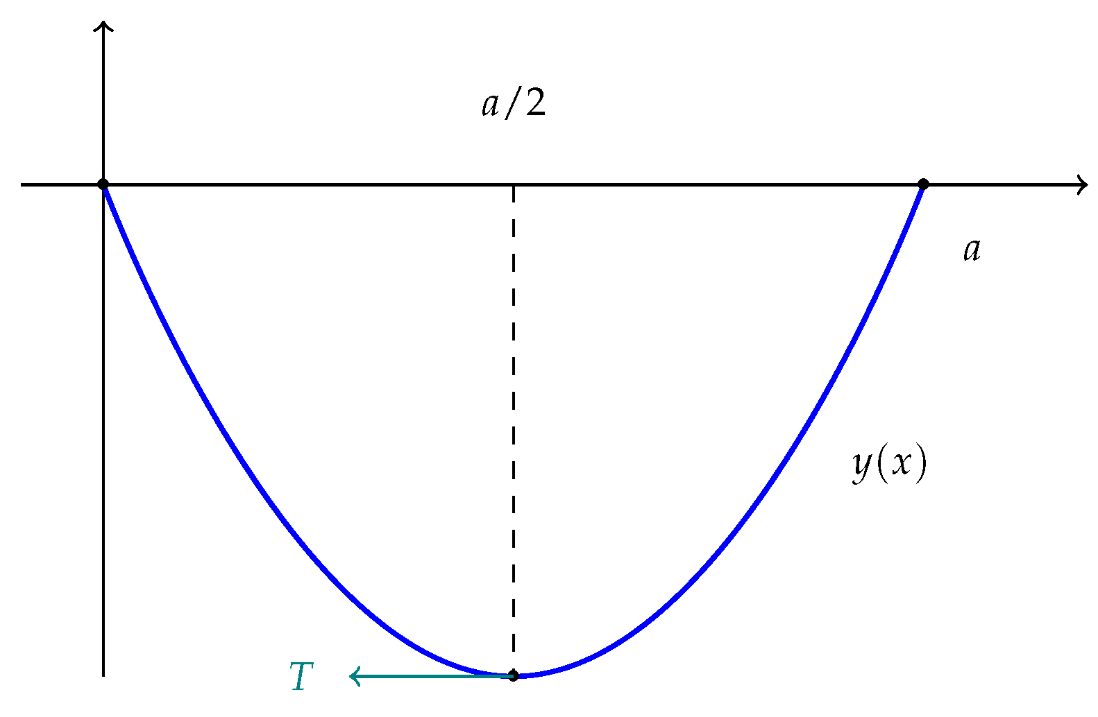
In this section, we will briefly review the classical derivation of the catenary curve. Consider a homogeneous rope or string with linear density

ρ

and a length greater than a, where a is a fixed positive number. Let T represent the tension at the midpoint

a / 2

. With this information, we can create a diagram similar to the one shown in Figure 1.

Carrying out an analysis of the forces (see, for example, [7]), we arrive at the following equation

\frac{1}{c} \int_{a / 2}^{x} \sqrt{1 + {(u (t))}^{2}} d t = u (x), x \in (0, a),

(1)

where

u (x) = y^{'} (x),

(2)

c = T / (g ρ)

, and g is the gravitational constant. Taking derivatives in (1), we deduce the second-order nonlinear differential equation

\frac{1}{c} \sqrt{1 + {(u (x))}^{2}} = u^{'} (x),

(3)

with initial condition

u (a / 2) = y^{'} (a / 2) = 0 .

(4)

The general solution of (3) has the form

u (x) = sinh (\frac{1}{c} x + c_{0}), x \in [0, a],

(5)

where

c_{0}

is a constant. Using the initial conditions (4), we obtain

c_{0} = - \frac{a}{2 c} .

(6)

Now, from (2) and using that

y (0) = 0

we get the classical catenary curve

y (x) = c \{cosh (\frac{x}{c} - \frac{a}{2 c}) - cosh (\frac{a}{2 c})\}, x \in [0, a] .

(7)

The minimum of the curve will be

y (\frac{a}{2}) = c \{1 - cosh (\frac{a}{2 c})\}, x \in [0, a] .

3. Some Preliminaries on Fractional Calculus

To introduce the fractional model of the catenary curve, it is helpful to revisit some key concepts of fractional calculus. Numerous excellent texts are available on this subject; for our purposes, we will adopt the notation and refer to the results presented in [13] and [12].

Definition 1.

Let

f : [a, b] \to R

be a continuous function. The left Riemann-Liouville integral,

I_{a +}^{α} f

, of f of order

α \in R

, is defined as

(I_{a +}^{α} f) (x) = \frac{1}{Γ (α)} \int_{a}^{x} \frac{f (t)}{{(x - t)}^{1 - α}} d t, x \in (a, b) .

Now let us suppose that

α > 0

and set

n : = [α] + 1

, where

[\cdot]

is the largest integer less than or equal to α. If

f^{(n)}

exists and is continuous, then the fractional derivative of Caputo, by the left, ^C

D_{a +}^{α} f

, is defined as

(^{C} D_{a +}^{α} f) (x) = (I_{a +}^{n - α} f^{(n)}) (x) = \frac{1}{Γ (n - α)} \int_{a}^{x} \frac{f^{(n)} (t)}{{(x - t)}^{1 + α - n}} d t, x \in (a, b) .

In the above definition,

Γ (α)

, with

α > 0

, represents the usual gamma function. Since we will not be utilizing any other fractional derivative, we will omit the C in the definition of a Caputo derivative, denoting it simply as

D^{α} f

Proposition 1.

Let

α > 0

and

n : = [α] + 1

. If f has has continuous derivatives up to order

n - 1

and

f^{(n)}

is absolutely continuous, then

(I_{a +}^{α} D_{a +}^{α} f) (x) = f (x) - \sum_{k = 0}^{n - 1} \frac{f^{(k)} (a)}{k!} {(x - a)}^{k} .

Proof.

See Lemma 2.22 in [12]. □

The linearity of the classical integral implies the linearity of the fractional integral. Furthermore, we have the following result.

Proposition 2.

Let

α \geq 0

and

β > 0

, then

(I_{a +}^{α} {(t - a)}^{β - 1}) (x) = \frac{Γ (β)}{Γ (β + α)} {(x - a)}^{β + α - 1} .

Proof.

See formulas (2.1.16) of [12]. □

4. Fractional Catenary Curve

Let

α \in (R_{+} ∖ N)

and

n : = [α] + 1

. A common method to extend the classical model to the fractional context involves introducing the fractional derivative operator into expression (2), thereby replacing the classical derivative with the fractional one, see [6] or [4],

u = D_{\frac{a}{2} +}^{α} y .

(8)

On the other hand, physical conditions require that the resulting curve be symmetric. Keeping this in mind, we consider the following equation (see equation (1)):

\begin{matrix} \frac{1}{c} \int_{a / 2}^{x} \sqrt{1 + {(u (t))}^{2}} d t = u (x), \frac{a}{2} < x < a . \end{matrix}

(9)

If we take the derivative, we obtain the fractional differential equation,

\frac{1}{c} \sqrt{1 + {(D_{\frac{a}{2} +}^{α} y (x))}^{2}} = D_{\frac{a}{2} +}^{1 + α} y (x),

(10)

with boundary conditions

y (a) = 0, y^{'} (\frac{a}{2}) = 0, \dots, y^{(n)} (\frac{a}{2}) = 0 .

(11)

The equation (9) is the same as equation (1), thus the solution is given by (5),

\begin{matrix} u (x) = sinh (\frac{1}{c} x + c_{1}), \frac{a}{2} < x < a, \end{matrix}

(12)

for some constant

c_{1}

. From the Proposition 1 we get

\begin{matrix} y (x) - \sum_{k = 0}^{n} \frac{y_{+}^{(k)} (\frac{a}{2})}{k!} {(x - \frac{a}{2})}^{k} = (I_{\frac{a}{2} +}^{α} D_{\frac{a}{2} +}^{α} y) (x) = I_{\frac{a}{2} +}^{α} u (x) . \end{matrix}

(13)

On the other hand, using (12) and the linearity of fractional integral we obtain

\begin{matrix} I_{\frac{a}{2} +}^{α} u (x) = \sum_{k = 0}^{\infty} \frac{1}{(2 k + 1)!} I_{\frac{a}{2} +}^{α} {(\frac{1}{c} x + c_{1})}^{2 k + 1} . \end{matrix}

(14)

Since

\begin{matrix} {(\frac{1}{c} x + c_{1})}^{2 k + 1} & = & {(\frac{1}{c})}^{2 k + 1} \sum_{j = 0}^{2 k + 1} (\binom{2 k + 1}{j}) {(\frac{a}{2} + c \cdot c_{1})}^{2 k + 1 - j} {(x - \frac{a}{2})}^{j}, \end{matrix}

then Proposition 2 and (11) yield

\begin{matrix} y (x) & = & \sum_{k = 0}^{n} \frac{y^{(k)} (\frac{a}{2})}{k!} {(x - \frac{a}{2})}^{k} + I_{\frac{a}{2} +}^{α} u (x) \\ = & y (\frac{a}{2}) + \sum_{k = 0}^{\infty} {(\frac{1}{c})}^{2 k + 1} \sum_{j = 0}^{2 k + 1} \frac{1}{(2 k + 1 - j)! Γ (j + 1 + α)} {(\frac{a}{2} + c \cdot c_{1})}^{2 k + 1 - j} {(x - \frac{a}{2})}^{j + α} . \end{matrix}

By hypothesis, the n-th derivative of y exists at

a / 2

. Since

α - n < 0

, then

\frac{a}{2} + c \cdot c_{1} = 0,

otherwise,

y^{(n)} (a / 2)

would not exist. This particular value of

c_{0}

corresponds to the classical case, as depicted in (6). Therefore, (11) suggests

\begin{matrix} y (x) = \sum_{k = 0}^{\infty} {(\frac{1}{c})}^{2 k + 1} \frac{1}{Γ (2 k + 2 + α)} [{(x - \frac{a}{2})}^{2 k + 1 + α} - {(\frac{a}{2})}^{2 k + 1 + α}], \frac{a}{2} \leq x \leq a . \end{matrix}

The fractional catenary curve

y_{α}

is given by

y_{α} (x) = \{\begin{matrix} y (a - x), & 0 \leq x \leq \frac{a}{2}, \\ y (x), & \frac{a}{2} \leq x \leq a . \end{matrix}

(15)

When

α = 1

, employing the Taylor series of the hyperbolic cosine yields the classical catenary (7). In the fractional scenario, the minimum is given by

y_{α} (\frac{a}{2}) = - c^{α} \sum_{k = 0}^{\infty} \frac{1}{Γ (2 k + 2 + α)} {(\frac{a}{2 c})}^{2 k + 1 + α} .

(16)

5. Physical Experiments

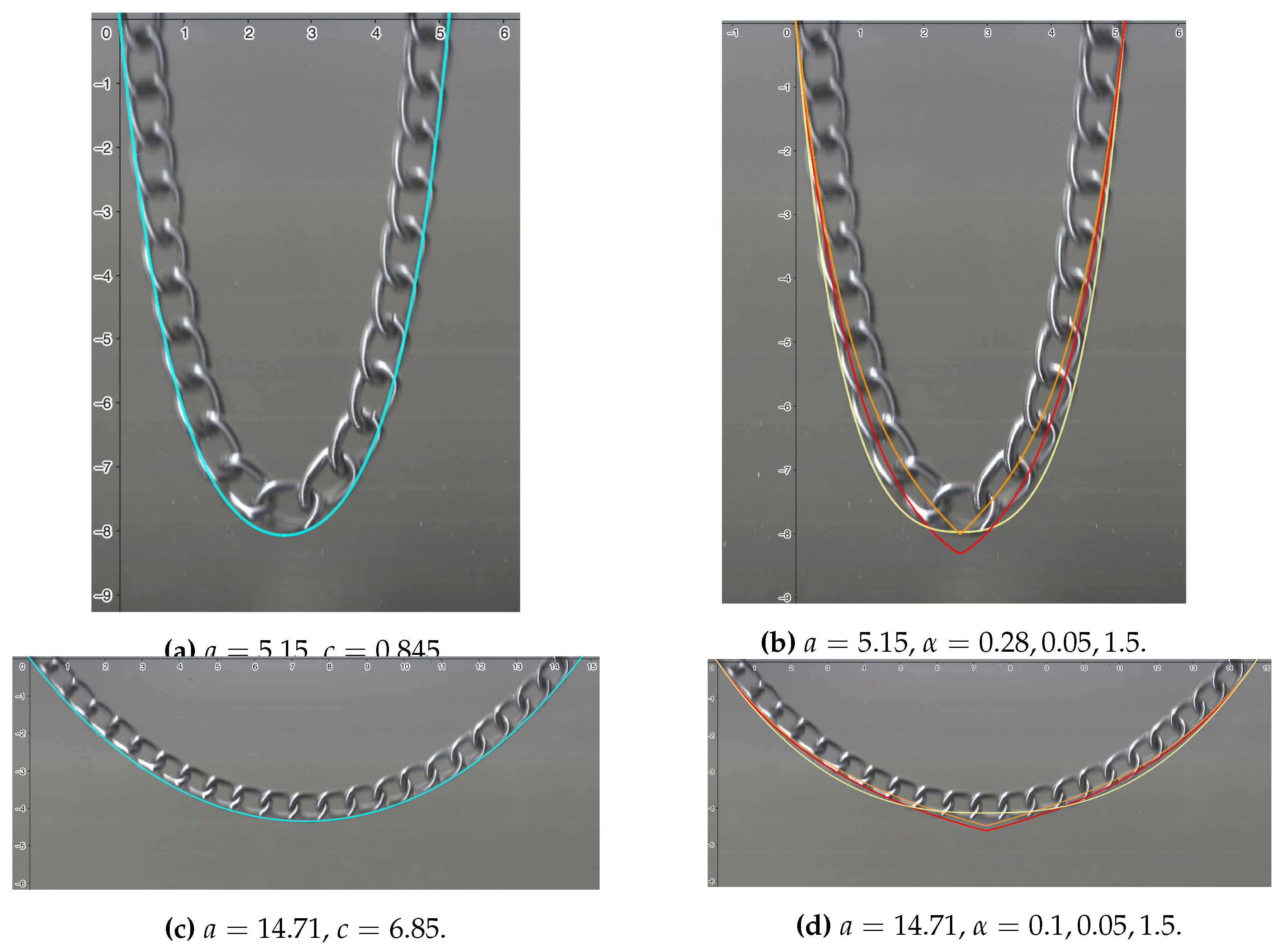
The experiment consisted of capturing several images of a hanging chain to determine the shape of the curve formed by the chain. A scanner was placed vertically with the chain positioned in front of it. When a photograph of the hanging chain is taken with a camera, the resulting curve depends on the angle of the photograph. However, this method avoids any dependence on the angle in the image.

Note that the function

y (x)

, given in (15), depends on the parameter c, which in turn depends on the linear density of the chain. The criterion we used to determine the value of c is the one that minimizes the error in approximating

y (x)

to the curve determined by the chain, taking a fixed value of the index

α

. In Figure 2 (a) and (c), the classical catenary curve is shown in blue. As we can observe from Table 1, when

α

is 1, the errors are smaller compared to the fractional case, with curves in red (

α = 0.28

c = 0.9

), yellow (

α = 1.5

c = 0.78

), and orange (

α = 0.05

c = 0.93

) when

a = 5.1

, and in red (

α = 0.1

c = 3.46

), yellow (

α = 1.5

c = 11

), and orange (

α = 0.05

c = 3.42

) when

a = 14.71

, see Figure 2 (b) and (d). Indeed, in the classical case, the error is

0.042

cm when

a = 5.15

cm and

0.028

cm when

a = 14.71

cm, considerably lower than in the fractional case, see Table 1. The errors in the figures were measured using Digimizer, an image analysis software package that allows precise manual measurements (see [14]). In this way, in Figure 2 (b) and (d), we see that the fractional curves (i.e.,

α \neq 1

) deviate from the curve determined by the chain. In other words, the fractional solution (15) does not model the curve produced by the chain.

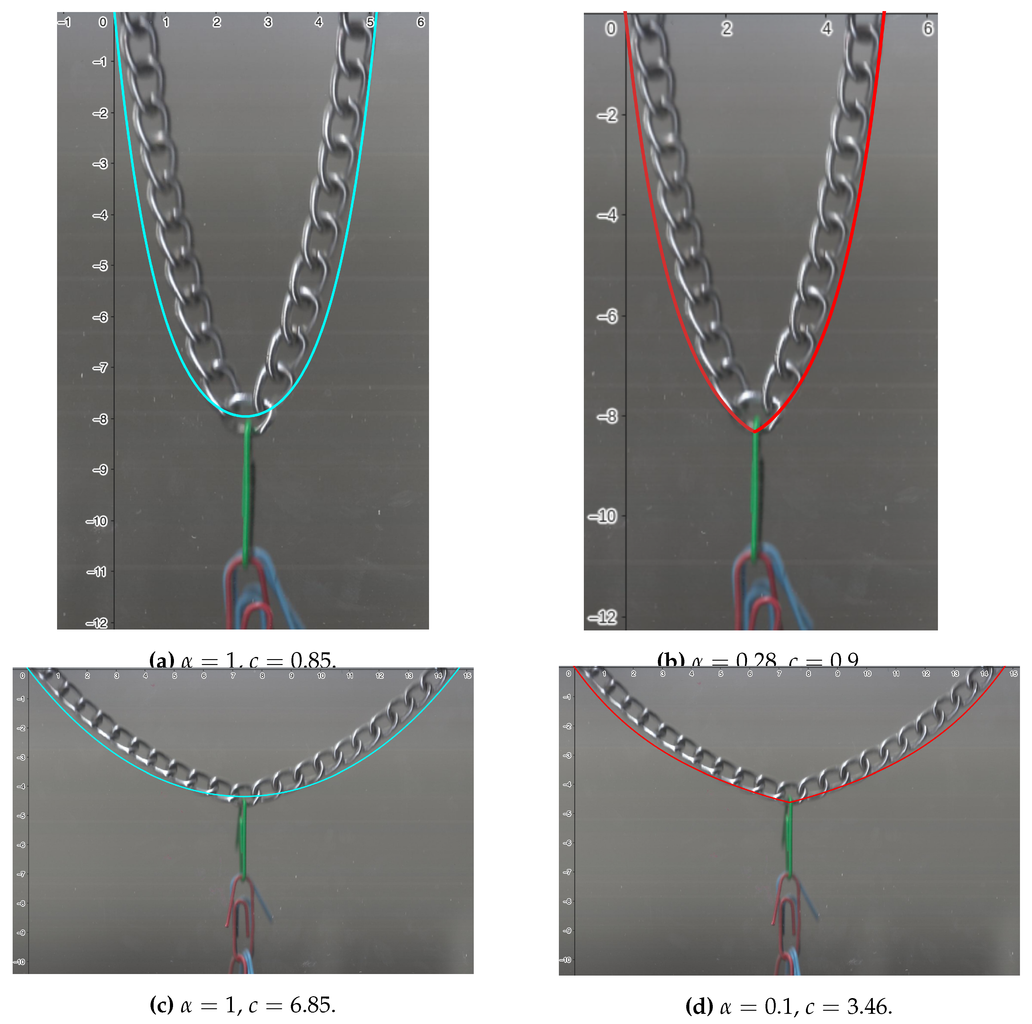
Next, we will modify the system by placing a weight of

4.344

grams at the center of the chain in both cases, i.e., for

a = 5.15

and

a = 14.71

. In Figure 3 (a) and (c), the classical curve, shown in blue, corresponds to

α = 1

. In this case, the errors are

0.258

cm when

a = 5.15

and

0.307

cm when

a = 14.71

. On the other hand, by selecting the fractional index

α

that best fits the curve, it turns out that for

a = 5.15

, the error is

0.19

cm, and when

a = 14.71

, the error is

0.16

cm, see Figure 3 (b) and (d). This means that the perturbation is better modeled with a fractional index, see (16).

It may be of particular interest to model the minimum height of the chain with the weight, as this can occur, for example, in a cable car cable. In this case, we see that the actual minimum height is

- 8.324

when

a = 5.15

. In the classical case, the error is

0.252

, and in the fractional case with

α = 0.28

, the error is

0.012

. On the other hand, when

a = 14.71

cm, the minimum height is

- 4.668

. In the classical case, the error is

0.325

cm, and in the fractional case with

α = 0.1

, the error is

0.053

. cm

6. Conclusions

It is well-known that fractional calculus is useful for modeling certain phenomena, such as temperature controllers [15] or battery charges [16]. However, we can conclude that this is not generally true. If we are studying a model with ordinary differential equations and arbitrarily introduce a fractional index, the result can produce outcomes very different from what is expected. Some authors mention that modeling with fractional calculus provides an advantage because it adds an additional degree of freedom to the system, the fractional index

α

. While this is true, it can also be the case, as in our study, that the best result is obtained by not modifying this parameter, i.e.,

α = 1

On the other hand, we have observed that fractional calculus can be useful for modeling a perturbation of the original phenomenon. In our case, the minimum height of the weighted chain is better modeled using fractional calculus. Specifically, the approximation error at the minimum point decreases by approximately twenty percent.

Author Contributions

“Conceptualization, JVM and GBG; methodology, JVM and GBG.; formal analysis, JVM and GBG; investigation, JVM and GBG; resources, JVM and GBG; writing—review and editing, JVM and GBG; visualization, GBG; supervision, JVM. All authors have read and agreed to the published version of the manuscript.”

Funding

The author GBG was supported by a Conahcyt grant. The author JVM was partially supported by the grant PIM25-2 of Universidad Autónoma de Aguascalientes.

Institutional Review Board Statement

“Not applicable”.

Informed Consent Statement

“Not applicable”.

Data Availability Statement

“Not applicable”.

Acknowledgments

The author GBG was supported by a Conahcyt grant. The author JVM was partially supported by the grant PIM25-2 of Universidad Autónoma de Aguascalientes.

Conflicts of Interest

“The authors declare no conflicts of interest.” “The funders had no role in the design of the study; in the collection, analyses, or interpretation of data; in the writing of the manuscript; or in the decision to publish the results”.

References

Luo, X.; Zhang, F.; Pu, M.; Xu, M. Catenary optics: a perspective of applications and challenges. Journal of Physics: Condensed Matter 2022, 34, 381501–381501. [Google Scholar] [CrossRef]
AutLuo, X.; Pu, M.; Guo, Y.; Li, X.; Zhang, F.; Ma, X. Catenary functions meet electromagnetic waves: opportunities and promises. JAdvanced Optical Materials 2020, 8, 2001194–2001194. [Google Scholar]
Conti, G.; Paoletti, R.; Trotta, A. The catenary in history and applications (La catenaria nella storia e nelle applicazioni). Science & Philosophy 2017, 2, 169–94. [Google Scholar]
Martínez–Jiménez, L.; Cruz–Duarte, J.M.; Rosales–García, J.J. Fractional solution of the catenary curve. Mathematical Methods in the Applied Sciences 2021, 10, 7969–7978. [Google Scholar] [CrossRef]
Eftekhari, L.; Hosseinpour, S.; Khalighi, M. A comparison between Caputo and Caputo–Fabrizio fractional derivatives for modelling Lotka–Voltera differential equations. Abbreviated Journal Name phrase indicating stage of publication (submitted; accepted; in press). 2019. [Google Scholar]
Conejero, J.A.; Franceschi, J.; Picó-Marco, E. Fractional vs. ordinary control systems: what does the fractional derivative provide? Mathematics 2022, 10, 2719–2719. [Google Scholar] [CrossRef]
Spiegel, M.R. Applied differential equations, 1rd ed.; Publisher: Prentice-Hall, New York, 1981. [Google Scholar]
Such, M.; Jimenez-Octavio, J.R.; Carnicero, A.; Lopez-Garcia, O. An approach based on the catenary equation to deal with static analysis of three dimensional cable structures. Engineering structure 2009, 31, 2162–2170. [Google Scholar] [CrossRef]
Jiang, Z.; Liu, X.; Shi, K.; Lin, Q.; Zhang, Z. Catenary equation-based approach for force finding of cable domes. International Journal of Steel Structures 2019, 19, 283–292. [Google Scholar] [CrossRef]
Ortigueira, M.; Machado, J. Which derivative? Fractal and Fractional 2017, 1, 3–3. [Google Scholar] [CrossRef]
Valério, D.; Ortigueira, M.D.; Lopes, A.M.; Author 1, T. How many fractional derivatives are there? Mathematics 2022, 10, 737–737. [Google Scholar] [CrossRef]
Kilbas, Anatoliĭ Aleksandrovich, Srivastava; Trujillo, J.J. Theory and applications of fractional differential equations, 1rd ed.; Publisher: Elsevier, 2006. [Google Scholar]
Kilbas, Anatoly A.; Marichev, O.I.; Samko, S.G. Fractional integrals and derivatives (theory and applications), 1rd ed.; Publisher: Gordon and Breach, Switzerland, 1993. [Google Scholar]
Digimizer. Available online: https://www.digimizer.
Feliu-Batlle, V.; Pérez, R.R.; García, F.J.C.; Rodriguez, L.S. Smith predictor based robust fractional order control: Application to water distribution in a main irrigation canal pool. Journal of Process Control 2009, 19, 506–519. [Google Scholar] [CrossRef]
Tian, J.; Xiong, R.; Shen, W.; Wang, J.; Yang, R. Online simultaneous identification of parameters and order of a fractional order battery model. Journal of Cleaner Production 2020, 247, 119147–119147. [Google Scholar] [CrossRef]

Figure 1. The catenary curve

Figure 2. Weightless pendant chain.

Figure 3. Weighted pendant chain.

Table 1. Different values for fractional catenary parameters, see (15).

a (cm)	$α$	c	error (cm)
	0.05	$0.925$	$0.361$
$5.15$	0.28	0.9	0.273
	1	0.845	0.017
	1.5	0.78	0.079
	0.05	$3.42$	$0.264$
$14.71$	0.1	3.46	0.241
	1	6.85	0.009
	1.5	11	0.206

Disclaimer/Publisher’s Note: The statements, opinions and data contained in all publications are solely those of the individual author(s) and contributor(s) and not of MDPI and/or the editor(s). MDPI and/or the editor(s) disclaim responsibility for any injury to people or property resulting from any ideas, methods, instructions or products referred to in the content.

© 2024 by the authors. Licensee MDPI, Basel, Switzerland. This article is an open access article distributed under the terms and conditions of the Creative Commons Attribution (CC BY) license (http://creativecommons.org/licenses/by/4.0/).

Copyright: This open access article is published under a Creative Commons CC BY 4.0 license, which permit the free download, distribution, and reuse, provided that the author and preprint are cited in any reuse.

MDPI Initiatives

Important Links

Choose an area of interest and we will send you notifications of new preprints at your preferred frequency.

Disclaimer

Erroneous Applications of Fractional Calculus: The Catenary as a Prototype

Abstract

1. Introduction and Statement of the Results

2. Classical Catenary Curve

3. Some Preliminaries on Fractional Calculus

4. Fractional Catenary Curve

5. Physical Experiments

6. Conclusions

Author Contributions

Funding

Institutional Review Board Statement

Informed Consent Statement

Data Availability Statement

Acknowledgments

Conflicts of Interest

References

MDPI Initiatives

Important Links

Subscribe