
You are currently viewing a beta version of our website. If you spot anything unusual, kindly let us know.
Preprint
Article
Flood Segmentation: Self-Supervised Knowledge Transfer from Optical to SAR
Altmetrics
Downloads
133
Views
74
Comments
0


This version is not peer-reviewed
Abstract
Our world is increasingly challenged by managing the impacts of natural disasters, particularly floods, which are frequent, dangerous, and costly. Traditional flood mapping methods, reliant on Optical satellites (MSI), struggle under cloud cover which is typical during such events. Synthetic Aperture Radar (SAR) offers a promising alternative with its cloud-penetrating capability, though its use has been limited due to complexity and data labeling challenges. This project aims to develop a SAR-based flood segmentation model that can rapidly and accurately map floods globally, with high adaptability to different flood types and regions. By utilizing deep learning and a novel transfer-learning technique that combines the strengths of Optical/MSI and SAR data, the model seeks to bypass the challenges of manual labeling and improve mapping accuracy. Initial results show the model's effective generalization across various flood events, with superior performance indicated by an Intersection over Union (IoU) of 0.72, outperforming existing methods and demonstrating promising capabilities in precise flood mapping.
Keywords:
Subject: Computer Science and Mathematics - Artificial Intelligence and Machine Learning
1. Introduction
Floods are increasingly threatening due to climate change, posing significant risks to lives, property, and infrastructure [1]. Effective flood mapping, crucial for disaster response, necessitates rapid and precise techniques. Preventive and emergency measures are essential for mitigating flood impacts [2]. Satellite data, particularly from Multi-Spectral Imaging (MSI) and Synthetic Aperture Radar (SAR), play a key role in near real-time flood mapping, aiding effective decision-making. While MSI usability is limited by cloud cover, SAR can penetrate clouds, providing reliable data even in adverse weather conditions. When it comes to Deep Learning, the application of SAR in flood mapping remains limited due to data scarcity and high costs of manual labelling. Our project aims at developing an automated, reliable flood mapping model using SAR, enhanced by MSI through an innovative transfer-learning approach. This model seeks to deliver accurate flood maps across multiple regions and under various conditions to improve disaster response capabilities.
In recent years, Synthetic Aperture Radar (SAR) polarimetric data has been a valuable tool in the field of flood mapping due to its unique capabilities and advantages. SAR operates by emitting radar signals towards the Earth’s surface and measuring the return signals (process known as backscattering) [3]. While traditional optical sensors, using visible light, can be interpreted by human eyes, SAR requires a different mindset. Objects on the Earth’s surface scatter the radar signals in different ways based on the object’s dimension, shape and material, allowing to differentiate various types of terrain and objects [3]. Water, with its high dielectric constant, tends to scatter all incoming radiation in a specular direction [4] when the surface is flat. This typically results in very low backscattering signals from such areas, a characteristic that is particularly useful for mapping floodwaters over non-flooded areas using SAR intensity images. In our project we will make use of the ESA Sentinel-1 constellation from Copernicus, which is an European Union program aimed at monitoring the Earth. Our focus will primarily be on the intensity features of the imagery, for which we will exclusively use the Ground Range Detected (GRD) products from the Sentinel-1 mission. GRD products are pre-processed images which are lighter and do not include phase information, but they retain the intensity feature, which is crucial for differentiating between water and land surfaces [5]. Historically, most SAR applications for flood segmentation have been using statistical thresholding to discriminate between water and non-water pixels [6,7]. Only recently, with the advance in Machine Learning (ML), new models are increasingly being adopted [8]. Among these, Convolutional Neural Networks (CNNs) are particularly prominent for image recognition tasks, offering significant improvements over traditional threshold-based methods for flood segmentation. Unlike threshold approaches that rely on individual pixels, CNNs consider the context provided by neighboring pixels. We will explore the details of these advancements in the subsequent sections.
2. Thresholding
Numerous flood models in the literature have been using thresholding techniques like Otsu thresholding [9] to differentiate water from land surface, which in contrast has an higher backscatter signal; Otsu thresholding in simple terms, finds the best thresholding value to separate the two distributions. However, this is not always possible, in fact in some cases, the two distributions are indistinguishable and are mixed in one single bell curve; in such cases the Otsu method fails to detect the optimal threshold. Many approaches try to solve this problem by applying local thresholding techniques [10]; in [11] an iterative algorithm searches for tiles of variable sizes to find a local threshold that can better distinguish the distributions of the two classes. These methodologies have been widely used, but they struggle in challenging areas where the backscatter values resemble those of water such as asphalt, dry regions, radar shadows, or ice and snow, which in turns gives many false positives [12]. To account for the cases where the thresholding approaches fail, recent approaches exploit spatial information of adjacent pixels [13]. In SAR images, neighbours pixels often exhibit similar values, the spatial information refers to the information that can be gathered by exploiting adjacent pixels to distinguish structure, texture, and features present in the image. In the next section we will delve into deep learning models and see how they can exploit the spatial information to better delineate flood areas.
3. Deep Neural Networks
Deep learning models have become more and more popular nowadays and are constantly evolving. They are also increasingly being applied in recent research, including for tasks such as flood segmentation. Notably [8] does an overview of existing deep learning methods for flood segmentation, and it suggests the preference towards specific model architectures based on their “inductive biases”. The inductive bias refers to the set of assumptions a learning algorithm makes or is expected to make to predict outputs (labels) based on inputs (features). Based on the assumption that in flood analysis, SAR data often exhibit spatial correlations between adjacent pixels, NN (Neuronal Network) layers can be configured to exploit these data structures, by introducing constraints on the connections and interactions between inputs and outputs and favouring certain model architectures over others [8]. One way to exploit spatial information is the use of a convolutional layer, which is the core component of Convolutional Neural Network (CNN).
3.1. CNN (Convolutional Neural Network)
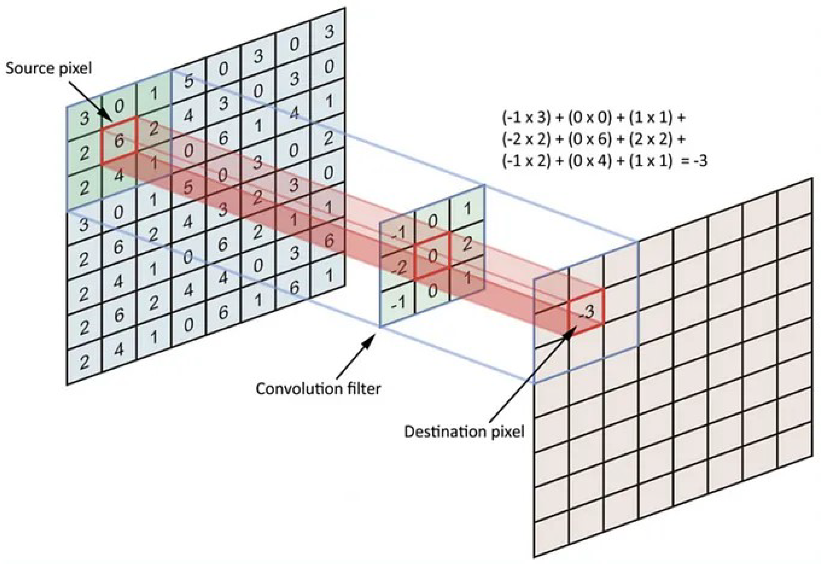
Convolutional Neural Networks (CNNs) are a type of model in the field of deep learning, particularly useful at processing data with a grid shape, such as images. Central to CNNs are convolutional layers, which exploit spatial information by capturing the local relationships among pixels through the use of filters. In a convolutional layer, traditional neuron weights are replaced with filters. These filters compute new values for each pixel by considering the local relationships with its neighbors. The architecture is designed to progressively abstract higher-level features from the raw input in the initial layers to more abstract representations in deeper layers, making CNNs particularly powerful for tasks like image classification.
Figure 1.
Illustration of the convolutional operation, visualized through a 3x3 kernel applied to an input image, that produces a feature map highlighting detected patterns. This process, core of CNNs, enables the network’s to automatically learn spatial relationships of features [14].
Figure 1.
Illustration of the convolutional operation, visualized through a 3x3 kernel applied to an input image, that produces a feature map highlighting detected patterns. This process, core of CNNs, enables the network’s to automatically learn spatial relationships of features [14].
3.2. Segmentation Models: An Overview
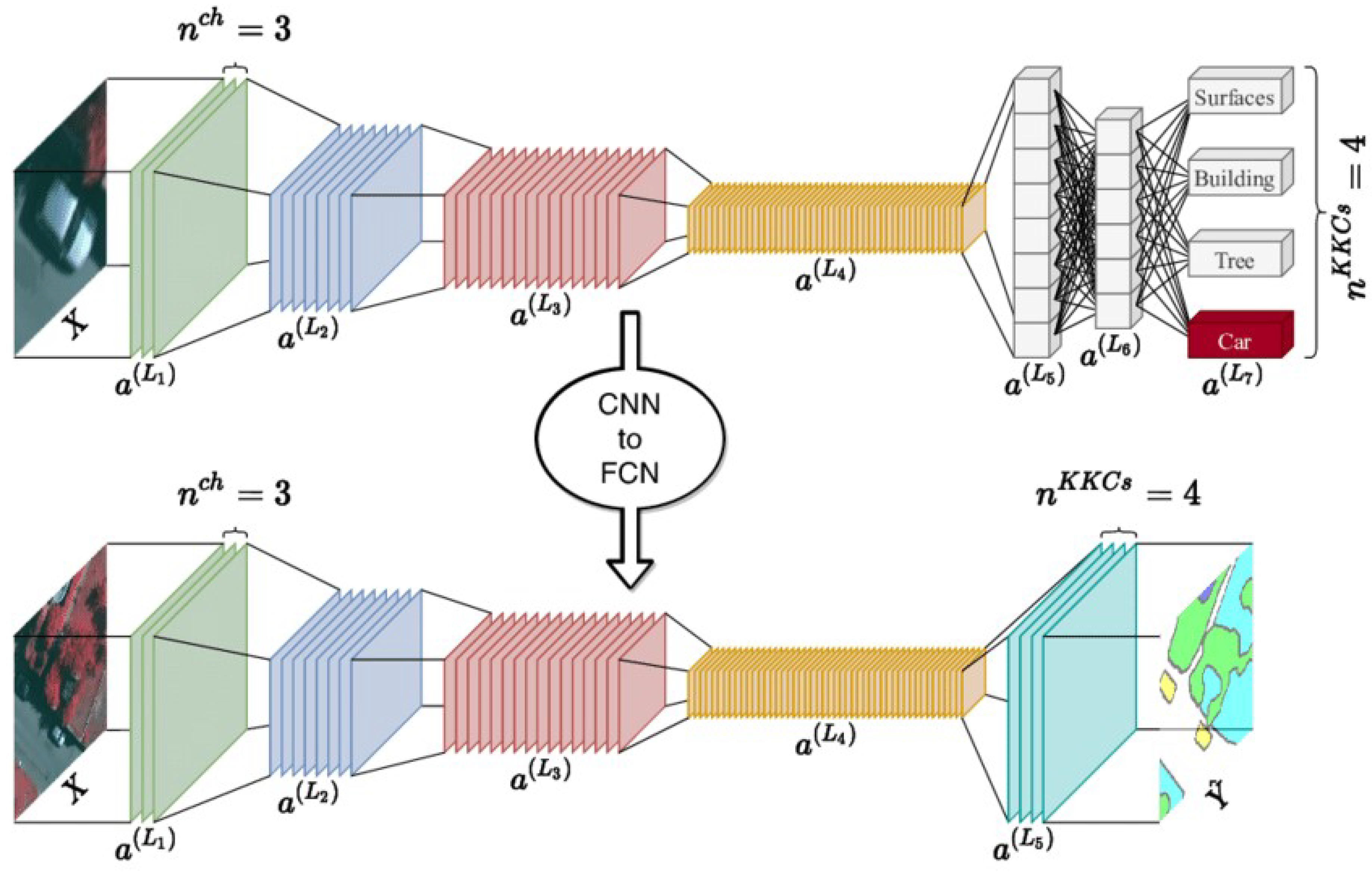
The standard CNN architecture can’t be directly used for image segmentation. In fact, as shown in Figure 2 the fully connected layers link the pooling layers to a 1D output, which loses spatial context. To retain the spatial context in the output layer, other segmentation specific architectures have been proposed in the literature. The Fully Convolutional Network (FCN) introduced in [15] utilizes pre-existing CNN architectures designed for classification tasks (such as AlexNet, VGG, etc.). These architectures are adapted into fully convolutional networks and their learned representations are transferred to the segmentation task through fine-tuning. FCNs introduced the idea of replacing fully connected layers with convolutional layers, to produce pixel-wise predictions for segmentation. The architecture consists of an encoder path, which downsamples the input image to extract features, and a decoder path, which upsamples the features to produce the segmentation map. FCNs have been effectively applied in tasks such as flood segmentation, as demonstrated in [16].
Figure 2.
Abstract view of a CNN architecture for classification tasks. Following convolutional and pooling layers, the network typically ends with fully connected layers that integrate these learned features into predictions or classifications, outputting a one-dimensional array corresponding to the classes [14].
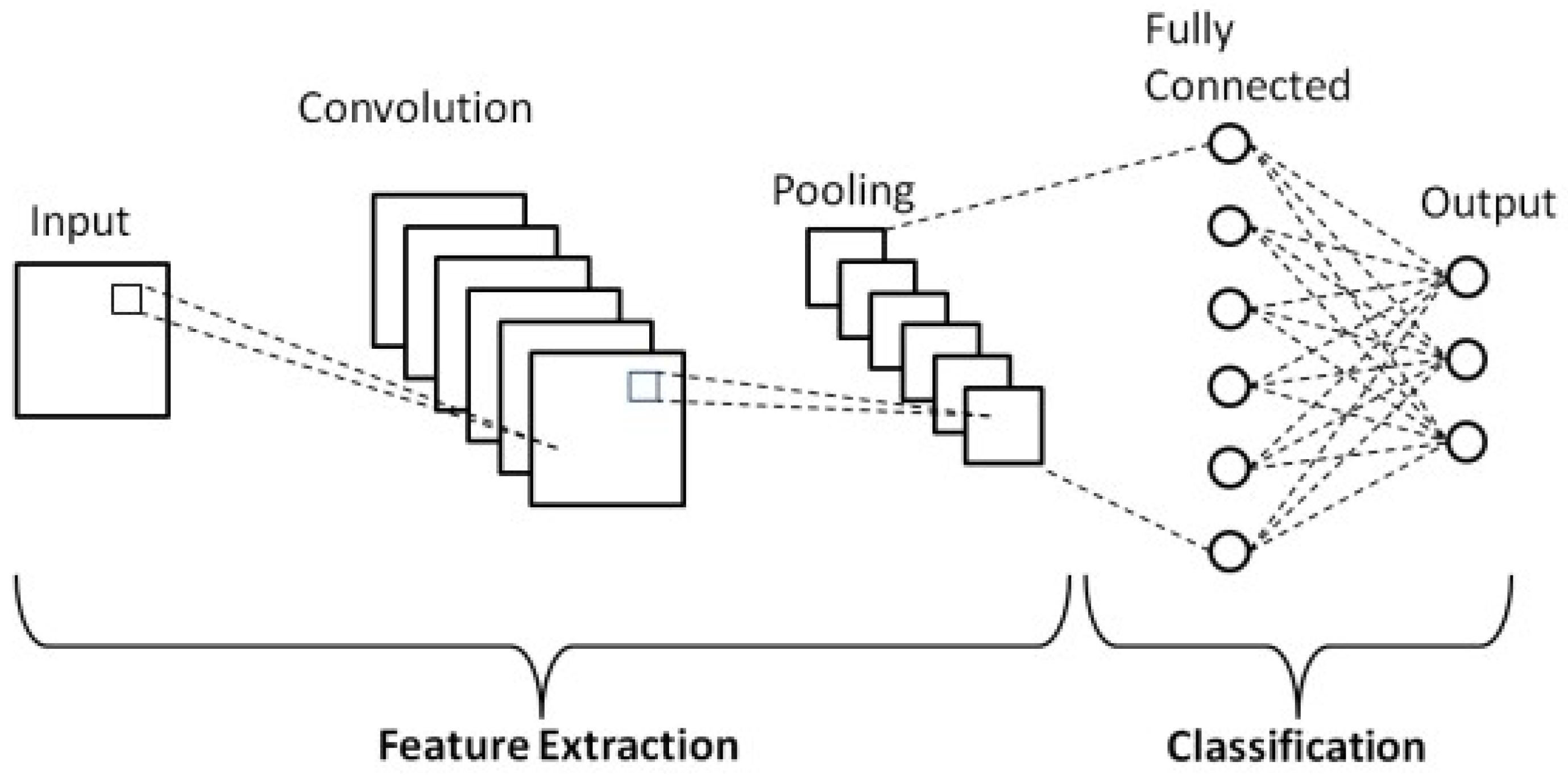
Figure 3.
Architecture example of a CNN for image classification and its equivalent FCN architecture with the same backbone for semantic segmentation. KKCs = 4 refers to the number of output classes (channels) probabilities for pixel wise predictions. We can see that in the FCN, the fully connected layers are replaced by convolutions to produce pixel-wise predictions [17].
In 2015, a novel paper [18] proposed the U-Net architecture which builds upon the ideas introduced by FCNs but adds the concept of skip connections. The idea behind it is that each encoder and decoder layer is symmetrically linked with a skip connection, that is achieved by concatenating the output from encoding layers to corresponding decoding layers. The goal was to provide a more detailed segmentation mask by exploiting global and local features of an image. This concept, initially proposed in [18], was further reproposed a few months later by a new model architecture called ResNet (Residual Nets) [19]. ResNet builds upon the concept of skip connections from Unet [18] but approaches it from a different angle. ResNet [19] solves a common issue encountered in deep neural networks: as the network gets deeper with more layers, the gradient (used to update the weights based on the error) diminishes significantly during backpropagation, leading to difficulties in updating the weights of earlier layers. This is known as the gradient vanishing problem. Recent advances in segmentation combine the power of ResNet deep features extraction into the Unet Encoder, which significantly improve the segmentation performance. This hybrid architecture has been applied for sea-land optical segmentation in [20], demonstrating that replacing ResNet into the Unet architecture significantly improves feature representation. This enhancement, together with fully connected Conditional Random Fields (CRFs) as post-processing predictions refinement, leads to more accurate delineation of coastlines and better-preserved regions in sea-land segmentation tasks as shown in [20].
3.3. Conditional Random Fields (CRFs) in Segmentation
Conditional Random Fields (CRFs) have been widely used as a post-processing technique to refine segmentation results. Initially developed as a probabilistic framework for segmenting and labelling sequential data [21], CRFs were later adapted into fully connected CRFs to address the challenges of semantic segmentation. However, the widespread adoption of fully connected CRFs was slowed down by the computational demands of their inference processes. The scenario changed with the introduction of an efficient inference algorithm shown in [22], making fully connected CRFs more efficient and viable for practical use especially as a common technique for post-processing in segmentation tasks. By modelling the spatial dependencies between pixels, CRFs improve the coherence and accuracy of the segmentation output, particularly in distinguishing between closely related classes and preserving boundary definitions. Their application, combined with advanced neural network architectures like U-Net and ResNet, represents a comprehensive approach to tackling complex segmentation tasks with improved precision. Notably in [20], it is demonstrated that the use of CRF as a post-processing stage enhances the segmentation predictions results. In our research, we adopt the U-Net architecture integrated with an encoder block derived from the ResNet encoder. Furthermore, our exploration will include the application of CRFs, in alignment with current trends indicated in the literature.
4. Unsupervised Models for Flood Segmentation
The complexity and cost of data retrieval, preprocessing, and manual labeling make building a new dataset from scratch difficult, emphasizing the need for unsupervised approaches. To address these current dataset limitations, several papers have proposed self-supervised or fully unsupervised techniques for flood segmentation. These approaches eliminate the need for manually labeled datasets, which are expensive, labor-intensive and not always accurate.
4.1. Fully Unsupervised Learning
CLVAE [23] proposed an unsupervised model based on change detection to detect floods, which is reported to achieve an Intersection Over Union (IoU) of 64.53%. Their architecture is composed of a Variational Autoencoder (VAE) with a Contrastive Learning loss to automatically extract and learn latent distributions from images. The model is trained on mixed patches of floods from Sen1Floods11 [24] and MMFlood [25] dataset. Their approach is to apply a VAE model to both pre- and post-flood images, and compute the difference on their latent distributions. Then, based on a manually selected threshold, the flood over non-flood pixels are classified. Although this approach solves the need for labels, it comes with some limitations. The VAE architecture is traditionally designed to extract latent distributions of entire images, presenting challenges when applied for pixel-level segmentation tasks. Since it’s unpractical to apply the VAE model to single pixels, their proposed solution involves utilizing extremely small patch sizes of 16x16 so that the classification is conducted in these entire blocks of 16x16 pixels. This approach inevitably results in the loss of valuable spatial information, which is reportedly addressed by Reflective Padding [23]. Additionally, because the model isn’t specifically fine-tuned for any task after its initial unsupervised training, their technique might identify various changes, not necessarily changes from no flood to flood.
Even though fully unsupervised classification techniques are gaining popularity, there remains a significant gap in their application for unsupervised pixel-level tasks for semantic segmentation.
4.2. Semi-Supervised Learning
Other approaches rely on semi-supervised learning. To solve the problem of large unlabelled dataset, [26] uses an ensemble of models in a cyclical approach. The dataset used is from the Emerging Techniques in Computational Intelligence (ETCI). An U-net model is firstly trained on a small set of labelled data. The model is used to produce pseudo-labels from the large unlabelled data. In a second stage, an ensemble of Unet and Unet++ models are trained from scratch both on the first labelled data and pseudo-labels generated from the previous step. The training cycle is repeated until the performance improvement plateau. Their segmentations are then postprocessed with CRF, In line with the previously cited paper [20]. They report to achieve an IoU of 0.68 on the first round of iteration and an IoU of 0.76 at the end of the iterative training. However, this method presents several challenges. Their hold-out test set contains only patches from a single flood event in Florence, Italy, and has yet to be tested in other regions, therefore it’s still unclear its performance and generalization on different regions. Furthermore, their iterative method repeatedly uses the predictions from the previous model as ground truth, therefore there isn’t sufficient evidence that these pixels are accurately classified since they still originate from the same model predictions.
4.3. Transfer Learning
While the earlier method faces limitations in terms of the need for manual annotations and the potential inaccuracies in the pseudo-labels. DeepAcqua [27] eliminates the need for manual annotations by employing a teacher-student model, where the Normalized Difference Water Index (NDWI) from paired Optical images serves as the teacher to automatically generate labelled data for training the SAR model (“student”). This approach avoids the reliability issues associated with pseudo-labels since it does not rely on the same model predictions for generating training data. Instead, it relies on the accuracy of a distinct mathematical index derived from another satellite, Sentinel-2 (Optical). However, it’s worth noting that their methodology is not exclusively applied toward flood-related tasks but rather is focused to wetlands in general. Our approach is built upon an expansion of this methodology. Instead of utilizing the NDWI index as the teacher model, we directly incorporate the water classifications offered by Copernicus in Sentinel-2 Optical bands. Specifically, we leverage the Scene Classification Layer (SCL) [28], which has demonstrated superior accuracy in detecting water compared to the standard NDWI, to train the SAR based model.
5. Novelty
We introduce a novel framework aimed at improving flood mapping capabilities through the combined use of SAR and MSI. SAR, known for its ability to penetrate cloud cover, can provide reliable acquisitions when optical satellite (MSI) data are not available. At the core of this project is the development of a novel transfer-learning framework that exploits the more precise MSI or Optical modality to transfer knowledge to SAR models. Inspired by previous studies we adopt a teacher-student model, similar to DeepAcqua [27], but using Scene Classification Layer (SCL) instead of the Normalized Difference Water Index (NDWI). Specifically, our framework incorporates the U-Net architecture with ResNet encoder blocks. Moreover, recognizing the limitations of current datasets and the challenges in manual labeling, we train our model on a new dataset, consisting of both floods and water regions. This dataset covers a variety of regions worldwide, ensuring the generalization of our model across different geographical and environmental scenarios.
6. Materials and Methods
6.1. Dataset Creation
The Copernicus Programme, through Sentinel satellites, provides free access to satellite data, including Sentinel-1 SAR data. Pre-processing steps are necessary to improve image quality. The article in [29] discusses the challenges and necessary steps involved in preprocessing Sentinel-1 Ground Range Detected (GRD) data. MMFlood [25] uses the Sentinel Hub API, which aggregates multiple satellite data, enabling real-time processing and access to specific AOIs within seconds, thus avoiding extensive preprocessing.
A significant challenge in building the training dataset is the precise and reliable delineation of flood areas, as most flooded pixels are usually selected manually or adjusted based on operator knowledge. The Sen1Floods11 dataset [24] comprises Sentinel-1 and Sentinel-2 data, with 446 labeled 512x512 chips covering 11 flood events, but it does not consider various flood types and relies on human intervention, introducing potential errors. MMFlood [25] uses the Copernicus Emergency Management Service (EMS) to retrieve flood delineations in vector files for their dataset, consisting of 8,522 labeled 512x512 patches from Sentinel-1, covering 95 flood events globally. EMS has operated since 2021, providing maps for environmental disasters based on a closed-source algorithm and then reviewed by humans, but their labels are not always accurate.
Following the approach in [25], we use the Sentinel Hub API to directly obtain satellite products. We then pair Sentinel-1 and Sentinel-2 images to create a new dataset, SAR-Optical, for training our model. Since the dataset only contains uni-temporal flood and permanent water patches, we create a new dataset derived from the MMFlood dataset [25], enhanced with pre-flood images, which we call MMFlood-CD (change detection). This will be used to qualitatively assess the model performance on flood events through change detection.
6.1.1. Images Acquisition and Preprocessing
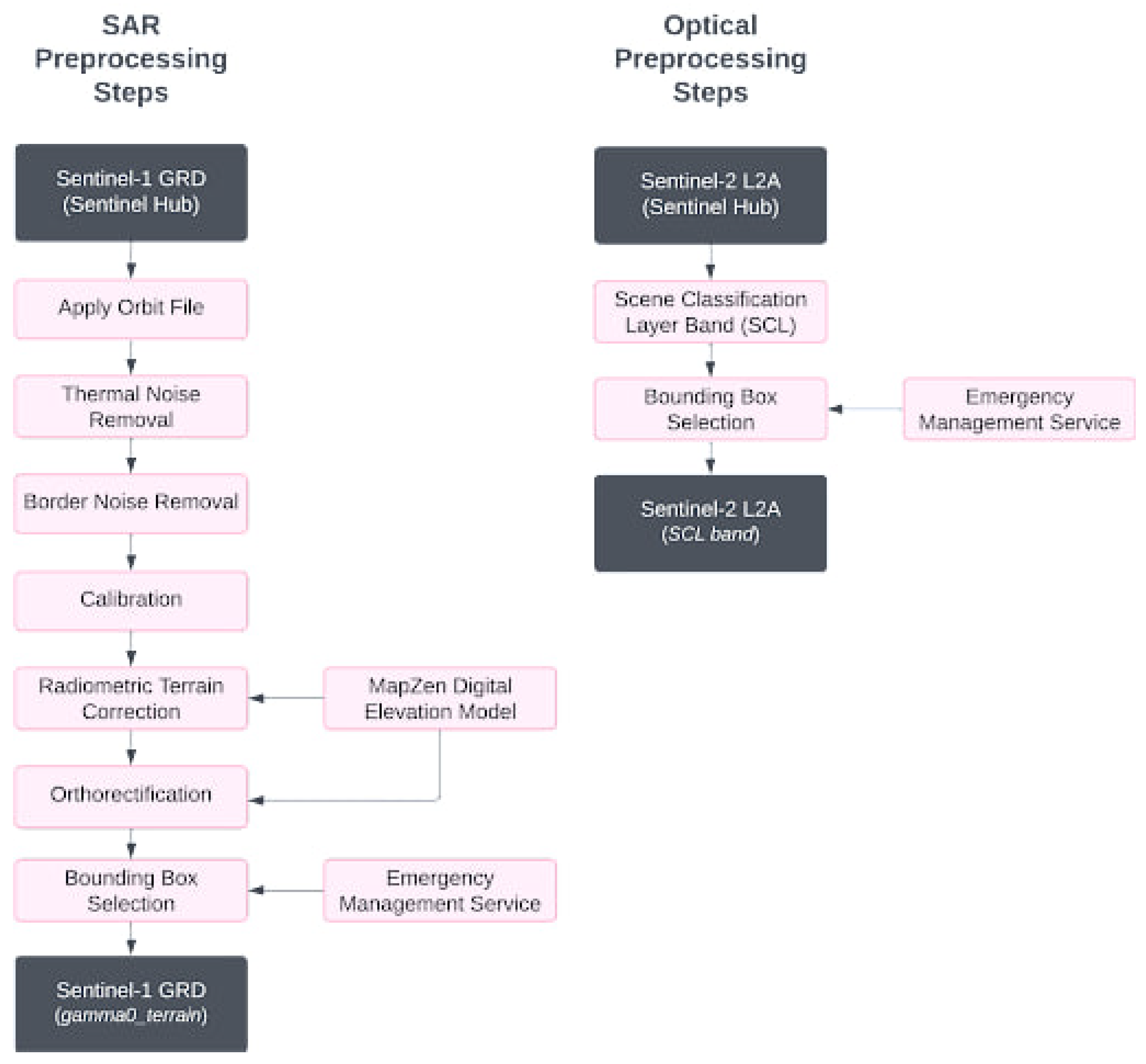
With the use of Sentinel Hub API, we can specify the pre-processing steps directly in the parameters of the requests. In our experiments we use Ground Range Detected (GRD) imagery, which preserves signal amplitude while eliminating phase information and reducing speckle noise through multi-look processing [29]. All the images are provided with a spatial resolution of 20 m and a pixels spacing of 10 m, and have a 32-bit floating point precision. As per preprocessing steps, we apply calibrations and thermal noise removal as outlined in the standard workflow proposed in [29]. Moreover, we apply Radiometric Terrain Correction (RTC) and Orthorectification using the MapZen Digital Elevation Model to more accurately geocode the images. We purposely avoid applying speckle filtering, based on the hypothesis, aligned with the findings of [25], that CNNs models inherently possess the capabilities to smooth images to extract relevant information.
6.1.2. SAR-Optical
The SAR-Optical dataset contains paired SAR and Optical patches, and it is used to train the SAR model using the Optical ground truth. The image pairing was not straightforward, since it’s unusual to have both Optical and SAR images taken on the same day, we made sure that the Optical image acquisitions were taken within a maximum of three days after the flood event. This is a good compromise that allows a balanced number of samples while accounting for rapid changes in floods. Clouds may obstruct the regions of Interest (ROIs), therefore we selected only those that don’t have clouds and that have at least 0.01% of water pixels. The Optical ground truth is derived from the SCL layer contained in the Sentinel-2 L2A Optical product, provided directly by Copernicus. Their layer automatically classifies various land covers such as water, land, clouds, etc., and is consistently updated. We extracted only the water classification from this layer to generate a binary raster image that marks pixels as 1 where water is present and 0 where it is not. Unlike the approach taken by DeepAcqua [27], we opt for the SCL layer as it presents a more reliable alternative to the NDWI calculation, which can occasionally miss water regions.
Figure 4.
Summary of the preprocessing steps involved to prepare the GRD and Optical products applied directly in Sentinel Hub. The API accounts for both data retrieval and preprocessing.
Figure 4.
Summary of the preprocessing steps involved to prepare the GRD and Optical products applied directly in Sentinel Hub. The API accounts for both data retrieval and preprocessing.
6.1.3. MMFlood-CD
The MMFlood-CD dataset contains the same flood events delineations and naming conventions of MMFlood dataset [25], with the addition of pre-flood images. This dataset is utilized solely for a qualitative visual comparision of our SAR model with the EMS ground truth, included in MMFlood-CD. Given that the objective of the SAR model is to detect water, regardless of it being floodwaters or permanent water, we take advantage of both pre- and post-flood images and use a change detection module to detect flood. A more detailed explaination of this process can be found in Section 6.4.
In the following table a summary of the 3 datasets discussed in the previous sections with a comparison highlighting the differences.

Table 1.
Dataset Comparison
| Dataset | N. Events | Ground Truth | Pre-Flood Images | Labels |
|---|---|---|---|---|
| MMFlood | 1,748 | EMS | No | Flood |
| MMflood-CD | 1,748 | EMS | Yes | Flood |
| SAR-Optical | 823 | SCL Optical | No | Water and Flood |
6.2. Training Pipeline
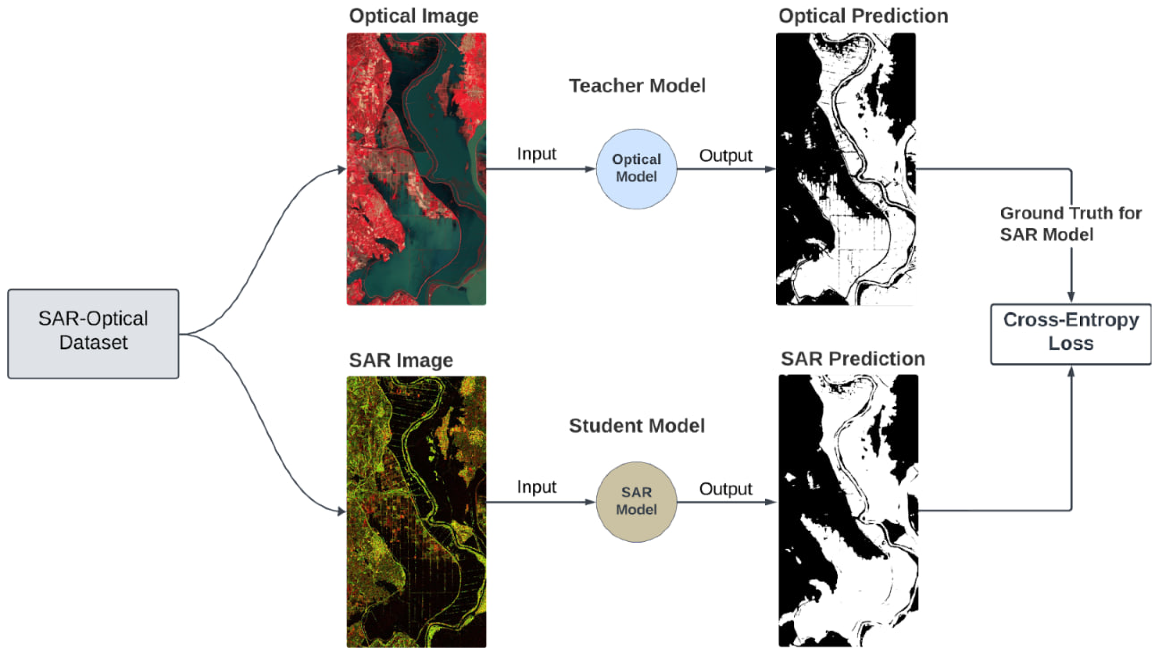
The task of flood delineation involves categorizing each pixel within an image as either flood or non-flood (background). Specifically, we define a collection of image pairs, x, where each pair, , consists of SAR images with uniform dimensions . These images are paired with corresponding labels, , also of the same dimensions, derived from optical images that serve as the ground truth. For every pixel i, its label can be either 0 or 1, with 0 indicating non-flood (background) regions and 1 indicating flood-affected areas. The goal of binary segmentation training is to develop a model, , parameterized by , which accurately predicts flood pixels across the image, mapping the input, SAR image, to a corresponding label, . Here, denotes the output of the model, represented by a matrix of size containing the raw scores (logits). These scores are subsequently converted into probabilities using a SoftMax function. Further details on SoftMax functionalities can be found in Section 6.4. The model is trained on the labels from the SAR-Optical dataset, which contains SAR images paired with the Optical ground truth. The Optical SCL Layer transfers the knowledge to the SAR model through a weighted cross-entropy function that minimizes the difference in the distributions of the two models output, making the SAR model predictions as close as possible to the Optical one.
Figure 5.
The paired Optical and SAR image, to facilitate the understanding of the SAR-Optical dataset structure. The dataset contains paired Optical and SAR images. The Optical image contains the SCL band from Sentinel-2 mission, Copernicus. This band provides a classification of the water extent which will be used as ground truth to train the SAR model.
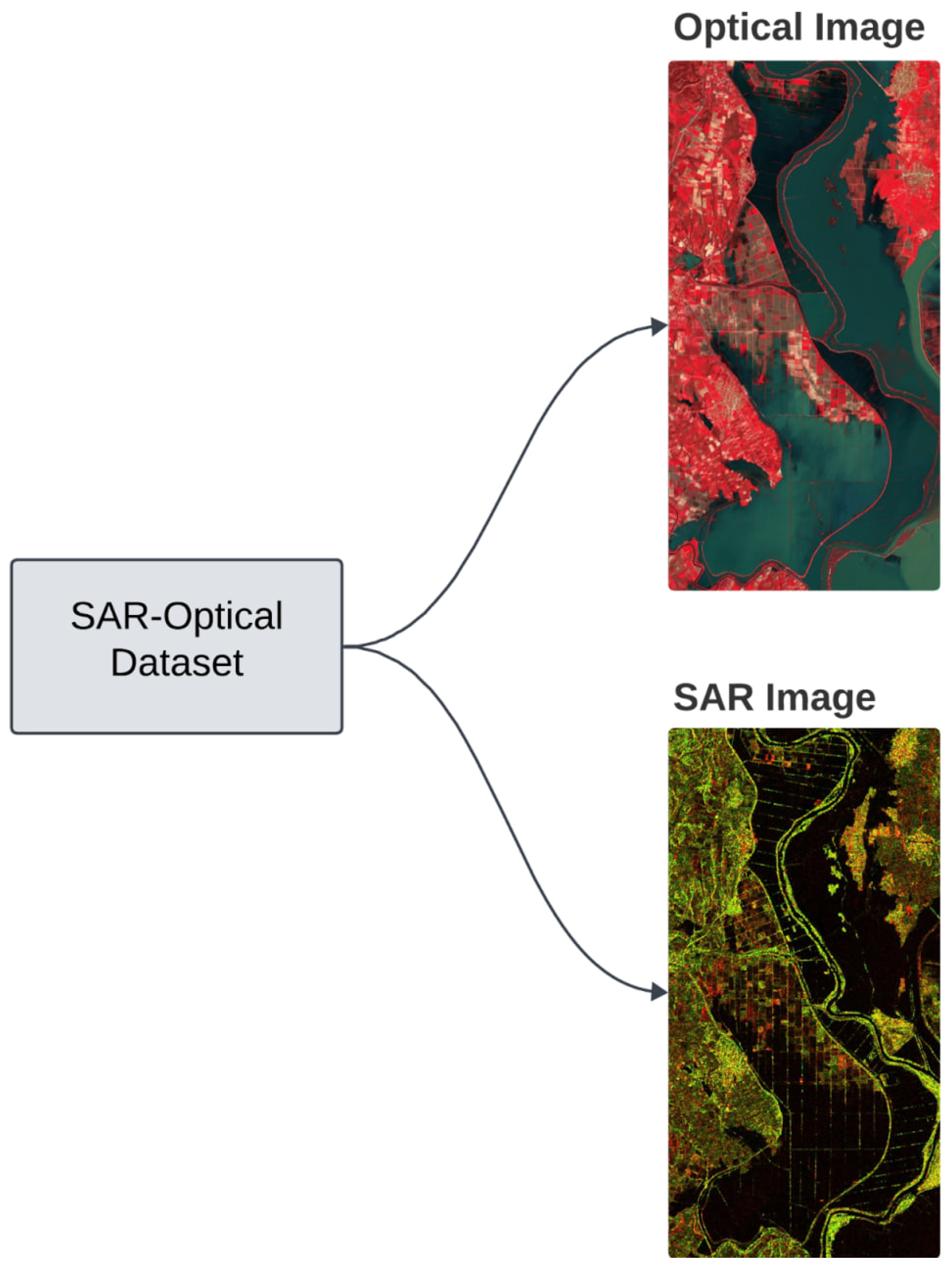
Figure 6.
Diagram to facilitate the understanding of the MMFlood-CD (CD stands for change detection) dataset structure. The dataset contains the same flood events delineation from MMFlood but with the addition of pre-flood. It also contains the EMS ground truth, that will be used just to qualitatively compare our model with their performance
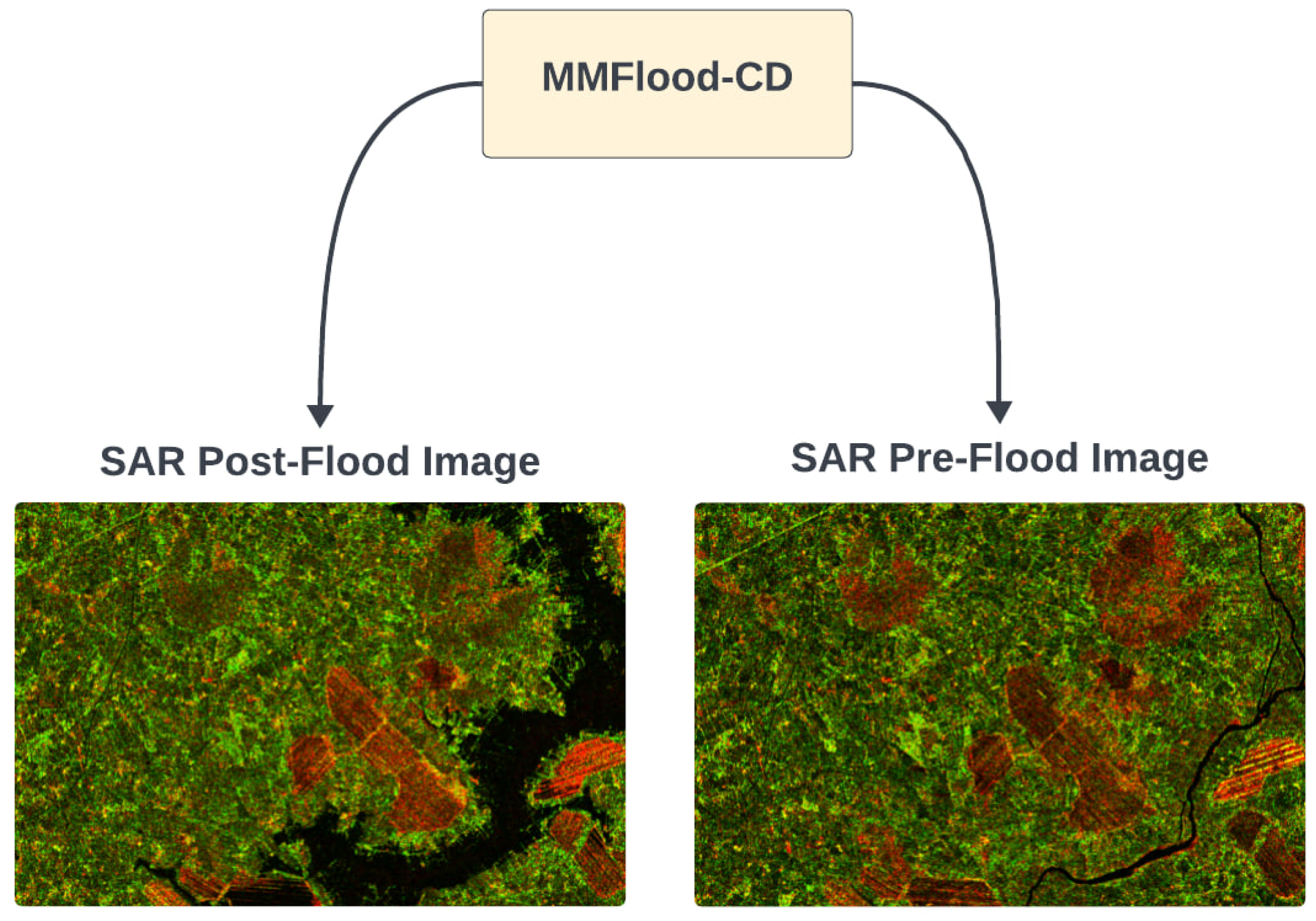
Figure 7.
Diagram of the training pipeline. The SAR model is trained on the paired SAR-Optical dataset. The predictions generated from the Optical Model are used as ground truth for the SAR Model, with the use of a Cross-Entropy Loss function.
Figure 7.
Diagram of the training pipeline. The SAR model is trained on the paired SAR-Optical dataset. The predictions generated from the Optical Model are used as ground truth for the SAR Model, with the use of a Cross-Entropy Loss function.
6.2.1. Loss Functions for Data Imbalance
We observed a significant imbalance with a water-to-land ratio of 1:11. To tackle this imbalance without altering the dataset with down sampling or up sampling techniques, we opted for specific loss functions that mitigate this issue by adjusting the weights between water and non-water classes. We explored two specific loss functions for this purpose: Focal Tversky Loss [30] and Weighted Cross-Entropy Loss.
6.2.1.1. Weighted Cross-Entropy Loss
The Weighted Cross-Entropy Loss is an adaptation of the standard Cross-Entropy Loss, introducing a weighting factor to account for class imbalances. This is particularly useful in datasets where one class is significantly more frequent than the other, which can lead to a model bias towards the majority class. The weighted version is defined as:
Here, w represents the weight assigned to the positive class. This weight is typically set inversely proportional to the class frequencies, meaning that a higher weight is assigned to the less frequent class. This adjustment aims to amplify the loss contributed by the minority class, encouraging the model to pay more attention to correctly classifying these instances.
6.2.1.2. Focal Tversky Loss
In our experiments, inspired from previous studies [25,31] we also explored the Focal Tversky Loss [30], which unlike the traditional Cross-Entropy Loss, aims directly at optimizing the Intersection over Union (IoU) score, aligning closely with our segmentation objectives. The Focal Tversky Loss is defined as:
Here, represents the Tversky index, and is a modulating factor parameter that diminishes the influence of easily classified examples, thereby making the model focus more on hard to classify examples. The Tversky index is a generalization of the IoU metric that introduces two parameters, and , to control the relative importance of false positives and false negatives. Specifically, is given by:
In this formula, , , and stand for true positives, false positives, and false negatives, respectively. This loss is specifically designed to account for the imbalance in the labels, in this case between water and non-water classes, by applying a dynamic balancing mechanism. The weighting factor for water and for non-water moderates the significance of respective pixels, with a higher emphasizing water pixels
6.3. Model Architectures
We investigated various model architectures to establish benchmarks. Our approach involved testing different combinations of encoders and decoders to assess their efficiency. Initially, we assessed the performance of U-Net with its standard encoder. Subsequently, we experimented by replacing the U-Net encoder with other backbones encoders similar to those described in [25,27]. Alongside the U-Net decoder, we assessed various encoders, with ResNet-50 exhibiting superior performance. A detailed comparison of these models is provided in Section 7.0.2. In our implementation of the Unet with the ResNet-50 encoder, we use batch normalization to consistently accelerate the convergence of deep networks [32]. ReLU activation functions are employed within each residual block, alongside the skip connections that add the input of each block to its output. This mechanism facilitates more direct flow of gradients, as detailed in Section 3.2. The encoder part of our U-Net, which uses the ResNet backbone, progressively down-samples the input image, capturing increasingly abstract representations of the data at different scales. Each stage in the ResNet-50 encoder corresponds to a specific feature map size and depth, with the number of filters doubling as the spatial dimensions halve, starting from 64 filters in the first stage to 2048 filters in the final convolutional stage. This approach expands the search space and improves the network’s learning ability, resulting in an increase in trainable parameters. For the U-Net with ResNet-50 architecture, this amounts to around 23 million parameters.
6.4. Change Detection Module for Flood Analysis
Our model is designed to identify areas covered by water, without specifically distinguishing between flooded and non-flooded regions. To highlight the extent of flooding, we compute the difference between the predictions made before and after the flood event, through the pre- and post-flood images. The model’s predictions are first processed through a SoftMax function to convert the raw logits from the output layer into probabilities. The SoftMax function in simple terms, is a mathematical operation that transforms a vector of real-valued logits into a vector of probabilities by exponentiating each logit and then normalizing those values. It ensures that the output values are in the range (0, 1) and sum up to 1, making them a valid probability distribution. After applying the SoftMax function, we calculate the difference between the post-flood and pre-flood predictions probabilities. Pixels with a difference exceeding a predetermined threshold, empirically set at 0.5, are classified as flooded, while those below this threshold are identified as not flooded. Mathematically this methodology can be expressed as follow:
Figure 8.
Example of how SoftMax converts the raw logits from a vector output to probabilities ranging between 0-1.
Figure 8.
Example of how SoftMax converts the raw logits from a vector output to probabilities ranging between 0-1.
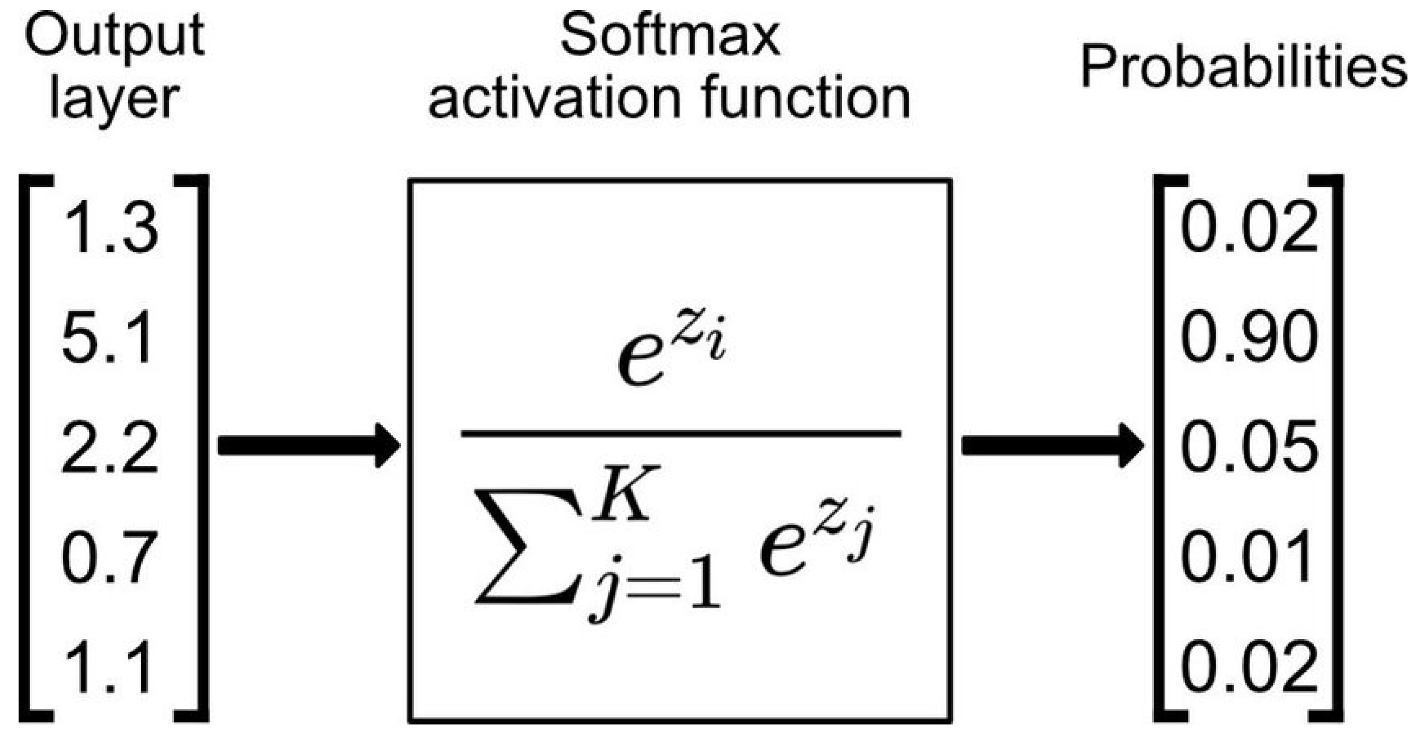
Let and , represent the SoftMax outputs for the classes "water" and "non-water" at each pixel location , where i and j denote the pixel coordinates in terms of width and height, respectively. The SoftMax function ensures that for any given pixel, the sum of these probabilities equals one, such that:
Let’s denote the pre- and post-flood scenarios as and . The difference between the post-flood and pre-flood predictions indicated as , is computed as:
A pixel is classified as "flooded" if ; otherwise, it is classified as "not flooded". This methodology ensures that the classification is based on a probabilistic approach, with the threshold value determining the sensitivity of flood detection. Rather than relying solely on absolute binary values of 0 and 1, this approach is expected to be more robust and can be tuned through a threshold, so that it can capture water pixels classified with lower probabilities.
6.5. Inference and Evaluation
The model’s performance in segmentation tasks is often evaluated using a variety of metrics, among which the Intersection Over Union (IoU), also known as the Jaccard Index, is the most used. This metric is particularly crucial because it provides a comprehensive measure of how accurately the predicted segmentation aligns with the ground truth. The IoU metric is defined as the ratio of the intersection area between the predicted segmentation and the ground truth to the union area of these two segments [33].
This equation quantifies the overlap between the predicted and actual segmentations. The values of IoU range from 0 to 1, where a higher value indicates a greater overlap and, consequently, a higher model accuracy. Unlike simple accuracy, which might be misleading especially in cases with class imbalance, IoU provides a more balanced and accurate evaluation of model performance.
The SAR model selection process is conducted through a k-fold cross-validation in the SAR-Optical dataset. To choose the best performing model, we utilize 5 fold cycles to train and test the model, allocating 70% for training and 30% for testing in each cycle. Each training cycle is trained for 100 epochs and we implement an early stopping mechanism set to stop when the model does not improve over 10 consecutive epochs. At this point, the model with the best performance is selected, to be tested on MMFlood-CD dataset.
The SAR model selection process is conducted through a k-fold cross-validation on the SAR-Optical dataset. Specifically, we employ 5-fold cycles to train and test the model, allocating 70% of the data for training and 30% for testing in each cycle. During each cycle, the model is trained for up to 100 epochs, with an early stopping mechanism in place to halt training if there is no improvement for 10 consecutive epochs. The model with the best performance is then selected for testing on the MMFlood-CD dataset.
6.6. MMFlood-CD Evaluation
In this phase, the SAR model’s predictions from the change detection module, applied to pre- and post-flood events, are compared with the EMS ground truth to evaluate performance. The process involves feeding the model two distinct images separately to generate pre- and post-flood predictions. These predictions are then processed by the change detection (CD) module to compute the differences between them. The Conditional Random Field (CRF) algorithm is then applied for post-processing refinement, to generate the final flood prediction. This prediction is visually compared with the EMS ground truth for performance assessment.
7. Experiments and Results
7.0.1. Implementation Details
Since GRD products have two-channel inputs (VV and VH) and because pre-trained models like ResNet require three-channel inputs, the GRD format is incompatible. Instead of converting them to RGB, which could lead to the loss of SAR-specific information, we modify the model forward function to add a zero-filled third channel at runtime and we train the ResNet model architectures from scratch.
To manage outliers effectively, SAR data is clipped to maintain values within a 0-1 range, and we further standardize this data to ensure a zero mean and unit variance, which is common practice before feeding the data into models. As for the loss function, we experimented both with the focal Tversky loss and the custom weighted cross-entropy function as explained in Section 6.2.1. The results have shown that the latter performs better. Our model adopts an Adam Optimizer with a learning rate of , a weight decay and momentum , which have shown to achieve a stable training after testing various parameters. To have a balance between generalization and memory limitations, we employed a batch size of 8. Our experiments employing different image patch sizes, ranging from 128 to 512, revealed that larger patches significantly enhance performance by capturing more spatial information. However, due to memory constraints, we settled on a consistent patch size of 512x512. Before feeding patches to the model, we use Albumentations [34] for random augmentations like flips (horizontal and vertical), rotations, and cropping. All with a probability of 0.5.
We tried two distinct settings for image processing. a) The first involves the generation of patches from the original images to ensure full coverage with minimal overlap, avoiding padding. Subsequently, we apply random augmentation. b) Alternatively, our second approach involves padding images to their maximum dimensions within the dataset, followed by random cropping of 512x512 patches from the original images, alongside the previously mentioned augmentations. The second technique, while slightly extending training time, improves model generalization.
7.0.2. Models benchmark results
Comparison with the Otsu thresholding baseline and different model combinations with encoders and decoders.
Figure 9.
Diagram to facilitate the understanding of the inference pipeline in the MMFlood-CD dataset.
Figure 9.
Diagram to facilitate the understanding of the inference pipeline in the MMFlood-CD dataset.
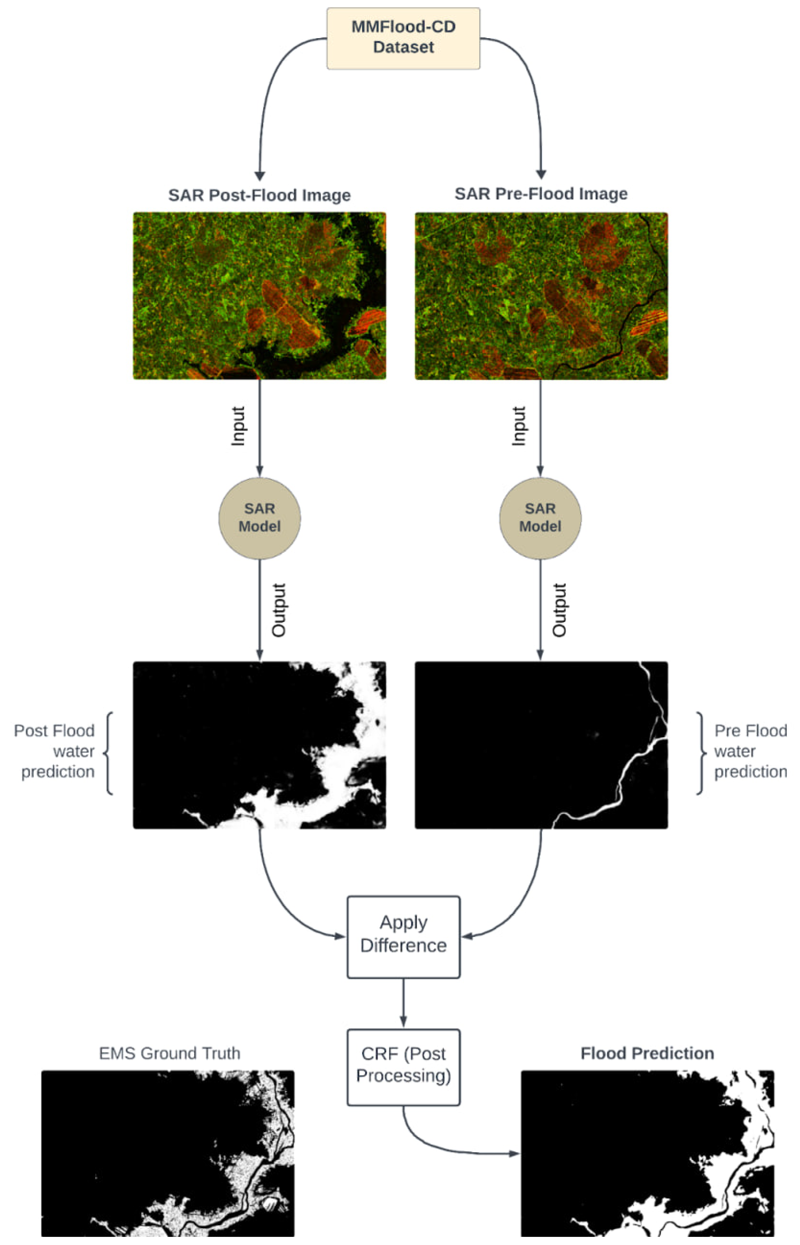
Table 2.
Model benchmark results
| Model Architecture | Accuracy | Recall | IoU |
| Otsu Thresholding | 0.78 ± 0.03 | 0.51 ± 0.02 | 0.27 ± 0.0 |
| Unet | 0.86 ± 0.03 | 0.82 ± 0.04 | 0.62 ± 0.01 |
| Unet + ResNet50 | 0.96 ± 0.02 | 0.95 ± 0.02 | 0.72 ± 0.02 |
| Unet + DenseNet201 | 0.85 ± 0.01 | 0.83 ± 0.01 | 0.63 ± 0.03 |
| Unet + VGG19 | 0.79 ± 0.05 | 0.78 ± 0.04 | 0.59 ± 0.03 |
7.1. Results on SAR-Optical Dataset
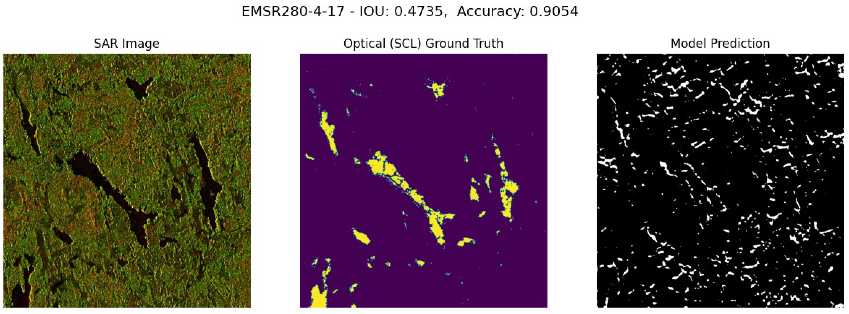
This section analyzes the performance of the top model, Unet + ResNet50, often surpassing the ground truth predictions from the Optical layer, used to train the model itself. During the EMSR442-0-6 flood event, despite cloud cover obscuring the Optical ground truth, the SAR model successfully identified the water regions. Additionally, the model excels in EMSR280-4-17 event by distinguishing snow-covered areas, which typically appear similar to water in SAR images. Here’s a detailed explanation of the labels in the images:
- SAR Image – The input SAR image.
- Optical (SCL) Ground Truth – Optical ground truth from Sentinel-2 SCL layer, provided by Copernicus.
- Model Prediction - The model prediction (presence of water, whether it’s due to flooding or permanent sources).
Figure 10.
Performance Analysis of EMSR258-13-1 Permanent Water in Albania.
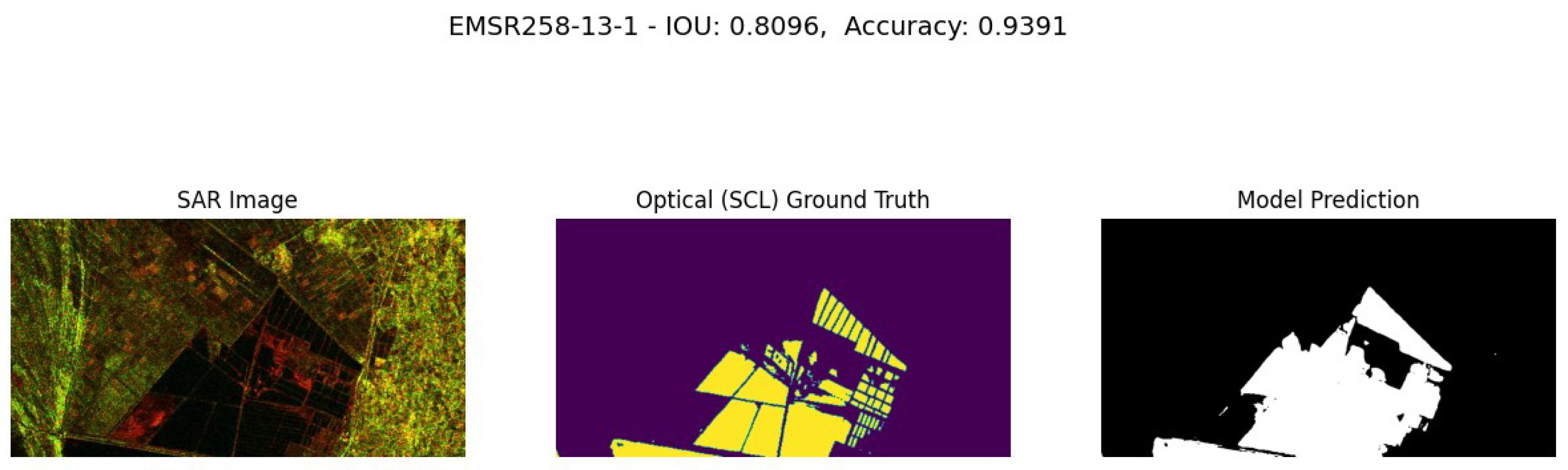
Figure 11.
Performance Analysis of EMSR407-1-4 Flood Event in the United Kingdom. Event Date: November 12, 2019 at 21:15.
Figure 11.
Performance Analysis of EMSR407-1-4 Flood Event in the United Kingdom. Event Date: November 12, 2019 at 21:15.
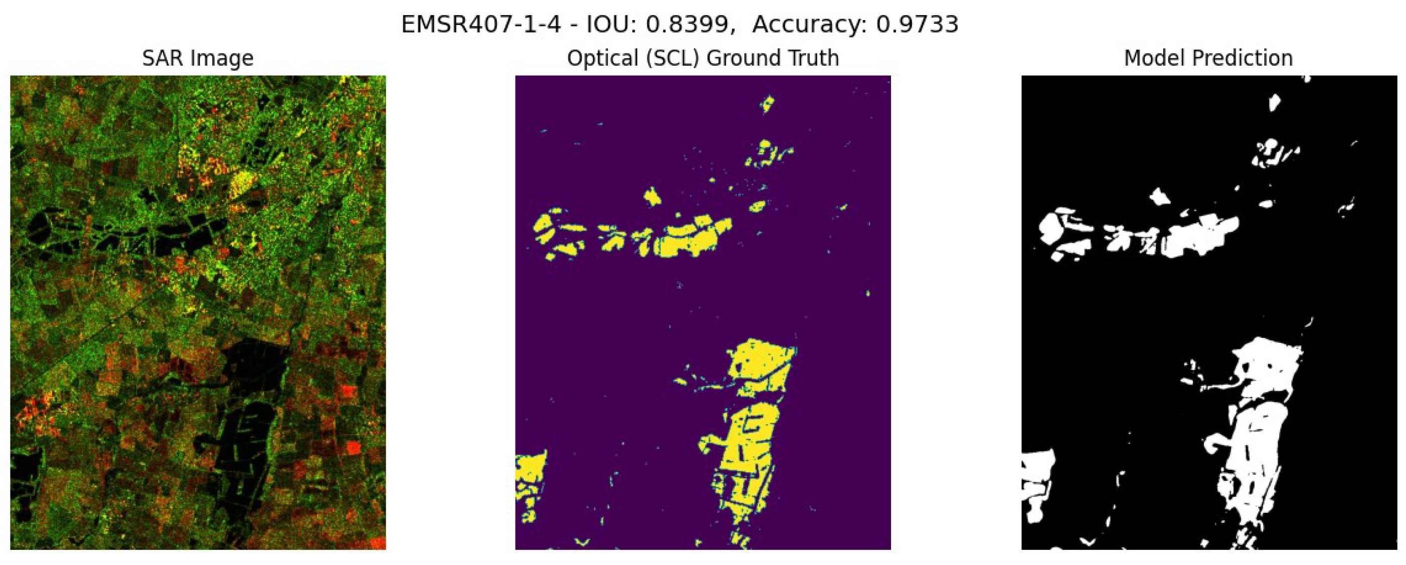
Figure 12.
Performance Analysis of EMSR277-2-0 Flood Event in Greece. Event Date: March 29, 2018 at 11:27.
Figure 12.
Performance Analysis of EMSR277-2-0 Flood Event in Greece. Event Date: March 29, 2018 at 11:27.
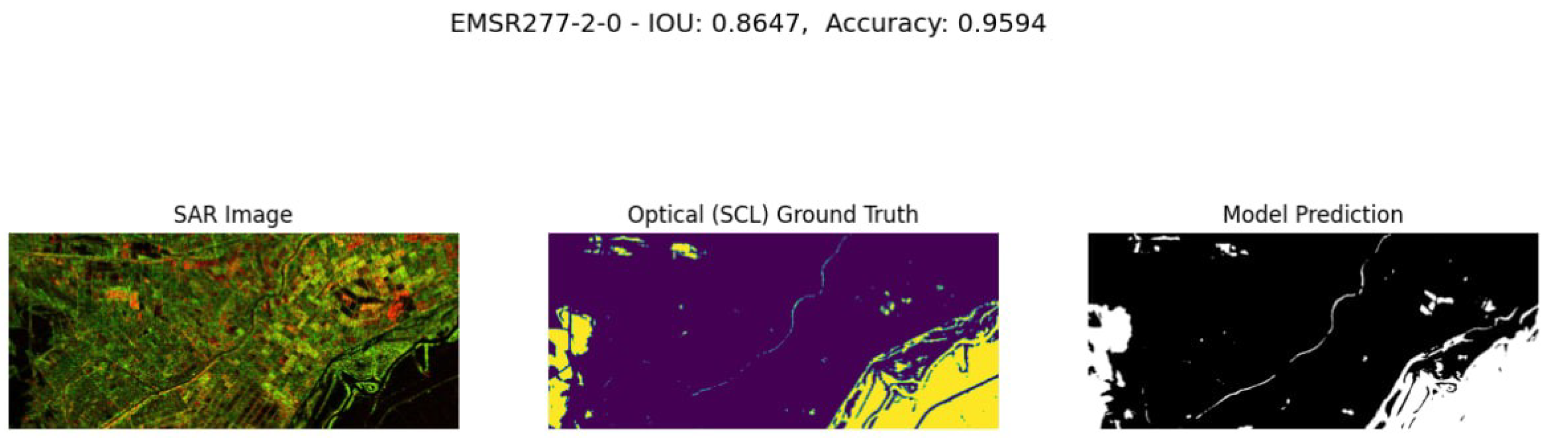
Figure 13.
Performance Analysis of EMSR501-0-3 Flood Event in Albania. Event Date: February 12, 2021 at 16:50.
Figure 13.
Performance Analysis of EMSR501-0-3 Flood Event in Albania. Event Date: February 12, 2021 at 16:50.
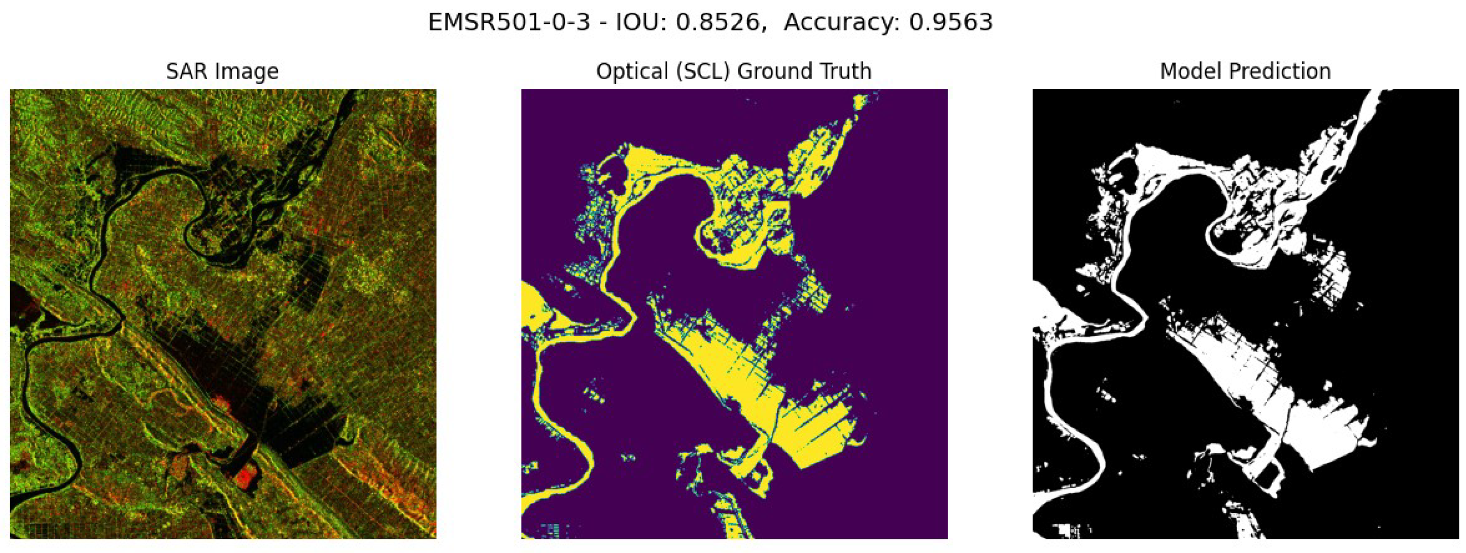
Figure 14.
Performance Analysis of EMSR442-0-6 Flood Event in Norway. Event Date: June 13, 2020 at 10:30.
Figure 14.
Performance Analysis of EMSR442-0-6 Flood Event in Norway. Event Date: June 13, 2020 at 10:30.
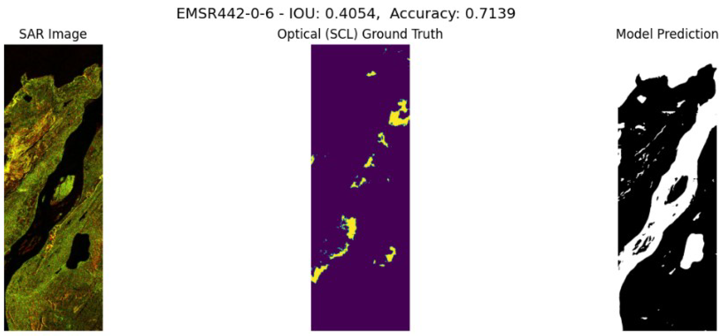
Figure 15.
Performance Analysis of EMSR280-4-17 Flood Event in Sweden. Event date: April 21, 2018 at 15:15.
Figure 15.
Performance Analysis of EMSR280-4-17 Flood Event in Sweden. Event date: April 21, 2018 at 15:15.
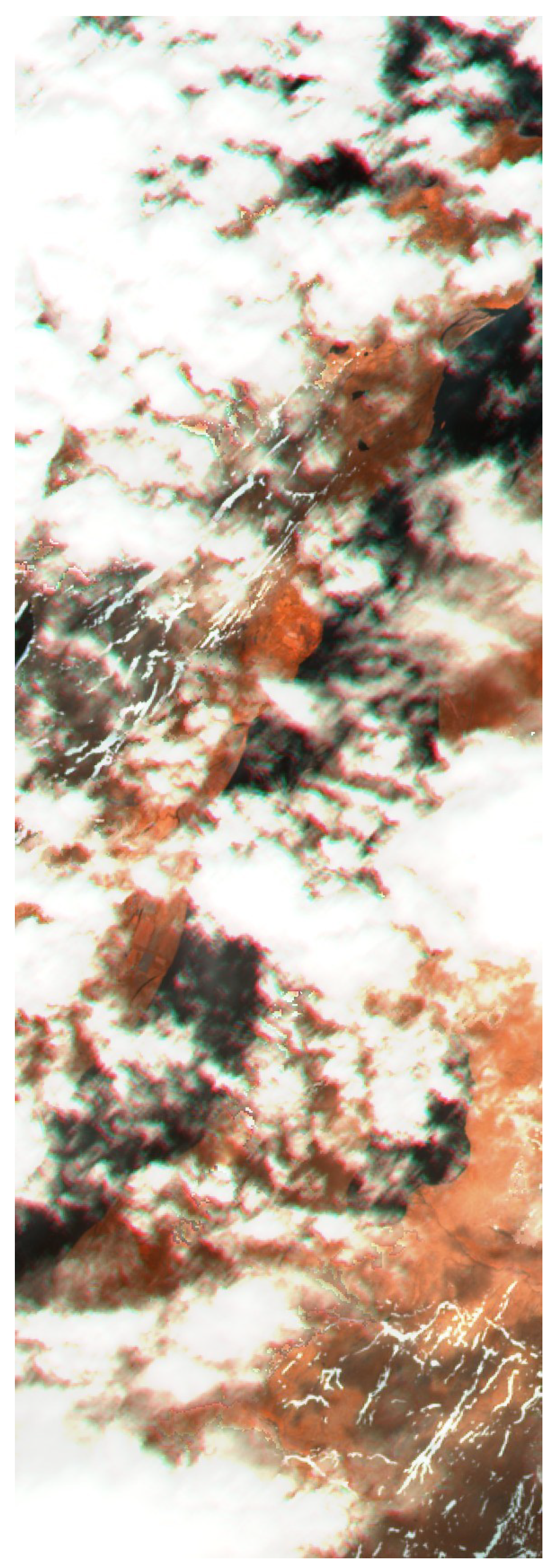
Overall, the model has demonstrated great performance. An example is shown in flood event EMSR442-0-6. Illustrated in Figure 14, this event highlights a section of water missing from the Optical (SCL) ground truth due to cloud cover obstruction. However, given SAR capacity of penetrating through clouds, the model was able to accurately detect those flood areas.
Figure 16.
RGB image of the EMSR442-0-6 flood event, from the Optical Sentinel-2 Satellite. It demonstrates the presence of cloud cover.
Figure 16.
RGB image of the EMSR442-0-6 flood event, from the Optical Sentinel-2 Satellite. It demonstrates the presence of cloud cover.
Another notable performance is seen in the flood event EMSR280-4-17. As illustrated in Figure 15, this event demonstrates the model’s capability to identify and exclude snow-covered areas. In SAR images, regions covered in snow closely resemble water, making them indistinguishable to the human eye. However, the model successfully distinguished these areas avoiding the misclassification of snow as water.
Figure 17.
RGB image of the EMSR280-4-17 flood event, from the Optical Sentinel-2 Satellite. It demonstrates the presence of snow
Figure 17.
RGB image of the EMSR280-4-17 flood event, from the Optical Sentinel-2 Satellite. It demonstrates the presence of snow
An example where the model underperforms the Optical, SCL ground truth, is given by the flood event in EMSR258-13-1. As shown in Figure 10, it’s evident that the model predictions are less accurate along the borders, likely due to the lower resolution of SAR resolution compared to the Optical ground truth.
7.2. Results on MMFlood-CD Dataset
In the following section is shown a visual comparison of the model prediction on flood events included in the MMFlood-CD dataset, using the trained model on SAR-Optical and the ground truth provided by EMS. Here’s a detailed explanation of the labels in the images:
- EMS Prediction - Ground Truth EMS to be compared against our model.
- SAR Model Prediction - The final flood prediction of our SAR Model.
- Pre-Flood Prediction - The pre-flood model predictions of water.
- Post-Flood Prediction- The post-flood model prediction of water.
- SAR Image Post-Flood - The SAR raw image post-flood.
- SAR Image Pre-Flood - The SAR raw image pre-flood.
Note that a lower IoU indicates that the EMS ground truth and the SAR-Optical Model predictions don’t closely match, either due to our SAR model or the EMS ground truth error.
Figure 18.
Comparative Analysis of the EMSR265-14-6 Flood Event in France. Event Date: January 23, 2018, at 19:17. Acquisition Date: January 25, 2018, at 05:59.
Figure 18.
Comparative Analysis of the EMSR265-14-6 Flood Event in France. Event Date: January 23, 2018, at 19:17. Acquisition Date: January 25, 2018, at 05:59.
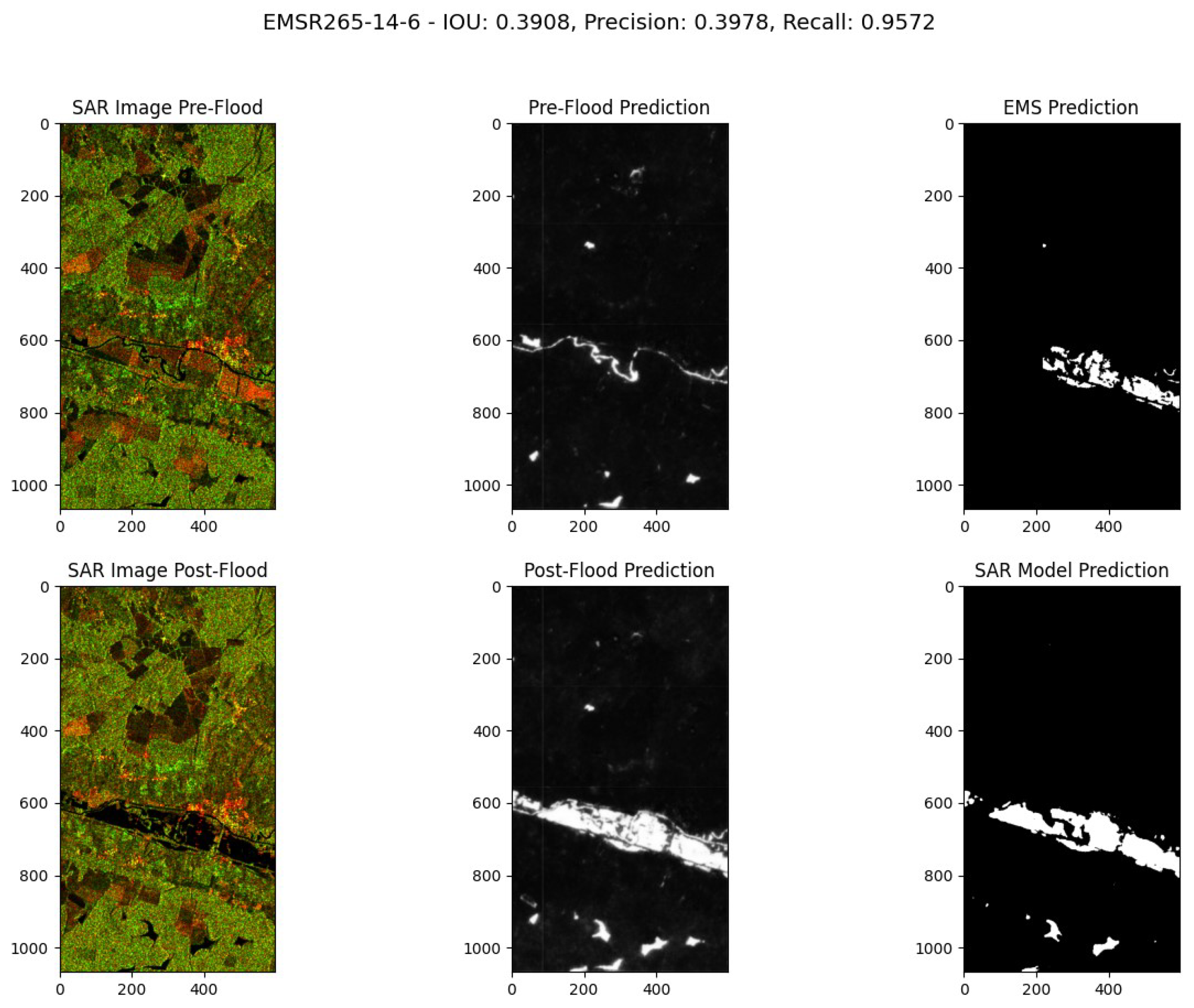
Figure 19.
Comparative Analysis of the EMSR332-2-1 Flood Event in Italy. Event Date: November 1, 2018, at 21:08. Acquisition Date: November 2, 2018 at 05:18.
Figure 19.
Comparative Analysis of the EMSR332-2-1 Flood Event in Italy. Event Date: November 1, 2018, at 21:08. Acquisition Date: November 2, 2018 at 05:18.
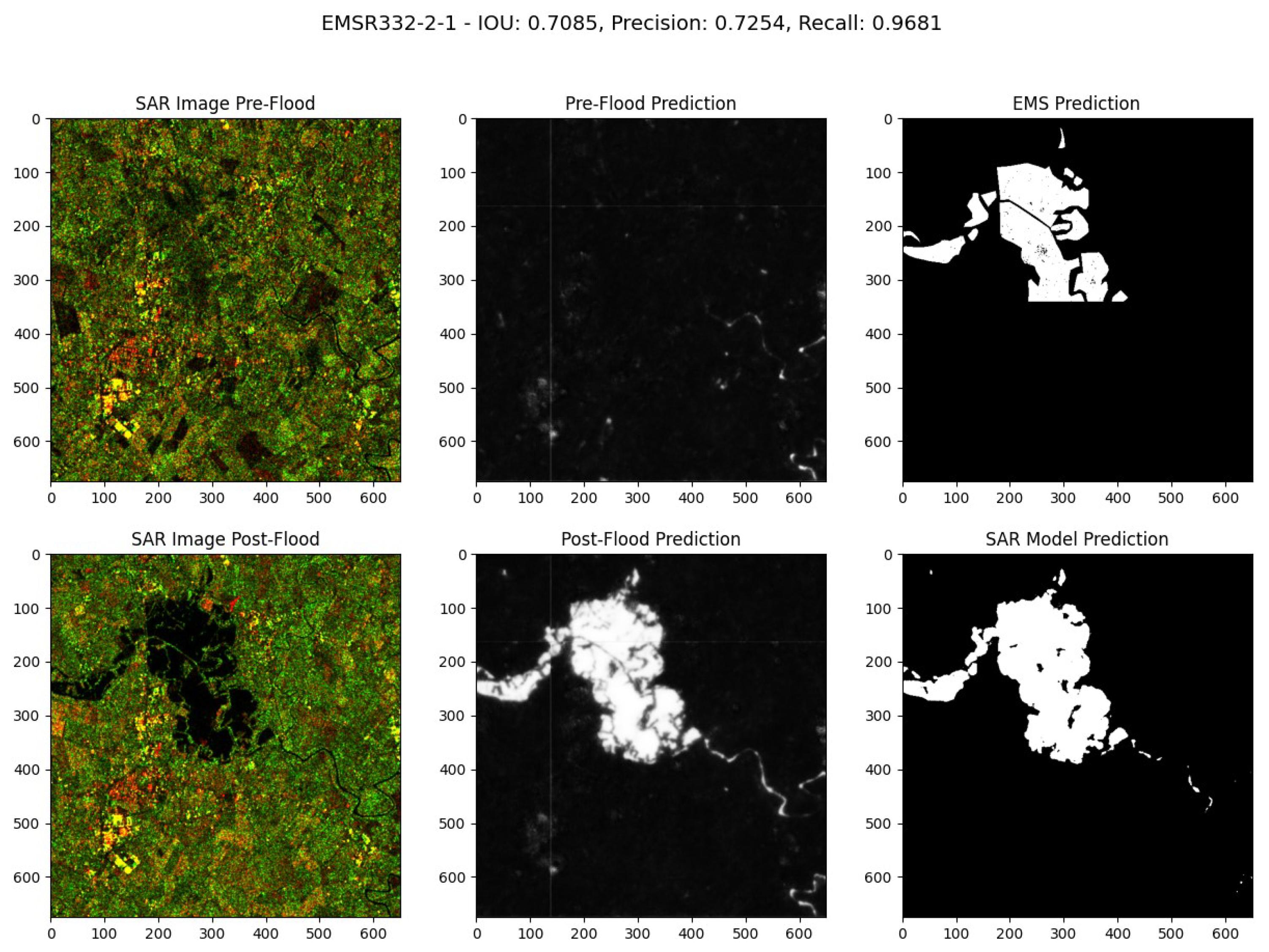
Figure 20.
Comparative Analysis of the EMSR314-2-2 Flood Event in Nigeria. Event Date: September 18, 2018, at 21:27. Acquisition Date: September 22, 2018 at 17:44.
Figure 20.
Comparative Analysis of the EMSR314-2-2 Flood Event in Nigeria. Event Date: September 18, 2018, at 21:27. Acquisition Date: September 22, 2018 at 17:44.
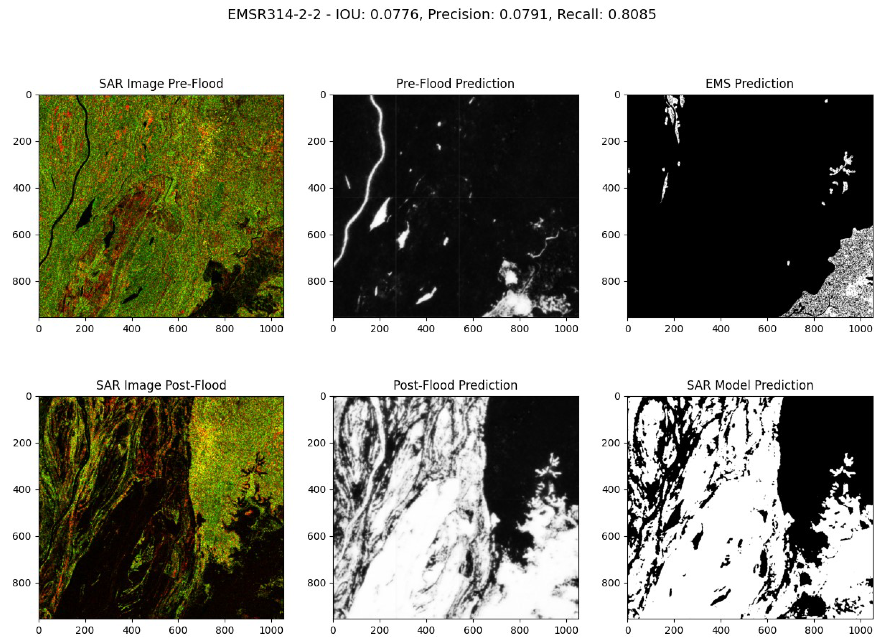
Figure 21.
Comparative Analysis of the EMSR-319-3-4 Flood Event in Tunisia. Event Date: September 29, 2018, at 17:42. Acquisition Date: October 3, 2018 at 17:11.
Figure 21.
Comparative Analysis of the EMSR-319-3-4 Flood Event in Tunisia. Event Date: September 29, 2018, at 17:42. Acquisition Date: October 3, 2018 at 17:11.
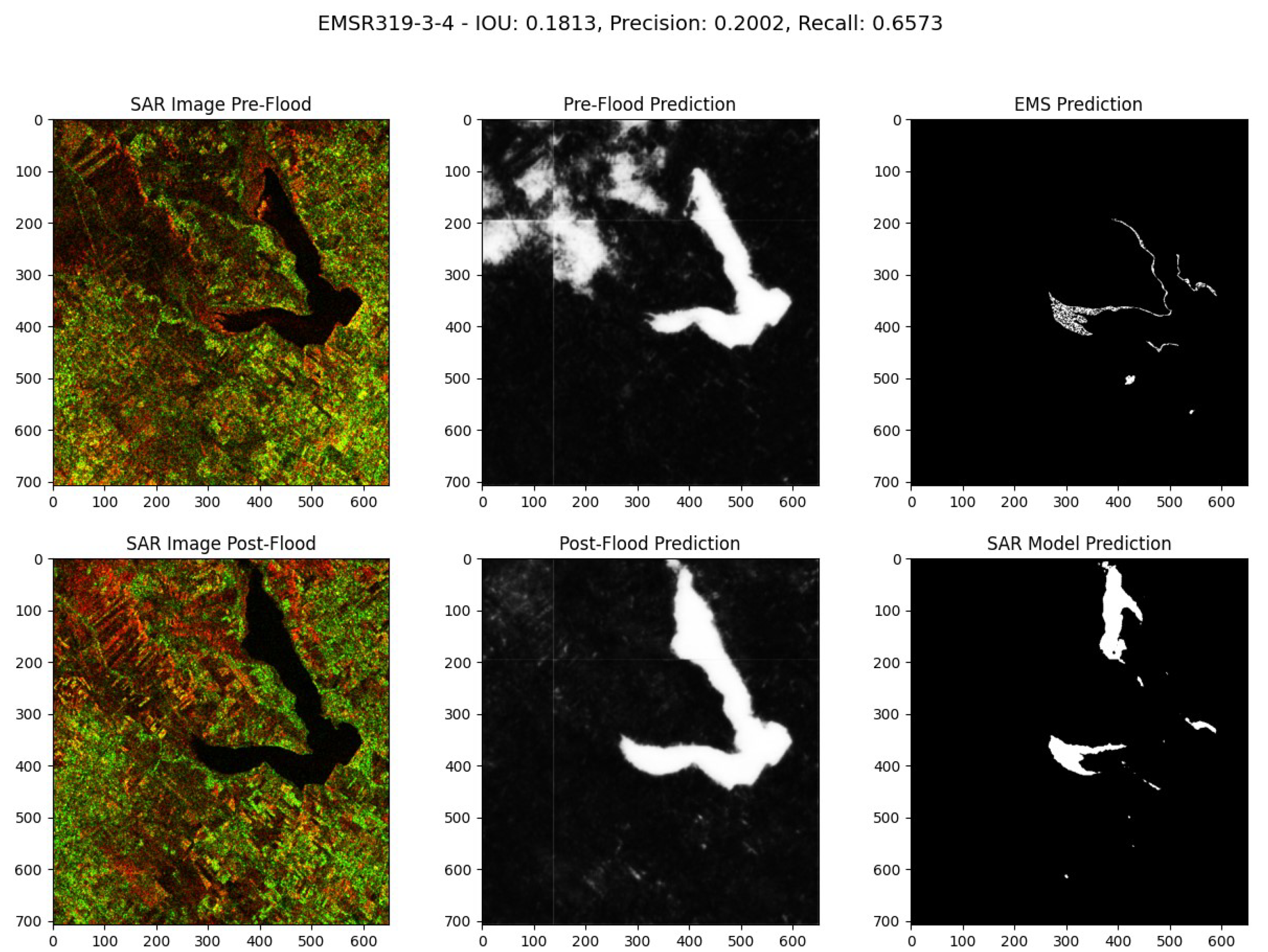
Figure 22.
Comparative Analysis of the EMSR-342-6-1 Flood Event in Australia. Event Date: February 1, 2019, at 04:45. Acquisition Date: February 5, 2019 at 19:43.
Figure 22.
Comparative Analysis of the EMSR-342-6-1 Flood Event in Australia. Event Date: February 1, 2019, at 04:45. Acquisition Date: February 5, 2019 at 19:43.
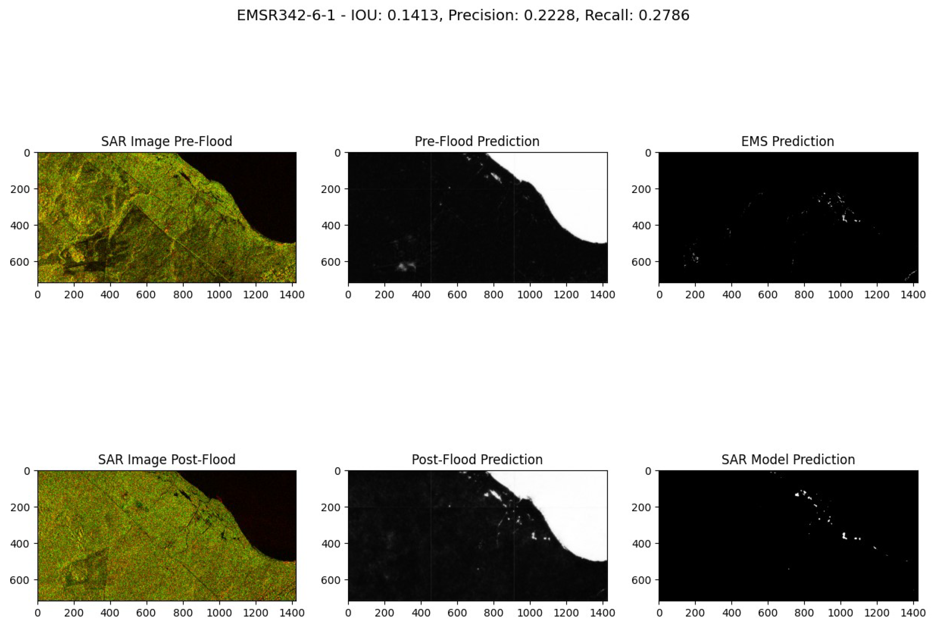
Figure 23.
Comparative Analysis of the EMSR-399-0-0 Flood Event in Vietnam. Event Date: October 28, 2019. Acquisition Date: October 28, 2019 at 22:45.
Figure 23.
Comparative Analysis of the EMSR-399-0-0 Flood Event in Vietnam. Event Date: October 28, 2019. Acquisition Date: October 28, 2019 at 22:45.
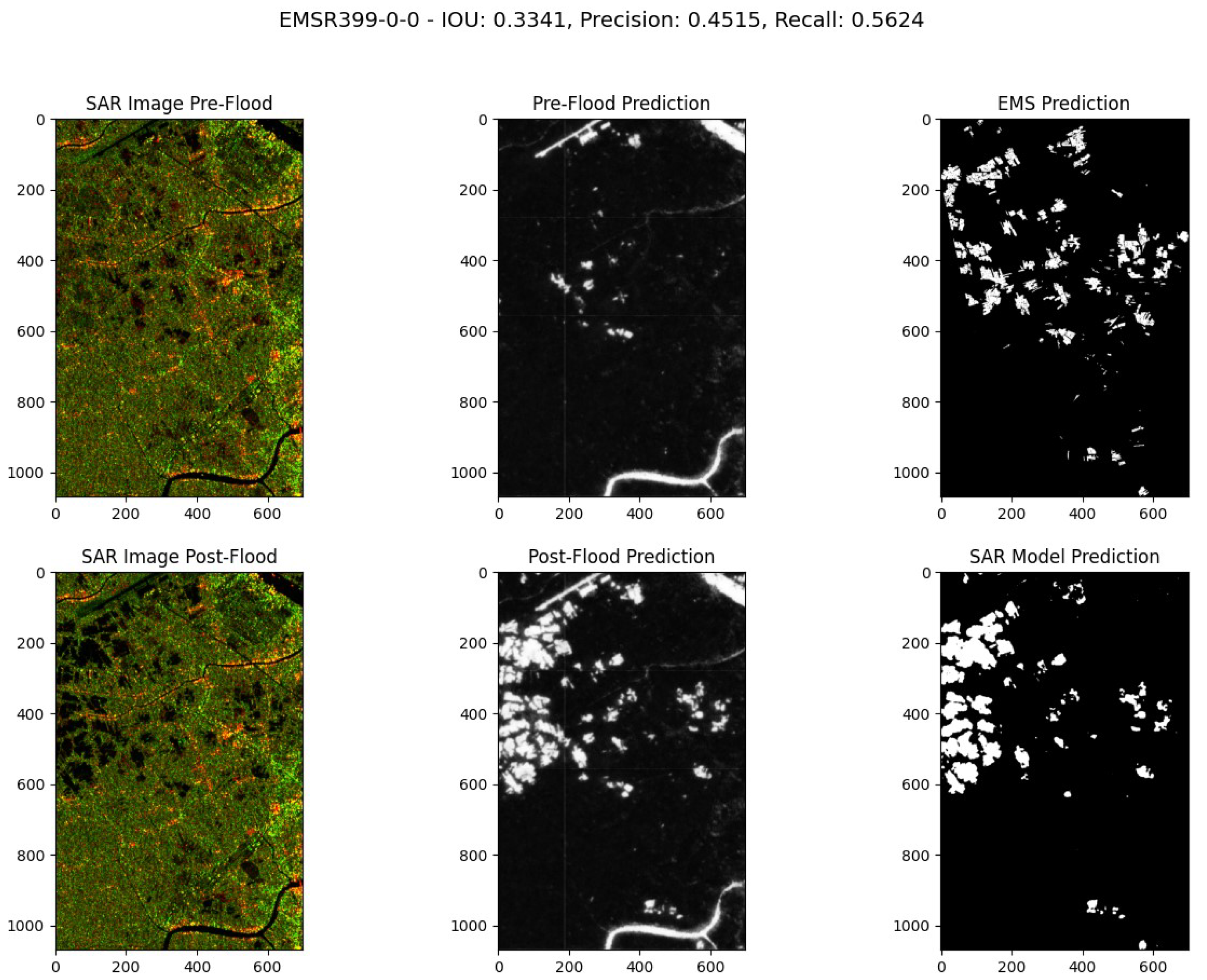
The model has demonstrated great performance in this qualitative evaluation. Despite the inability to directly compare its performance with an alternative ground truth, we can easily discern areas where the EMS model might fail by examining both pre- and post-flood SAR images. Figure 18, Figure 19, and Figure 21 are possible examples where the EMS model may have misses certain flood areas, detecting them only partially compared to our model. In Figure 20, EMS model appears to miss a rapid flood event that our model correctly detects. Figure 21 is the only instance where both the EMS and our SAR model produce matching predictions.
8. Conclusions
In summary, the project introduces a novel framework that aims to improve flood mapping using Synthetic Aperture Radar (SAR) and Multi-Spectral Imaging (MSI). By leveraging the precision of MSI and the all-weather capabilities of SAR, a transfer-learning framework is developed to improve the SAR model flood mapping accuracy. Through transfer learning, the SAR model (“student”) is trained using Optical/MSI models (“teacher”), achieving a remarkable flood mapping performance, with an Intersection Over Union (IoU) score of 0.72. We rigorously evaluate the model’s precision and reliability against traditional methods and qualitatively compare it with ground truth data provided by Emergency Management Services (EMS). The promising results of the model reaching an IoU score of 0.72 and its capacity to adapt in identifying floods under cloud cover and snow, demonstrate its ability at detecting flood.
Although the model surpasses existing solutions, there is room for improvement. Future work could be focused on expanding the dataset, refining data collection methods, and exploring different augmentations to potentially enhance the quality of data and labels. Furthermore, the exploration of alternate architectures, and a deeper hyper-parameter optimization could improve the model performance.
Funding
This research received no external funding and the APC was funded by University Of Stirling.
Conflicts of Interest
The authors declare no conflicts of interest.
References
- On the Assessment and Management of Flood Risks (Text with EEA relevance), 2007. Available: https://eur-lex.europa.eu/legal-content/EN/TXT/PDF/?uri=CELEX:32007L0060&from=EN.
- Lendering, K.T.; Jonkman, S.N.; Kok, M. Effectiveness of Emergency Measures for Flood Prevention. Journal of Flood Risk Management 2015, 9, 320–334. [Google Scholar] [CrossRef]
- Tsokas, A.; Rysz, M.; Pardalos, P.M.; Dipple, K. SAR data applications in earth observation: An overview. Expert Systems with Applications 2022, 205, p–117342. [Google Scholar] [CrossRef]
- Shao, Y. Effect of dielectric properties of moist salinized soils on backscattering coefficients extracted from RADARSAT image. IEEE, 2003. Available: https://ieeexplore.ieee.org/abstract/document/1221799.
- Amitrano, D.; Di Martino, G. Unsupervised Rapid Flood Mapping Using Sentinel-1 GRD SAR Images. IEEE Journals & Magazine, 2018. Available: https://ieeexplore.ieee.org/abstract/document/8291019.
- de, W. et al. Analysis of Environmental and Atmospheric Influences in the Use of SAR and Optical Imagery from Sentinel-1, Landsat-8, and Sentinel-2 in the Operational Monitoring of Reservoir Water Level. Remote Sensing 2022, 14, 2218–2218. [Google Scholar] [CrossRef]
- Schumann, G.; Di Baldassarre, G.; Alsdorf, D.; Bates, P.D. Near real-time flood wave approximation on large rivers from space: Application to the River Po, Italy. Water Resources Research 2010, 46. [Google Scholar] [CrossRef]
- Bentivoglio, R.; Isufi, E.; Jonkman, S.N.; Taormina, R. Deep learning methods for flood mapping: a review of existing applications and future research directions. Hydrology and Earth System Sciences 2022, 26, 4345–4378. [Google Scholar] [CrossRef]
- Qiu, J.; Cao, B.; Park, E.; Yang, X.; Zhang, W.; Tarolli, P. Flood Monitoring in Rural Areas of the Pearl River Basin (China) Using Sentinel-1 SAR. Remote Sensing 2021, 13, 1384. [Google Scholar] [CrossRef]
- Liang, J.; Liu, D. A local thresholding approach to flood water delineation using Sentinel-1 SAR imagery. ISPRS Journal of Photogrammetry and Remote Sensing 2020, 159, 53–62. [Google Scholar] [CrossRef]
- Chini, M. A Hierarchical Split-Based Approach for Parametric Thresholding of SAR Images: Flood Inundation as a Test Case. IEEE, 2017. Available: https://ieeexplore.ieee.org/document/8017436.
- Amitrano, D.; Di Martino, G.; Di Simone, A.; Imperatore, P. Flood Detection with SAR: A Review of Techniques and Datasets. Remote Sensing 2024, 16. [Google Scholar] [CrossRef]
- Sarker, C.; Mejias, L.; Maire, F.; Woodley, A. Flood Mapping with Convolutional Neural Networks Using Spatio-Contextual Pixel Information. Remote Sensing 2019, 11, 2331. [Google Scholar] [CrossRef]
- Syahdani, F.A. Implementasi Convolutional Neural Network Dalam Mendeteksi Cuaca Dari Foto. Master’s Thesis, Universitas Multimedia Nusantara, 2023. Available: https://kc.umn.ac.id/id/eprint/23969/4/BAB_II.pdf.
- Long, J.; Shelhamer, E.; Darrell, T. Fully Convolutional Networks for Semantic Segmentation. 2015. Available: https://arxiv.org/pdf/1411.4038.pdf.
- Nemni, E.; Bullock, J.; Belabbes, S.; Bromley, L. Fully Convolutional Neural Network for Rapid Flood Segmentation in Synthetic Aperture Radar Imagery. Remote Sensing 2020, 12, 2532. [Google Scholar] [CrossRef]
- Oliveira, H.; Silva, G.; Machado, K.; Nogueira, K.; Santos. Fully Convolutional Open Set Segmentation. Machine Learning 2021, 112, 1733–1784. [Google Scholar] [CrossRef]
- Ronneberger, O.; Fischer, P.; Brox, T. U-Net: Convolutional Networks for Biomedical Image Segmentation. arXiv.org 18 May 2015. Available: https://arxiv.org/abs/1505.04597.
- He, K.; Zhang, X.; Ren, S.; Sun, J. Deep Residual Learning for Image Recognition. arXiv.org, 10 December 2015. Available: https://arxiv.org/abs/1512.03385.
- Chu, Z. Sea-Land Segmentation With Res-UNet And Fully Connected CRF. In IEEE Conference Publication, IEEE Xplore, 1 January 2019. Available online: https://ieeexplore.ieee.org/document/8900625 (accessed on 26 February 2024).
- Lafferty, J.; McCallum, A.; Pereira, F. Conditional Random Fields: Probabilistic Models for Segmenting and Labeling Sequence Data. January 2001. Available: http://www.cs.columbia.edu/~jebara/6772/papers/crf.pdf. (accessed on 26 February 2024).
- Krähenbühl, P.; Koltun, V. Efficient Inference in Fully Connected CRFs with Gaussian Edge Potentials. arXiv.org, 20 October 2012. Available: https://arxiv.org/abs/1210.5644.
- Yadav, R.; Nascetti, A.; Azizpour, H.; Ban, Y. Unsupervised Flood Detection on SAR Time Series Using Variational Autoencoder. International Journal of Applied Earth Observation and Geoinformation 2024, 126, 103635. [Google Scholar] [CrossRef]
- Bonafilia, D.; Tellman, B.; Anderson, T.; Issenberg, E. Sen1Floods11: A Georeferenced Dataset to Train and Test Deep Learning Flood Algorithms for Sentinel-1. openaccess.thecvf.com, 2020. Available: https://openaccess.thecvf.com/content_CVPRW_2020/html/w11/Bonafilia_Sen1Floods11_A_Georeferenced_Dataset_to_Train_and_Test_Deep_Learning_CVPRW_2020_paper.html (accessed on 28 October 2021).
- MMFlood: A Multimodal Dataset for Flood Delineation From Satellite Imagery. Available online: https://ieeexplore.ieee.org/document/9882096 (accessed on 19 February 2024).
- Paul, S.; Carted, S. ; Ganju. Flood Segmentation on Sentinel-1 SAR Imagery with Semi-Supervised Learning. Accessed: 27 February 2024. Available: https://arxiv.org/pdf/2107.08369.pdf.
- Peña, F.J.; Hübinger, C.; Payberah, A.H.; Jaramillo, F. DeepAqua: Semantic Segmentation of Wetland Water Surfaces with SAR Imagery Using Deep Neural Networks Without Manually Annotated Data. International Journal of Applied Earth Observation and Geoinformation 2024, 126, 103624. [Google Scholar] [CrossRef]
- Main-Knorn, M.; Pflug, B.; Louis, J.; Debaecker, V.; Müller-Wilm, U.; Gascon, F. Sen2Cor for Sentinel-2. Image and Signal Processing for Remote Sensing XXIII, 2017. [Google Scholar] [CrossRef]
- Filipponi, F. Sentinel-1 GRD Preprocessing Workflow. In Proceedings of the Proceedings, vol. 18, no. 1, p. 11, June 2019. [CrossRef]
- A Novel Focal Tversky Loss Function With Improved Attention U-Net for Lesion Segmentation. In IEEE Conference Publication, IEEE Xplore. Available online: https://ieeexplore.ieee.org/document/8759329 (accessed on 1 March 2024).
- Bai, Y. et al. Enhancement of Detecting Permanent Water and Temporary Water in Flood Disasters by Fusing Sentinel-1 and Sentinel-2 Imagery Using Deep Learning Algorithms: Demonstration of Sen1Floods11 Benchmark Datasets. Remote Sensing 2021, 13, 2220. [Google Scholar] [CrossRef]
- Ioffe, S.; Szegedy, C. Batch Normalization: Accelerating Deep Network Training by Reducing Internal Covariate Shift. arXiv.org, 2015. Available: https://arxiv.org/abs/1502.03167.
- Rezatofighi, H.; Tsoi, N.; Gwak, J.; Sadeghian, A.; Reid, I.; Savarese, S. Generalized Intersection Over Union: A Metric and a Loss for Bounding Box Regression. Thecvf.com, 2019, pp. 658–666. Available: https://openaccess.thecvf.com/content_CVPR_2019/html/Rezatofighi_Generalized_Intersection_Over_Union_A_Metric_and_a_Loss_for_CVPR_2019_paper.html.
- Buslaev, A.; Iglovikov, V.I.; Khvedchenya, E.; Parinov, A.; Druzhinin, M.; Kalinin, A.A. Albumentations: Fast and Flexible Image Augmentations. Information 2020, 11, 125. [Google Scholar] [CrossRef]
Disclaimer/Publisher’s Note: The statements, opinions and data contained in all publications are solely those of the individual author(s) and contributor(s) and not of MDPI and/or the editor(s). MDPI and/or the editor(s) disclaim responsibility for any injury to people or property resulting from any ideas, methods, instructions or products referred to in the content. |
© 2024 by the authors. Licensee MDPI, Basel, Switzerland. This article is an open access article distributed under the terms and conditions of the Creative Commons Attribution (CC BY) license (http://creativecommons.org/licenses/by/4.0/).
Copyright: This open access article is published under a Creative Commons CC BY 4.0 license, which permit the free download, distribution, and reuse, provided that the author and preprint are cited in any reuse.
Submitted:
21 June 2024
Posted:
21 June 2024
Read the latest preprint version here
Alerts
This version is not peer-reviewed
Submitted:
21 June 2024
Posted:
21 June 2024
Read the latest preprint version here
Alerts
Abstract
Our world is increasingly challenged by managing the impacts of natural disasters, particularly floods, which are frequent, dangerous, and costly. Traditional flood mapping methods, reliant on Optical satellites (MSI), struggle under cloud cover which is typical during such events. Synthetic Aperture Radar (SAR) offers a promising alternative with its cloud-penetrating capability, though its use has been limited due to complexity and data labeling challenges. This project aims to develop a SAR-based flood segmentation model that can rapidly and accurately map floods globally, with high adaptability to different flood types and regions. By utilizing deep learning and a novel transfer-learning technique that combines the strengths of Optical/MSI and SAR data, the model seeks to bypass the challenges of manual labeling and improve mapping accuracy. Initial results show the model's effective generalization across various flood events, with superior performance indicated by an Intersection over Union (IoU) of 0.72, outperforming existing methods and demonstrating promising capabilities in precise flood mapping.
Keywords:
Subject: Computer Science and Mathematics - Artificial Intelligence and Machine Learning
1. Introduction
Floods are increasingly threatening due to climate change, posing significant risks to lives, property, and infrastructure [1]. Effective flood mapping, crucial for disaster response, necessitates rapid and precise techniques. Preventive and emergency measures are essential for mitigating flood impacts [2]. Satellite data, particularly from Multi-Spectral Imaging (MSI) and Synthetic Aperture Radar (SAR), play a key role in near real-time flood mapping, aiding effective decision-making. While MSI usability is limited by cloud cover, SAR can penetrate clouds, providing reliable data even in adverse weather conditions. When it comes to Deep Learning, the application of SAR in flood mapping remains limited due to data scarcity and high costs of manual labelling. Our project aims at developing an automated, reliable flood mapping model using SAR, enhanced by MSI through an innovative transfer-learning approach. This model seeks to deliver accurate flood maps across multiple regions and under various conditions to improve disaster response capabilities.
In recent years, Synthetic Aperture Radar (SAR) polarimetric data has been a valuable tool in the field of flood mapping due to its unique capabilities and advantages. SAR operates by emitting radar signals towards the Earth’s surface and measuring the return signals (process known as backscattering) [3]. While traditional optical sensors, using visible light, can be interpreted by human eyes, SAR requires a different mindset. Objects on the Earth’s surface scatter the radar signals in different ways based on the object’s dimension, shape and material, allowing to differentiate various types of terrain and objects [3]. Water, with its high dielectric constant, tends to scatter all incoming radiation in a specular direction [4] when the surface is flat. This typically results in very low backscattering signals from such areas, a characteristic that is particularly useful for mapping floodwaters over non-flooded areas using SAR intensity images. In our project we will make use of the ESA Sentinel-1 constellation from Copernicus, which is an European Union program aimed at monitoring the Earth. Our focus will primarily be on the intensity features of the imagery, for which we will exclusively use the Ground Range Detected (GRD) products from the Sentinel-1 mission. GRD products are pre-processed images which are lighter and do not include phase information, but they retain the intensity feature, which is crucial for differentiating between water and land surfaces [5]. Historically, most SAR applications for flood segmentation have been using statistical thresholding to discriminate between water and non-water pixels [6,7]. Only recently, with the advance in Machine Learning (ML), new models are increasingly being adopted [8]. Among these, Convolutional Neural Networks (CNNs) are particularly prominent for image recognition tasks, offering significant improvements over traditional threshold-based methods for flood segmentation. Unlike threshold approaches that rely on individual pixels, CNNs consider the context provided by neighboring pixels. We will explore the details of these advancements in the subsequent sections.
2. Thresholding
Numerous flood models in the literature have been using thresholding techniques like Otsu thresholding [9] to differentiate water from land surface, which in contrast has an higher backscatter signal; Otsu thresholding in simple terms, finds the best thresholding value to separate the two distributions. However, this is not always possible, in fact in some cases, the two distributions are indistinguishable and are mixed in one single bell curve; in such cases the Otsu method fails to detect the optimal threshold. Many approaches try to solve this problem by applying local thresholding techniques [10]; in [11] an iterative algorithm searches for tiles of variable sizes to find a local threshold that can better distinguish the distributions of the two classes. These methodologies have been widely used, but they struggle in challenging areas where the backscatter values resemble those of water such as asphalt, dry regions, radar shadows, or ice and snow, which in turns gives many false positives [12]. To account for the cases where the thresholding approaches fail, recent approaches exploit spatial information of adjacent pixels [13]. In SAR images, neighbours pixels often exhibit similar values, the spatial information refers to the information that can be gathered by exploiting adjacent pixels to distinguish structure, texture, and features present in the image. In the next section we will delve into deep learning models and see how they can exploit the spatial information to better delineate flood areas.
3. Deep Neural Networks
Deep learning models have become more and more popular nowadays and are constantly evolving. They are also increasingly being applied in recent research, including for tasks such as flood segmentation. Notably [8] does an overview of existing deep learning methods for flood segmentation, and it suggests the preference towards specific model architectures based on their “inductive biases”. The inductive bias refers to the set of assumptions a learning algorithm makes or is expected to make to predict outputs (labels) based on inputs (features). Based on the assumption that in flood analysis, SAR data often exhibit spatial correlations between adjacent pixels, NN (Neuronal Network) layers can be configured to exploit these data structures, by introducing constraints on the connections and interactions between inputs and outputs and favouring certain model architectures over others [8]. One way to exploit spatial information is the use of a convolutional layer, which is the core component of Convolutional Neural Network (CNN).
3.1. CNN (Convolutional Neural Network)
Convolutional Neural Networks (CNNs) are a type of model in the field of deep learning, particularly useful at processing data with a grid shape, such as images. Central to CNNs are convolutional layers, which exploit spatial information by capturing the local relationships among pixels through the use of filters. In a convolutional layer, traditional neuron weights are replaced with filters. These filters compute new values for each pixel by considering the local relationships with its neighbors. The architecture is designed to progressively abstract higher-level features from the raw input in the initial layers to more abstract representations in deeper layers, making CNNs particularly powerful for tasks like image classification.
Figure 1.
Illustration of the convolutional operation, visualized through a 3x3 kernel applied to an input image, that produces a feature map highlighting detected patterns. This process, core of CNNs, enables the network’s to automatically learn spatial relationships of features [14].
Figure 1.
Illustration of the convolutional operation, visualized through a 3x3 kernel applied to an input image, that produces a feature map highlighting detected patterns. This process, core of CNNs, enables the network’s to automatically learn spatial relationships of features [14].
3.2. Segmentation Models: An Overview
The standard CNN architecture can’t be directly used for image segmentation. In fact, as shown in Figure 2 the fully connected layers link the pooling layers to a 1D output, which loses spatial context. To retain the spatial context in the output layer, other segmentation specific architectures have been proposed in the literature. The Fully Convolutional Network (FCN) introduced in [15] utilizes pre-existing CNN architectures designed for classification tasks (such as AlexNet, VGG, etc.). These architectures are adapted into fully convolutional networks and their learned representations are transferred to the segmentation task through fine-tuning. FCNs introduced the idea of replacing fully connected layers with convolutional layers, to produce pixel-wise predictions for segmentation. The architecture consists of an encoder path, which downsamples the input image to extract features, and a decoder path, which upsamples the features to produce the segmentation map. FCNs have been effectively applied in tasks such as flood segmentation, as demonstrated in [16].
Figure 2.
Abstract view of a CNN architecture for classification tasks. Following convolutional and pooling layers, the network typically ends with fully connected layers that integrate these learned features into predictions or classifications, outputting a one-dimensional array corresponding to the classes [14].
Figure 2.
Abstract view of a CNN architecture for classification tasks. Following convolutional and pooling layers, the network typically ends with fully connected layers that integrate these learned features into predictions or classifications, outputting a one-dimensional array corresponding to the classes [14].
Figure 3.
Architecture example of a CNN for image classification and its equivalent FCN architecture with the same backbone for semantic segmentation. KKCs = 4 refers to the number of output classes (channels) probabilities for pixel wise predictions. We can see that in the FCN, the fully connected layers are replaced by convolutions to produce pixel-wise predictions [17].
In 2015, a novel paper [18] proposed the U-Net architecture which builds upon the ideas introduced by FCNs but adds the concept of skip connections. The idea behind it is that each encoder and decoder layer is symmetrically linked with a skip connection, that is achieved by concatenating the output from encoding layers to corresponding decoding layers. The goal was to provide a more detailed segmentation mask by exploiting global and local features of an image. This concept, initially proposed in [18], was further reproposed a few months later by a new model architecture called ResNet (Residual Nets) [19]. ResNet builds upon the concept of skip connections from Unet [18] but approaches it from a different angle. ResNet [19] solves a common issue encountered in deep neural networks: as the network gets deeper with more layers, the gradient (used to update the weights based on the error) diminishes significantly during backpropagation, leading to difficulties in updating the weights of earlier layers. This is known as the gradient vanishing problem. Recent advances in segmentation combine the power of ResNet deep features extraction into the Unet Encoder, which significantly improve the segmentation performance. This hybrid architecture has been applied for sea-land optical segmentation in [20], demonstrating that replacing ResNet into the Unet architecture significantly improves feature representation. This enhancement, together with fully connected Conditional Random Fields (CRFs) as post-processing predictions refinement, leads to more accurate delineation of coastlines and better-preserved regions in sea-land segmentation tasks as shown in [20].
3.3. Conditional Random Fields (CRFs) in Segmentation
Conditional Random Fields (CRFs) have been widely used as a post-processing technique to refine segmentation results. Initially developed as a probabilistic framework for segmenting and labelling sequential data [21], CRFs were later adapted into fully connected CRFs to address the challenges of semantic segmentation. However, the widespread adoption of fully connected CRFs was slowed down by the computational demands of their inference processes. The scenario changed with the introduction of an efficient inference algorithm shown in [22], making fully connected CRFs more efficient and viable for practical use especially as a common technique for post-processing in segmentation tasks. By modelling the spatial dependencies between pixels, CRFs improve the coherence and accuracy of the segmentation output, particularly in distinguishing between closely related classes and preserving boundary definitions. Their application, combined with advanced neural network architectures like U-Net and ResNet, represents a comprehensive approach to tackling complex segmentation tasks with improved precision. Notably in [20], it is demonstrated that the use of CRF as a post-processing stage enhances the segmentation predictions results. In our research, we adopt the U-Net architecture integrated with an encoder block derived from the ResNet encoder. Furthermore, our exploration will include the application of CRFs, in alignment with current trends indicated in the literature.
4. Unsupervised Models for Flood Segmentation
The complexity and cost of data retrieval, preprocessing, and manual labeling make building a new dataset from scratch difficult, emphasizing the need for unsupervised approaches. To address these current dataset limitations, several papers have proposed self-supervised or fully unsupervised techniques for flood segmentation. These approaches eliminate the need for manually labeled datasets, which are expensive, labor-intensive and not always accurate.
4.1. Fully Unsupervised Learning
CLVAE [23] proposed an unsupervised model based on change detection to detect floods, which is reported to achieve an Intersection Over Union (IoU) of 64.53%. Their architecture is composed of a Variational Autoencoder (VAE) with a Contrastive Learning loss to automatically extract and learn latent distributions from images. The model is trained on mixed patches of floods from Sen1Floods11 [24] and MMFlood [25] dataset. Their approach is to apply a VAE model to both pre- and post-flood images, and compute the difference on their latent distributions. Then, based on a manually selected threshold, the flood over non-flood pixels are classified. Although this approach solves the need for labels, it comes with some limitations. The VAE architecture is traditionally designed to extract latent distributions of entire images, presenting challenges when applied for pixel-level segmentation tasks. Since it’s unpractical to apply the VAE model to single pixels, their proposed solution involves utilizing extremely small patch sizes of 16x16 so that the classification is conducted in these entire blocks of 16x16 pixels. This approach inevitably results in the loss of valuable spatial information, which is reportedly addressed by Reflective Padding [23]. Additionally, because the model isn’t specifically fine-tuned for any task after its initial unsupervised training, their technique might identify various changes, not necessarily changes from no flood to flood.
Even though fully unsupervised classification techniques are gaining popularity, there remains a significant gap in their application for unsupervised pixel-level tasks for semantic segmentation.
4.2. Semi-Supervised Learning
Other approaches rely on semi-supervised learning. To solve the problem of large unlabelled dataset, [26] uses an ensemble of models in a cyclical approach. The dataset used is from the Emerging Techniques in Computational Intelligence (ETCI). An U-net model is firstly trained on a small set of labelled data. The model is used to produce pseudo-labels from the large unlabelled data. In a second stage, an ensemble of Unet and Unet++ models are trained from scratch both on the first labelled data and pseudo-labels generated from the previous step. The training cycle is repeated until the performance improvement plateau. Their segmentations are then postprocessed with CRF, In line with the previously cited paper [20]. They report to achieve an IoU of 0.68 on the first round of iteration and an IoU of 0.76 at the end of the iterative training. However, this method presents several challenges. Their hold-out test set contains only patches from a single flood event in Florence, Italy, and has yet to be tested in other regions, therefore it’s still unclear its performance and generalization on different regions. Furthermore, their iterative method repeatedly uses the predictions from the previous model as ground truth, therefore there isn’t sufficient evidence that these pixels are accurately classified since they still originate from the same model predictions.
4.3. Transfer Learning
While the earlier method faces limitations in terms of the need for manual annotations and the potential inaccuracies in the pseudo-labels. DeepAcqua [27] eliminates the need for manual annotations by employing a teacher-student model, where the Normalized Difference Water Index (NDWI) from paired Optical images serves as the teacher to automatically generate labelled data for training the SAR model (“student”). This approach avoids the reliability issues associated with pseudo-labels since it does not rely on the same model predictions for generating training data. Instead, it relies on the accuracy of a distinct mathematical index derived from another satellite, Sentinel-2 (Optical). However, it’s worth noting that their methodology is not exclusively applied toward flood-related tasks but rather is focused to wetlands in general. Our approach is built upon an expansion of this methodology. Instead of utilizing the NDWI index as the teacher model, we directly incorporate the water classifications offered by Copernicus in Sentinel-2 Optical bands. Specifically, we leverage the Scene Classification Layer (SCL) [28], which has demonstrated superior accuracy in detecting water compared to the standard NDWI, to train the SAR based model.
5. Novelty
We introduce a novel framework aimed at improving flood mapping capabilities through the combined use of SAR and MSI. SAR, known for its ability to penetrate cloud cover, can provide reliable acquisitions when optical satellite (MSI) data are not available. At the core of this project is the development of a novel transfer-learning framework that exploits the more precise MSI or Optical modality to transfer knowledge to SAR models. Inspired by previous studies we adopt a teacher-student model, similar to DeepAcqua [27], but using Scene Classification Layer (SCL) instead of the Normalized Difference Water Index (NDWI). Specifically, our framework incorporates the U-Net architecture with ResNet encoder blocks. Moreover, recognizing the limitations of current datasets and the challenges in manual labeling, we train our model on a new dataset, consisting of both floods and water regions. This dataset covers a variety of regions worldwide, ensuring the generalization of our model across different geographical and environmental scenarios.
6. Materials and Methods
6.1. Dataset Creation
The Copernicus Programme, through Sentinel satellites, provides free access to satellite data, including Sentinel-1 SAR data. Pre-processing steps are necessary to improve image quality. The article in [29] discusses the challenges and necessary steps involved in preprocessing Sentinel-1 Ground Range Detected (GRD) data. MMFlood [25] uses the Sentinel Hub API, which aggregates multiple satellite data, enabling real-time processing and access to specific AOIs within seconds, thus avoiding extensive preprocessing.
A significant challenge in building the training dataset is the precise and reliable delineation of flood areas, as most flooded pixels are usually selected manually or adjusted based on operator knowledge. The Sen1Floods11 dataset [24] comprises Sentinel-1 and Sentinel-2 data, with 446 labeled 512x512 chips covering 11 flood events, but it does not consider various flood types and relies on human intervention, introducing potential errors. MMFlood [25] uses the Copernicus Emergency Management Service (EMS) to retrieve flood delineations in vector files for their dataset, consisting of 8,522 labeled 512x512 patches from Sentinel-1, covering 95 flood events globally. EMS has operated since 2021, providing maps for environmental disasters based on a closed-source algorithm and then reviewed by humans, but their labels are not always accurate.
Following the approach in [25], we use the Sentinel Hub API to directly obtain satellite products. We then pair Sentinel-1 and Sentinel-2 images to create a new dataset, SAR-Optical, for training our model. Since the dataset only contains uni-temporal flood and permanent water patches, we create a new dataset derived from the MMFlood dataset [25], enhanced with pre-flood images, which we call MMFlood-CD (change detection). This will be used to qualitatively assess the model performance on flood events through change detection.
6.1.1. Images Acquisition and Preprocessing
With the use of Sentinel Hub API, we can specify the pre-processing steps directly in the parameters of the requests. In our experiments we use Ground Range Detected (GRD) imagery, which preserves signal amplitude while eliminating phase information and reducing speckle noise through multi-look processing [29]. All the images are provided with a spatial resolution of 20 m and a pixels spacing of 10 m, and have a 32-bit floating point precision. As per preprocessing steps, we apply calibrations and thermal noise removal as outlined in the standard workflow proposed in [29]. Moreover, we apply Radiometric Terrain Correction (RTC) and Orthorectification using the MapZen Digital Elevation Model to more accurately geocode the images. We purposely avoid applying speckle filtering, based on the hypothesis, aligned with the findings of [25], that CNNs models inherently possess the capabilities to smooth images to extract relevant information.
6.1.2. SAR-Optical
The SAR-Optical dataset contains paired SAR and Optical patches, and it is used to train the SAR model using the Optical ground truth. The image pairing was not straightforward, since it’s unusual to have both Optical and SAR images taken on the same day, we made sure that the Optical image acquisitions were taken within a maximum of three days after the flood event. This is a good compromise that allows a balanced number of samples while accounting for rapid changes in floods. Clouds may obstruct the regions of Interest (ROIs), therefore we selected only those that don’t have clouds and that have at least 0.01% of water pixels. The Optical ground truth is derived from the SCL layer contained in the Sentinel-2 L2A Optical product, provided directly by Copernicus. Their layer automatically classifies various land covers such as water, land, clouds, etc., and is consistently updated. We extracted only the water classification from this layer to generate a binary raster image that marks pixels as 1 where water is present and 0 where it is not. Unlike the approach taken by DeepAcqua [27], we opt for the SCL layer as it presents a more reliable alternative to the NDWI calculation, which can occasionally miss water regions.
Figure 4.
Summary of the preprocessing steps involved to prepare the GRD and Optical products applied directly in Sentinel Hub. The API accounts for both data retrieval and preprocessing.
Figure 4.
Summary of the preprocessing steps involved to prepare the GRD and Optical products applied directly in Sentinel Hub. The API accounts for both data retrieval and preprocessing.
6.1.3. MMFlood-CD
The MMFlood-CD dataset contains the same flood events delineations and naming conventions of MMFlood dataset [25], with the addition of pre-flood images. This dataset is utilized solely for a qualitative visual comparision of our SAR model with the EMS ground truth, included in MMFlood-CD. Given that the objective of the SAR model is to detect water, regardless of it being floodwaters or permanent water, we take advantage of both pre- and post-flood images and use a change detection module to detect flood. A more detailed explaination of this process can be found in Section 6.4.
In the following table a summary of the 3 datasets discussed in the previous sections with a comparison highlighting the differences.
Table 1.
Dataset Comparison
| Dataset | N. Events | Ground Truth | Pre-Flood Images | Labels |
|---|---|---|---|---|
| MMFlood | 1,748 | EMS | No | Flood |
| MMflood-CD | 1,748 | EMS | Yes | Flood |
| SAR-Optical | 823 | SCL Optical | No | Water and Flood |
6.2. Training Pipeline
The task of flood delineation involves categorizing each pixel within an image as either flood or non-flood (background). Specifically, we define a collection of image pairs, x, where each pair, , consists of SAR images with uniform dimensions . These images are paired with corresponding labels, , also of the same dimensions, derived from optical images that serve as the ground truth. For every pixel i, its label can be either 0 or 1, with 0 indicating non-flood (background) regions and 1 indicating flood-affected areas. The goal of binary segmentation training is to develop a model, , parameterized by , which accurately predicts flood pixels across the image, mapping the input, SAR image, to a corresponding label, . Here, denotes the output of the model, represented by a matrix of size containing the raw scores (logits). These scores are subsequently converted into probabilities using a SoftMax function. Further details on SoftMax functionalities can be found in Section 6.4. The model is trained on the labels from the SAR-Optical dataset, which contains SAR images paired with the Optical ground truth. The Optical SCL Layer transfers the knowledge to the SAR model through a weighted cross-entropy function that minimizes the difference in the distributions of the two models output, making the SAR model predictions as close as possible to the Optical one.
Figure 5.
The paired Optical and SAR image, to facilitate the understanding of the SAR-Optical dataset structure. The dataset contains paired Optical and SAR images. The Optical image contains the SCL band from Sentinel-2 mission, Copernicus. This band provides a classification of the water extent which will be used as ground truth to train the SAR model.
Figure 5.
The paired Optical and SAR image, to facilitate the understanding of the SAR-Optical dataset structure. The dataset contains paired Optical and SAR images. The Optical image contains the SCL band from Sentinel-2 mission, Copernicus. This band provides a classification of the water extent which will be used as ground truth to train the SAR model.
Figure 6.
Diagram to facilitate the understanding of the MMFlood-CD (CD stands for change detection) dataset structure. The dataset contains the same flood events delineation from MMFlood but with the addition of pre-flood. It also contains the EMS ground truth, that will be used just to qualitatively compare our model with their performance
Figure 7.
Diagram of the training pipeline. The SAR model is trained on the paired SAR-Optical dataset. The predictions generated from the Optical Model are used as ground truth for the SAR Model, with the use of a Cross-Entropy Loss function.
Figure 7.
Diagram of the training pipeline. The SAR model is trained on the paired SAR-Optical dataset. The predictions generated from the Optical Model are used as ground truth for the SAR Model, with the use of a Cross-Entropy Loss function.
6.2.1. Loss Functions for Data Imbalance
We observed a significant imbalance with a water-to-land ratio of 1:11. To tackle this imbalance without altering the dataset with down sampling or up sampling techniques, we opted for specific loss functions that mitigate this issue by adjusting the weights between water and non-water classes. We explored two specific loss functions for this purpose: Focal Tversky Loss [30] and Weighted Cross-Entropy Loss.
6.2.1.1. Weighted Cross-Entropy Loss
The Weighted Cross-Entropy Loss is an adaptation of the standard Cross-Entropy Loss, introducing a weighting factor to account for class imbalances. This is particularly useful in datasets where one class is significantly more frequent than the other, which can lead to a model bias towards the majority class. The weighted version is defined as:
Here, w represents the weight assigned to the positive class. This weight is typically set inversely proportional to the class frequencies, meaning that a higher weight is assigned to the less frequent class. This adjustment aims to amplify the loss contributed by the minority class, encouraging the model to pay more attention to correctly classifying these instances.
6.2.1.2. Focal Tversky Loss
In our experiments, inspired from previous studies [25,31] we also explored the Focal Tversky Loss [30], which unlike the traditional Cross-Entropy Loss, aims directly at optimizing the Intersection over Union (IoU) score, aligning closely with our segmentation objectives. The Focal Tversky Loss is defined as:
Here, represents the Tversky index, and is a modulating factor parameter that diminishes the influence of easily classified examples, thereby making the model focus more on hard to classify examples. The Tversky index is a generalization of the IoU metric that introduces two parameters, and , to control the relative importance of false positives and false negatives. Specifically, is given by:
In this formula, , , and stand for true positives, false positives, and false negatives, respectively. This loss is specifically designed to account for the imbalance in the labels, in this case between water and non-water classes, by applying a dynamic balancing mechanism. The weighting factor for water and for non-water moderates the significance of respective pixels, with a higher emphasizing water pixels
6.3. Model Architectures
We investigated various model architectures to establish benchmarks. Our approach involved testing different combinations of encoders and decoders to assess their efficiency. Initially, we assessed the performance of U-Net with its standard encoder. Subsequently, we experimented by replacing the U-Net encoder with other backbones encoders similar to those described in [25,27]. Alongside the U-Net decoder, we assessed various encoders, with ResNet-50 exhibiting superior performance. A detailed comparison of these models is provided in Section 7.0.2. In our implementation of the Unet with the ResNet-50 encoder, we use batch normalization to consistently accelerate the convergence of deep networks [32]. ReLU activation functions are employed within each residual block, alongside the skip connections that add the input of each block to its output. This mechanism facilitates more direct flow of gradients, as detailed in Section 3.2. The encoder part of our U-Net, which uses the ResNet backbone, progressively down-samples the input image, capturing increasingly abstract representations of the data at different scales. Each stage in the ResNet-50 encoder corresponds to a specific feature map size and depth, with the number of filters doubling as the spatial dimensions halve, starting from 64 filters in the first stage to 2048 filters in the final convolutional stage. This approach expands the search space and improves the network’s learning ability, resulting in an increase in trainable parameters. For the U-Net with ResNet-50 architecture, this amounts to around 23 million parameters.
6.4. Change Detection Module for Flood Analysis
Our model is designed to identify areas covered by water, without specifically distinguishing between flooded and non-flooded regions. To highlight the extent of flooding, we compute the difference between the predictions made before and after the flood event, through the pre- and post-flood images. The model’s predictions are first processed through a SoftMax function to convert the raw logits from the output layer into probabilities. The SoftMax function in simple terms, is a mathematical operation that transforms a vector of real-valued logits into a vector of probabilities by exponentiating each logit and then normalizing those values. It ensures that the output values are in the range (0, 1) and sum up to 1, making them a valid probability distribution. After applying the SoftMax function, we calculate the difference between the post-flood and pre-flood predictions probabilities. Pixels with a difference exceeding a predetermined threshold, empirically set at 0.5, are classified as flooded, while those below this threshold are identified as not flooded. Mathematically this methodology can be expressed as follow:
Figure 8.
Example of how SoftMax converts the raw logits from a vector output to probabilities ranging between 0-1.
Figure 8.
Example of how SoftMax converts the raw logits from a vector output to probabilities ranging between 0-1.
Let and , represent the SoftMax outputs for the classes "water" and "non-water" at each pixel location , where i and j denote the pixel coordinates in terms of width and height, respectively. The SoftMax function ensures that for any given pixel, the sum of these probabilities equals one, such that:
Let’s denote the pre- and post-flood scenarios as and . The difference between the post-flood and pre-flood predictions indicated as , is computed as:
A pixel is classified as "flooded" if ; otherwise, it is classified as "not flooded". This methodology ensures that the classification is based on a probabilistic approach, with the threshold value determining the sensitivity of flood detection. Rather than relying solely on absolute binary values of 0 and 1, this approach is expected to be more robust and can be tuned through a threshold, so that it can capture water pixels classified with lower probabilities.
6.5. Inference and Evaluation
The model’s performance in segmentation tasks is often evaluated using a variety of metrics, among which the Intersection Over Union (IoU), also known as the Jaccard Index, is the most used. This metric is particularly crucial because it provides a comprehensive measure of how accurately the predicted segmentation aligns with the ground truth. The IoU metric is defined as the ratio of the intersection area between the predicted segmentation and the ground truth to the union area of these two segments [33].
This equation quantifies the overlap between the predicted and actual segmentations. The values of IoU range from 0 to 1, where a higher value indicates a greater overlap and, consequently, a higher model accuracy. Unlike simple accuracy, which might be misleading especially in cases with class imbalance, IoU provides a more balanced and accurate evaluation of model performance.
The SAR model selection process is conducted through a k-fold cross-validation in the SAR-Optical dataset. To choose the best performing model, we utilize 5 fold cycles to train and test the model, allocating 70% for training and 30% for testing in each cycle. Each training cycle is trained for 100 epochs and we implement an early stopping mechanism set to stop when the model does not improve over 10 consecutive epochs. At this point, the model with the best performance is selected, to be tested on MMFlood-CD dataset.
The SAR model selection process is conducted through a k-fold cross-validation on the SAR-Optical dataset. Specifically, we employ 5-fold cycles to train and test the model, allocating 70% of the data for training and 30% for testing in each cycle. During each cycle, the model is trained for up to 100 epochs, with an early stopping mechanism in place to halt training if there is no improvement for 10 consecutive epochs. The model with the best performance is then selected for testing on the MMFlood-CD dataset.
6.6. MMFlood-CD Evaluation
In this phase, the SAR model’s predictions from the change detection module, applied to pre- and post-flood events, are compared with the EMS ground truth to evaluate performance. The process involves feeding the model two distinct images separately to generate pre- and post-flood predictions. These predictions are then processed by the change detection (CD) module to compute the differences between them. The Conditional Random Field (CRF) algorithm is then applied for post-processing refinement, to generate the final flood prediction. This prediction is visually compared with the EMS ground truth for performance assessment.
7. Experiments and Results
7.0.1. Implementation Details
Since GRD products have two-channel inputs (VV and VH) and because pre-trained models like ResNet require three-channel inputs, the GRD format is incompatible. Instead of converting them to RGB, which could lead to the loss of SAR-specific information, we modify the model forward function to add a zero-filled third channel at runtime and we train the ResNet model architectures from scratch.
To manage outliers effectively, SAR data is clipped to maintain values within a 0-1 range, and we further standardize this data to ensure a zero mean and unit variance, which is common practice before feeding the data into models. As for the loss function, we experimented both with the focal Tversky loss and the custom weighted cross-entropy function as explained in Section 6.2.1. The results have shown that the latter performs better. Our model adopts an Adam Optimizer with a learning rate of , a weight decay and momentum , which have shown to achieve a stable training after testing various parameters. To have a balance between generalization and memory limitations, we employed a batch size of 8. Our experiments employing different image patch sizes, ranging from 128 to 512, revealed that larger patches significantly enhance performance by capturing more spatial information. However, due to memory constraints, we settled on a consistent patch size of 512x512. Before feeding patches to the model, we use Albumentations [34] for random augmentations like flips (horizontal and vertical), rotations, and cropping. All with a probability of 0.5.
We tried two distinct settings for image processing. a) The first involves the generation of patches from the original images to ensure full coverage with minimal overlap, avoiding padding. Subsequently, we apply random augmentation. b) Alternatively, our second approach involves padding images to their maximum dimensions within the dataset, followed by random cropping of 512x512 patches from the original images, alongside the previously mentioned augmentations. The second technique, while slightly extending training time, improves model generalization.
7.0.2. Models benchmark results
Comparison with the Otsu thresholding baseline and different model combinations with encoders and decoders.
Figure 9.
Diagram to facilitate the understanding of the inference pipeline in the MMFlood-CD dataset.
Figure 9.
Diagram to facilitate the understanding of the inference pipeline in the MMFlood-CD dataset.
Table 2.
Model benchmark results
| Model Architecture | Accuracy | Recall | IoU |
| Otsu Thresholding | 0.78 ± 0.03 | 0.51 ± 0.02 | 0.27 ± 0.0 |
| Unet | 0.86 ± 0.03 | 0.82 ± 0.04 | 0.62 ± 0.01 |
| Unet + ResNet50 | 0.96 ± 0.02 | 0.95 ± 0.02 | 0.72 ± 0.02 |
| Unet + DenseNet201 | 0.85 ± 0.01 | 0.83 ± 0.01 | 0.63 ± 0.03 |
| Unet + VGG19 | 0.79 ± 0.05 | 0.78 ± 0.04 | 0.59 ± 0.03 |
7.1. Results on SAR-Optical Dataset
This section analyzes the performance of the top model, Unet + ResNet50, often surpassing the ground truth predictions from the Optical layer, used to train the model itself. During the EMSR442-0-6 flood event, despite cloud cover obscuring the Optical ground truth, the SAR model successfully identified the water regions. Additionally, the model excels in EMSR280-4-17 event by distinguishing snow-covered areas, which typically appear similar to water in SAR images. Here’s a detailed explanation of the labels in the images:
- SAR Image – The input SAR image.
- Optical (SCL) Ground Truth – Optical ground truth from Sentinel-2 SCL layer, provided by Copernicus.
- Model Prediction - The model prediction (presence of water, whether it’s due to flooding or permanent sources).
Figure 10.
Performance Analysis of EMSR258-13-1 Permanent Water in Albania.
Figure 11.
Performance Analysis of EMSR407-1-4 Flood Event in the United Kingdom. Event Date: November 12, 2019 at 21:15.
Figure 11.
Performance Analysis of EMSR407-1-4 Flood Event in the United Kingdom. Event Date: November 12, 2019 at 21:15.
Figure 12.
Performance Analysis of EMSR277-2-0 Flood Event in Greece. Event Date: March 29, 2018 at 11:27.
Figure 12.
Performance Analysis of EMSR277-2-0 Flood Event in Greece. Event Date: March 29, 2018 at 11:27.
Figure 13.
Performance Analysis of EMSR501-0-3 Flood Event in Albania. Event Date: February 12, 2021 at 16:50.
Figure 13.
Performance Analysis of EMSR501-0-3 Flood Event in Albania. Event Date: February 12, 2021 at 16:50.
Figure 14.
Performance Analysis of EMSR442-0-6 Flood Event in Norway. Event Date: June 13, 2020 at 10:30.
Figure 14.
Performance Analysis of EMSR442-0-6 Flood Event in Norway. Event Date: June 13, 2020 at 10:30.
Figure 15.
Performance Analysis of EMSR280-4-17 Flood Event in Sweden. Event date: April 21, 2018 at 15:15.
Figure 15.
Performance Analysis of EMSR280-4-17 Flood Event in Sweden. Event date: April 21, 2018 at 15:15.
Overall, the model has demonstrated great performance. An example is shown in flood event EMSR442-0-6. Illustrated in Figure 14, this event highlights a section of water missing from the Optical (SCL) ground truth due to cloud cover obstruction. However, given SAR capacity of penetrating through clouds, the model was able to accurately detect those flood areas.
Figure 16.
RGB image of the EMSR442-0-6 flood event, from the Optical Sentinel-2 Satellite. It demonstrates the presence of cloud cover.
Figure 16.
RGB image of the EMSR442-0-6 flood event, from the Optical Sentinel-2 Satellite. It demonstrates the presence of cloud cover.
Another notable performance is seen in the flood event EMSR280-4-17. As illustrated in Figure 15, this event demonstrates the model’s capability to identify and exclude snow-covered areas. In SAR images, regions covered in snow closely resemble water, making them indistinguishable to the human eye. However, the model successfully distinguished these areas avoiding the misclassification of snow as water.
Figure 17.
RGB image of the EMSR280-4-17 flood event, from the Optical Sentinel-2 Satellite. It demonstrates the presence of snow
Figure 17.
RGB image of the EMSR280-4-17 flood event, from the Optical Sentinel-2 Satellite. It demonstrates the presence of snow
An example where the model underperforms the Optical, SCL ground truth, is given by the flood event in EMSR258-13-1. As shown in Figure 10, it’s evident that the model predictions are less accurate along the borders, likely due to the lower resolution of SAR resolution compared to the Optical ground truth.
7.2. Results on MMFlood-CD Dataset
In the following section is shown a visual comparison of the model prediction on flood events included in the MMFlood-CD dataset, using the trained model on SAR-Optical and the ground truth provided by EMS. Here’s a detailed explanation of the labels in the images:
- EMS Prediction - Ground Truth EMS to be compared against our model.
- SAR Model Prediction - The final flood prediction of our SAR Model.
- Pre-Flood Prediction - The pre-flood model predictions of water.
- Post-Flood Prediction- The post-flood model prediction of water.
- SAR Image Post-Flood - The SAR raw image post-flood.
- SAR Image Pre-Flood - The SAR raw image pre-flood.
Note that a lower IoU indicates that the EMS ground truth and the SAR-Optical Model predictions don’t closely match, either due to our SAR model or the EMS ground truth error.
Figure 18.
Comparative Analysis of the EMSR265-14-6 Flood Event in France. Event Date: January 23, 2018, at 19:17. Acquisition Date: January 25, 2018, at 05:59.
Figure 18.
Comparative Analysis of the EMSR265-14-6 Flood Event in France. Event Date: January 23, 2018, at 19:17. Acquisition Date: January 25, 2018, at 05:59.
Figure 19.
Comparative Analysis of the EMSR332-2-1 Flood Event in Italy. Event Date: November 1, 2018, at 21:08. Acquisition Date: November 2, 2018 at 05:18.
Figure 19.
Comparative Analysis of the EMSR332-2-1 Flood Event in Italy. Event Date: November 1, 2018, at 21:08. Acquisition Date: November 2, 2018 at 05:18.
Figure 20.
Comparative Analysis of the EMSR314-2-2 Flood Event in Nigeria. Event Date: September 18, 2018, at 21:27. Acquisition Date: September 22, 2018 at 17:44.
Figure 20.
Comparative Analysis of the EMSR314-2-2 Flood Event in Nigeria. Event Date: September 18, 2018, at 21:27. Acquisition Date: September 22, 2018 at 17:44.
Figure 21.
Comparative Analysis of the EMSR-319-3-4 Flood Event in Tunisia. Event Date: September 29, 2018, at 17:42. Acquisition Date: October 3, 2018 at 17:11.
Figure 21.
Comparative Analysis of the EMSR-319-3-4 Flood Event in Tunisia. Event Date: September 29, 2018, at 17:42. Acquisition Date: October 3, 2018 at 17:11.
Figure 22.
Comparative Analysis of the EMSR-342-6-1 Flood Event in Australia. Event Date: February 1, 2019, at 04:45. Acquisition Date: February 5, 2019 at 19:43.
Figure 22.
Comparative Analysis of the EMSR-342-6-1 Flood Event in Australia. Event Date: February 1, 2019, at 04:45. Acquisition Date: February 5, 2019 at 19:43.
Figure 23.
Comparative Analysis of the EMSR-399-0-0 Flood Event in Vietnam. Event Date: October 28, 2019. Acquisition Date: October 28, 2019 at 22:45.
Figure 23.
Comparative Analysis of the EMSR-399-0-0 Flood Event in Vietnam. Event Date: October 28, 2019. Acquisition Date: October 28, 2019 at 22:45.
The model has demonstrated great performance in this qualitative evaluation. Despite the inability to directly compare its performance with an alternative ground truth, we can easily discern areas where the EMS model might fail by examining both pre- and post-flood SAR images. Figure 18, Figure 19, and Figure 21 are possible examples where the EMS model may have misses certain flood areas, detecting them only partially compared to our model. In Figure 20, EMS model appears to miss a rapid flood event that our model correctly detects. Figure 21 is the only instance where both the EMS and our SAR model produce matching predictions.
8. Conclusions
In summary, the project introduces a novel framework that aims to improve flood mapping using Synthetic Aperture Radar (SAR) and Multi-Spectral Imaging (MSI). By leveraging the precision of MSI and the all-weather capabilities of SAR, a transfer-learning framework is developed to improve the SAR model flood mapping accuracy. Through transfer learning, the SAR model (“student”) is trained using Optical/MSI models (“teacher”), achieving a remarkable flood mapping performance, with an Intersection Over Union (IoU) score of 0.72. We rigorously evaluate the model’s precision and reliability against traditional methods and qualitatively compare it with ground truth data provided by Emergency Management Services (EMS). The promising results of the model reaching an IoU score of 0.72 and its capacity to adapt in identifying floods under cloud cover and snow, demonstrate its ability at detecting flood.
Although the model surpasses existing solutions, there is room for improvement. Future work could be focused on expanding the dataset, refining data collection methods, and exploring different augmentations to potentially enhance the quality of data and labels. Furthermore, the exploration of alternate architectures, and a deeper hyper-parameter optimization could improve the model performance.
Funding
This research received no external funding and the APC was funded by University Of Stirling.
Conflicts of Interest
The authors declare no conflicts of interest.
References
- On the Assessment and Management of Flood Risks (Text with EEA relevance), 2007. Available: https://eur-lex.europa.eu/legal-content/EN/TXT/PDF/?uri=CELEX:32007L0060&from=EN.
- Lendering, K.T.; Jonkman, S.N.; Kok, M. Effectiveness of Emergency Measures for Flood Prevention. Journal of Flood Risk Management 2015, 9, 320–334. [Google Scholar] [CrossRef]
- Tsokas, A.; Rysz, M.; Pardalos, P.M.; Dipple, K. SAR data applications in earth observation: An overview. Expert Systems with Applications 2022, 205, p–117342. [Google Scholar] [CrossRef]
- Shao, Y. Effect of dielectric properties of moist salinized soils on backscattering coefficients extracted from RADARSAT image. IEEE, 2003. Available: https://ieeexplore.ieee.org/abstract/document/1221799.
- Amitrano, D.; Di Martino, G. Unsupervised Rapid Flood Mapping Using Sentinel-1 GRD SAR Images. IEEE Journals & Magazine, 2018. Available: https://ieeexplore.ieee.org/abstract/document/8291019.
- de, W. et al. Analysis of Environmental and Atmospheric Influences in the Use of SAR and Optical Imagery from Sentinel-1, Landsat-8, and Sentinel-2 in the Operational Monitoring of Reservoir Water Level. Remote Sensing 2022, 14, 2218–2218. [Google Scholar] [CrossRef]
- Schumann, G.; Di Baldassarre, G.; Alsdorf, D.; Bates, P.D. Near real-time flood wave approximation on large rivers from space: Application to the River Po, Italy. Water Resources Research 2010, 46. [Google Scholar] [CrossRef]
- Bentivoglio, R.; Isufi, E.; Jonkman, S.N.; Taormina, R. Deep learning methods for flood mapping: a review of existing applications and future research directions. Hydrology and Earth System Sciences 2022, 26, 4345–4378. [Google Scholar] [CrossRef]
- Qiu, J.; Cao, B.; Park, E.; Yang, X.; Zhang, W.; Tarolli, P. Flood Monitoring in Rural Areas of the Pearl River Basin (China) Using Sentinel-1 SAR. Remote Sensing 2021, 13, 1384. [Google Scholar] [CrossRef]
- Liang, J.; Liu, D. A local thresholding approach to flood water delineation using Sentinel-1 SAR imagery. ISPRS Journal of Photogrammetry and Remote Sensing 2020, 159, 53–62. [Google Scholar] [CrossRef]
- Chini, M. A Hierarchical Split-Based Approach for Parametric Thresholding of SAR Images: Flood Inundation as a Test Case. IEEE, 2017. Available: https://ieeexplore.ieee.org/document/8017436.
- Amitrano, D.; Di Martino, G.; Di Simone, A.; Imperatore, P. Flood Detection with SAR: A Review of Techniques and Datasets. Remote Sensing 2024, 16. [Google Scholar] [CrossRef]
- Sarker, C.; Mejias, L.; Maire, F.; Woodley, A. Flood Mapping with Convolutional Neural Networks Using Spatio-Contextual Pixel Information. Remote Sensing 2019, 11, 2331. [Google Scholar] [CrossRef]
- Syahdani, F.A. Implementasi Convolutional Neural Network Dalam Mendeteksi Cuaca Dari Foto. Master’s Thesis, Universitas Multimedia Nusantara, 2023. Available: https://kc.umn.ac.id/id/eprint/23969/4/BAB_II.pdf.
- Long, J.; Shelhamer, E.; Darrell, T. Fully Convolutional Networks for Semantic Segmentation. 2015. Available: https://arxiv.org/pdf/1411.4038.pdf.
- Nemni, E.; Bullock, J.; Belabbes, S.; Bromley, L. Fully Convolutional Neural Network for Rapid Flood Segmentation in Synthetic Aperture Radar Imagery. Remote Sensing 2020, 12, 2532. [Google Scholar] [CrossRef]
- Oliveira, H.; Silva, G.; Machado, K.; Nogueira, K.; Santos. Fully Convolutional Open Set Segmentation. Machine Learning 2021, 112, 1733–1784. [Google Scholar] [CrossRef]
- Ronneberger, O.; Fischer, P.; Brox, T. U-Net: Convolutional Networks for Biomedical Image Segmentation. arXiv.org 18 May 2015. Available: https://arxiv.org/abs/1505.04597.
- He, K.; Zhang, X.; Ren, S.; Sun, J. Deep Residual Learning for Image Recognition. arXiv.org, 10 December 2015. Available: https://arxiv.org/abs/1512.03385.
- Chu, Z. Sea-Land Segmentation With Res-UNet And Fully Connected CRF. In IEEE Conference Publication, IEEE Xplore, 1 January 2019. Available online: https://ieeexplore.ieee.org/document/8900625 (accessed on 26 February 2024).
- Lafferty, J.; McCallum, A.; Pereira, F. Conditional Random Fields: Probabilistic Models for Segmenting and Labeling Sequence Data. January 2001. Available: http://www.cs.columbia.edu/~jebara/6772/papers/crf.pdf. (accessed on 26 February 2024).
- Krähenbühl, P.; Koltun, V. Efficient Inference in Fully Connected CRFs with Gaussian Edge Potentials. arXiv.org, 20 October 2012. Available: https://arxiv.org/abs/1210.5644.
- Yadav, R.; Nascetti, A.; Azizpour, H.; Ban, Y. Unsupervised Flood Detection on SAR Time Series Using Variational Autoencoder. International Journal of Applied Earth Observation and Geoinformation 2024, 126, 103635. [Google Scholar] [CrossRef]
- Bonafilia, D.; Tellman, B.; Anderson, T.; Issenberg, E. Sen1Floods11: A Georeferenced Dataset to Train and Test Deep Learning Flood Algorithms for Sentinel-1. openaccess.thecvf.com, 2020. Available: https://openaccess.thecvf.com/content_CVPRW_2020/html/w11/Bonafilia_Sen1Floods11_A_Georeferenced_Dataset_to_Train_and_Test_Deep_Learning_CVPRW_2020_paper.html (accessed on 28 October 2021).
- MMFlood: A Multimodal Dataset for Flood Delineation From Satellite Imagery. Available online: https://ieeexplore.ieee.org/document/9882096 (accessed on 19 February 2024).
- Paul, S.; Carted, S. ; Ganju. Flood Segmentation on Sentinel-1 SAR Imagery with Semi-Supervised Learning. Accessed: 27 February 2024. Available: https://arxiv.org/pdf/2107.08369.pdf.
- Peña, F.J.; Hübinger, C.; Payberah, A.H.; Jaramillo, F. DeepAqua: Semantic Segmentation of Wetland Water Surfaces with SAR Imagery Using Deep Neural Networks Without Manually Annotated Data. International Journal of Applied Earth Observation and Geoinformation 2024, 126, 103624. [Google Scholar] [CrossRef]
- Main-Knorn, M.; Pflug, B.; Louis, J.; Debaecker, V.; Müller-Wilm, U.; Gascon, F. Sen2Cor for Sentinel-2. Image and Signal Processing for Remote Sensing XXIII, 2017. [Google Scholar] [CrossRef]
- Filipponi, F. Sentinel-1 GRD Preprocessing Workflow. In Proceedings of the Proceedings, vol. 18, no. 1, p. 11, June 2019. [CrossRef]
- A Novel Focal Tversky Loss Function With Improved Attention U-Net for Lesion Segmentation. In IEEE Conference Publication, IEEE Xplore. Available online: https://ieeexplore.ieee.org/document/8759329 (accessed on 1 March 2024).
- Bai, Y. et al. Enhancement of Detecting Permanent Water and Temporary Water in Flood Disasters by Fusing Sentinel-1 and Sentinel-2 Imagery Using Deep Learning Algorithms: Demonstration of Sen1Floods11 Benchmark Datasets. Remote Sensing 2021, 13, 2220. [Google Scholar] [CrossRef]
- Ioffe, S.; Szegedy, C. Batch Normalization: Accelerating Deep Network Training by Reducing Internal Covariate Shift. arXiv.org, 2015. Available: https://arxiv.org/abs/1502.03167.
- Rezatofighi, H.; Tsoi, N.; Gwak, J.; Sadeghian, A.; Reid, I.; Savarese, S. Generalized Intersection Over Union: A Metric and a Loss for Bounding Box Regression. Thecvf.com, 2019, pp. 658–666. Available: https://openaccess.thecvf.com/content_CVPR_2019/html/Rezatofighi_Generalized_Intersection_Over_Union_A_Metric_and_a_Loss_for_CVPR_2019_paper.html.
- Buslaev, A.; Iglovikov, V.I.; Khvedchenya, E.; Parinov, A.; Druzhinin, M.; Kalinin, A.A. Albumentations: Fast and Flexible Image Augmentations. Information 2020, 11, 125. [Google Scholar] [CrossRef]
Disclaimer/Publisher’s Note: The statements, opinions and data contained in all publications are solely those of the individual author(s) and contributor(s) and not of MDPI and/or the editor(s). MDPI and/or the editor(s) disclaim responsibility for any injury to people or property resulting from any ideas, methods, instructions or products referred to in the content. |
© 2024 by the authors. Licensee MDPI, Basel, Switzerland. This article is an open access article distributed under the terms and conditions of the Creative Commons Attribution (CC BY) license (http://creativecommons.org/licenses/by/4.0/).
Copyright: This open access article is published under a Creative Commons CC BY 4.0 license, which permit the free download, distribution, and reuse, provided that the author and preprint are cited in any reuse.
Near-Real-Time Flood Mapping Using Off-the-Shelf Models with SAR Imagery and Deep Learning
Vaibhav Katiyar
et al.
Remote Sensing,
2021
ACFNet: A Feature Fusion Network for Glacial Lake Extraction Based on Optical and Synthetic Aperture Radar Images
Jinxiao Wang
et al.
Remote Sensing,
2021
Fully Convolutional Neural Network for Rapid Flood Segmentation in Synthetic Aperture Radar Imagery
Edoardo Nemni
et al.
Remote Sensing,
2020


MDPI Initiatives
Important Links
© 2024 MDPI (Basel, Switzerland) unless otherwise stated