Preprint
Article

Linear Quadratic Tracking Control of Car-in-the-Loop Test Bench using Model learnt via Bayesian Optimization

Altmetrics

Downloads

98

Views

27

Comments

0

A peer-reviewed article of this preprint also exists.

Submitted:

24 June 2024

Posted:

24 June 2024

You are already at the latest version

Alerts
Abstract
In this paper, we introduce a control method for the linear quadratic tracking (LQT) problem with zero steady-state error. It is achieved by augmenting the original system with an additional state representing the integrated error between the reference and actual outputs. In its essence, it is a linear quadratic integral (LQI) control embedded in a general LQT control framework, with the reference trajectory generated by a linear exogenous system. During the simulative implementation for the specific real-world system Car-in-the-Loop (CiL) test bench, we assume that the 'real' system is completely known. Therefore, for the model-based control, we can have a perfect model identical to the 'real' system. It becomes clear that stable solutions can scarcely be achieved with controller designed with the perfect model of the 'real' system. Contrary, we show that a model learnt via Bayesian Optimization (BO) can facilitate a much bigger set of stable controllers. It exhibits an improved control performance. To the best of the authors' knowledge, this discovery is the first in the LQT related literature.
Keywords: 
Subject: Engineering  -   Mechanical Engineering

1. Introduction

It is a very common objective in the system control design to force the system output to follow a reference trajectory. In case of full vehicle test benches in the automotive industry in particular, a typical control task is the tracking of the wheel hub speed [1]. This subject can be handled by formulating the test bench control as a Linear Quadratic Tracking (LQT) problem. As discussed in the literatures on LQT, the general form of the control law can be expressed as
u ( t ) = K 1 ( t ) x K 2 ( t ) f ( x r )
which consists of a state feedback dependent on the system states x and a pre-filter f dependent on the reference trajectory x r . For a finite time horizon T, the feedback gain K 1 and pre-filter gain K 2 are time-variant and it requires additional memory and processing power to solve the LQT problem. In this paper, we only discuss the time-invariant control on an infinite time horizon, which reduces the control complexity significantly with its static gains. It is advantageous from an implementation point of view, especially for industrial systems. A good overview and performance evaluation of LQT for discrete time-invariant systems is given in [2]. For the case of finite horizon, recursive solutions for controls with fixed terminal states is proposed in [3].
LQT problems can be solved algebraically by forming the Hamilton function which combines the cost function and system dynamics by introducing a costate. It can be formulated as a Linear Quadratic Regulator (LQR) problem. Dependent on the problem formulation, the solution might be homogeneous or is a superposition of a homogeneous and an inhomogeneous part. The differences of the methods introduced in the literature differ either from the system formulation or the cost function definition. For example, in [4], the original system is reformulated by transforming system state x to x a by introducing x a = x x r . In the method presented in [5], the reference signal is generated by x ˙ = F x r , where F is a constant matrix with appropriate dimension. A discounted cost function with discount factor γ > 0 is introduced and the original system is augmented with the reference trajectory x r . Some methods, e.g. [6], optimize the differential quadratic cost between the transient input energy and the steady-state input energy, which is hard to implement from practical point of view, since the steady-state input energy is typically unknown a priori. In [7], a generalized LQT control framework is introduced, where the reference trajectory is generated with an exogenous system. Alternatively, LQT problem can be studied in frequency domain, as in [8], although it could be numerically intractable for systems with high dimensions.
We consider a general multi-input multi-output continuous linear time-invariant (LTI) dynamic system in state-space form as
x ˙ = A x + B u , y = C x .
with the state vector x, the input vector u and the output vector y. Here, A, B and C are, respectively, the time-invariant system state matrix, the input matrix and the output matrix with appropriate dimensions.
For a simple LTI system with A = 1, B = 1 and C = 1, the tracking performance of a step command using the different LQT control methods mentioned above are illustrated in Figure 1. As can be seen, a tolerated steady-state error is balanced against the dynamic behavior except for method [6], where the augmented LQ servo system is implemented. Notice that the controller has been parameterized such that the same amount of energy is injected to the system in all control methods. As can be seen in the lower plot, it can be consumed by different input trajectories, which results in different control dynamics. Compared to the other methods, [6] has the slowest transient response and zero steady state error, while [7] shows the fastest transient response but also the biggest steady-state error.
In this contribution, with a revisit to the generalized LQT control framework introduced in [7], we show that by augmenting the system with an integrated tracking error, as introduced in [9], we obtain a control scheme with the input energy being directly weighted in the cost function, while the steady-state error is forced to zero. A simple numerical example will illustrate the difference of the implementation of the method in [7] on the original system and its augmented version. In a further step, the control method is examined in a real-world system called Car-in-the-Loop (CiL) test bench [10]. It shows that stable solutions are extremely difficult to find, when the perfect model of the real system is used for the controller. However, satisfactory control results can be achieved with a model learnt via Bayesian Optimization (BO). To the best of authors’ knowledge, this discovery is the first in the LQT related literature.

2. LQT Control Framework with Augmented System

2.1. Problem Description

First, we consider a general multi-input multi-output continuous linear time-invariant (LTI) dynamic system as described in (2). The objective is to design a controller in such a way that the closed-loop system exhibits satisfactory transient response to a given reference trajectory and zero steady-state error, which are desired for many test scenarios on full vehicle test benches. For example, it is required by the regulation to conduct experiments with certain driving cycles such as New European Driving Cycle (NEDC) or Worldwide harmonized Light vehicles Test Cycles (WLTC). In those cases, the velocity profile should be tracked precisely. This can be achieved by augmenting the original system (2) with an additional state z , which represents the integrated error between the reference signal y r and the actual controlled output y , as discussed in [9,11]. It can be formulated as
z ( t ) = 0 ( y r y ) d t + z ( 0 ) .
In this way, an integral feedback gain is added to the closed-loop system. The augmented system can be formulated as a linear system with an exogenous input dependent on the reference trajectory y r , which will be discussed in the following. As stated in [12], the exogenous input in this context is an unavoidable quantity that cannot be used as a control input in corrective actions. Its magnitude is given externally and cannot be changed, although it may be possible to find a control input which cancels out or minimizes the effect of the exogenous input.
The exogenous inputs as a part of the system formulation are being dealt with in [12,13] respectively in continuous and discrete time, as well as indirectly in [4]. A much more general form for systems with exogenous input is introduced in [7], where an exogenous term, considered as a disturbance dependent on the reference trajectory, is included in the system formulation. In fact, the solutions introduced in [4,12] are special cases of the LQT control framework in [7]. However, to the best of the authors’ knowledge, a direct implementation of the LQT control framework in [7] with the augmented system mentioned above, is not found in the literature. And this will be discussed in Section 2.4.

2.1.1. Zero Steady-State Error

From (3) it is clear that we have
z ˙ = y r y = C x r + C x ,
Combining (2) and (4), we obtain an augmented open-loop system as the following:
x ˙ z ˙ = A 0 C 0 x z + B 0 u + 0 C x r
With the augmented system, a linear state-feedback controller can be constructed to form the closed-loop system, i.e. we have the following control law:
u = K x K z x z
Therefore, provided that the steady-states exist and can be approached by a controller with the form (6), we can have z ˙ approaching zero, thus y approaching y r , and the desired zero steady-state error can then be achieved [9].

2.1.2. Formulation as a System with Exogenous Input

With x a = x z , A a = A 0 C 0 , B a = B 0 , C a = C 0 0 I and G a = 0 C , the augmented system can be formulated as:
x ˙ a = A a x a + B a u + G a x r , y a = C a x a .
The system (7) is a continuous LTI system with an exogenous input vector x r . The control problem can be described as seeking the control law u that minimizes the cost function
J = 0 ( x a T Q a x a + u T R u ) d t
subject to system (7), where Q a is a real symmetric positive semi-definite matrix and R is a real symmetric positive definite matrix. For the case that x r = 0 , it becomes a standard LQR optimal control for the augmented system. For the case that x r 0 , however, the term G a x r cannot be eliminated from the formulation. Therefore, one cannot formulate the problem in the standard form and solve the Algebraic Riccati Equation to obtain an optimal feedback gain. In [9] and [11], the exogenous input of the augmented system is simply being neglected. In the following section, we will see that the exogenous input of the augmented system is a standard term in the general LQT control framework in [7], where it is considered by the authors as an input disturbance.

2.2. General LQT Control Framework

A general LQT control framework is introduced in [7] with a system formulation as
x ˙ = A x + B u + E d x ¯ , y = C x + D d x ¯ .
The disturbances E d x ¯ and D d x ¯ as well as the reference trajectory y ¯ are generated with an exogenous system in following form:
x ¯ ˙ = A ¯ x ¯ , y ¯ = C ¯ x ¯ .
The optimization problem then becomes
J = 0 ( ( y y ¯ ) T Q ( y y ¯ ) + u T R u ) d t
with constraints of (9) and (10). With few conditions fulfilled, it can be solved by the control law
u * = K * ( x * Π x * x ¯ ) + F * x ¯
with
K * = R 1 B T P
F * = R 1 B T Π ϕ
where P is obtained by solving
P A + A T P P B R 1 B T P + C T Q C ¯ = 0 .
and Π x * in (12) as well as Π ϕ in (14) are obtained by solving
Π x * Π ϕ A ¯ = A B R 1 B T C T Q C A T Π x * Π ϕ * + E d C T Q ( C ¯ D d ) .
Notice that (16) is called the Sylvester equation.

2.3. LQT Control Framework with Original System Model

In the literature, the general LQT control framework is implemented with the original system (2). In many use cases, typically E d = D d = 0 . A tolerated steady-state error is balanced against the necessary input energy. The steady-state error cannot be eliminated.

2.4. LQT control framework with augmented system model

It is straightforward to use the control framework introduced in [9] for the augmented system (7). By comparing (7) with (9), we have E d = G a and D d = 0 . We use the subscript a to distinguish this case with the notation for the original system. In other words, for the control law with the augmented system, A, B, C, Q, A ¯ and C ¯ in (13) - (16) will be replaced by its counterpart with a subscript a. Furthermore, x r and y r can easily be expressed with x a and y a . A key difference to the control scheme compared to the original system lies in the consideration of the augmented state – the integrated tracking error – in the exogenous system. Though theoretically impossible, since deviation of current output to reference output always exists in the beginning, it is still justified that the desired reference for the integrated tracking error is zero. For the augmented system, it is now an optimal problem with the following cost function:
J = 0 ( ( y a y a ¯ ) T Q a ( y y a ¯ ) + u T R u ) d t
In the special case of a constant reference trajectory, we have A a ¯ = 0 , the solution for Π x * and Π ϕ are then simply obtained by solving:
0 = A a B a R 1 B a T C a T Q a C a A a T Π x * Π ϕ * + E d C a T Q ( C a ¯ D d )

2.5. Simple Numerical Example

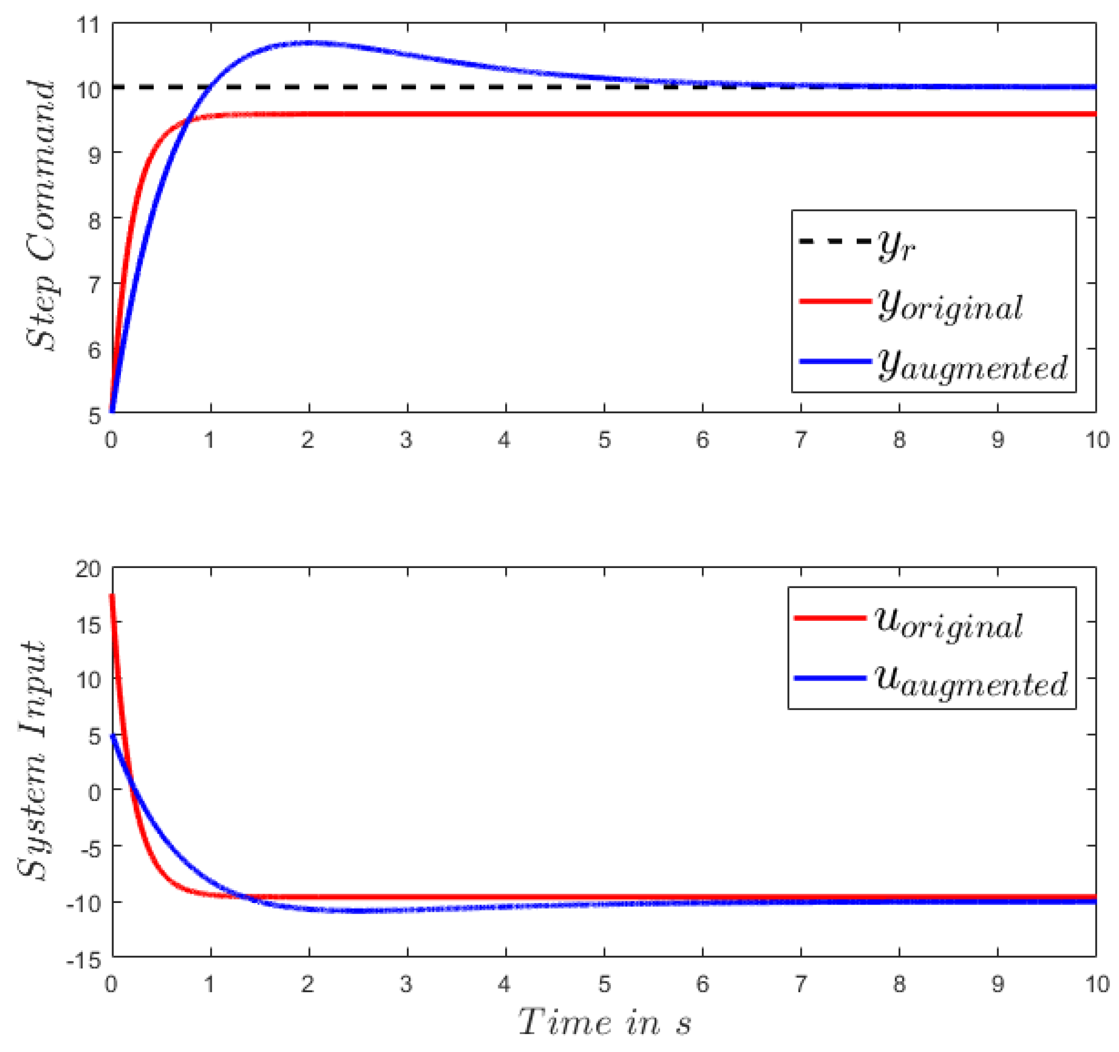
Before we proceed, we implement the method once again in a simple system: a one-dimensional LTI system in the form of (2) with A = 1 , B = 1 , C = 1 . It is unstable in open-loop. This example illustrates the effectiveness of the framework introduced in Section 2.4. Assume that the control target is to track a step command with the final value y r = 10 . Both the LQT control framework with original system and augmented system are implemented. With the same amount of input energy, the differences of the system behavior with the two control laws are compared. As depicted in Figure 2, it is clear to see that zero steady-state error is achieved in the augmented version as expected. However, the transient dynamic is slower and a slight overshoot is observed, compared to the LQT with the original system. For the latter case, an offset to the desired steady-state is apparent. In both cases, the transient dynamic can be changed by tuning the input weighting matrix, but the conclusion made above is not affected.

3. LQT Implementation on Car-in-the-Loop

3.1. Car-in-the-Loop Test Bench Prototype

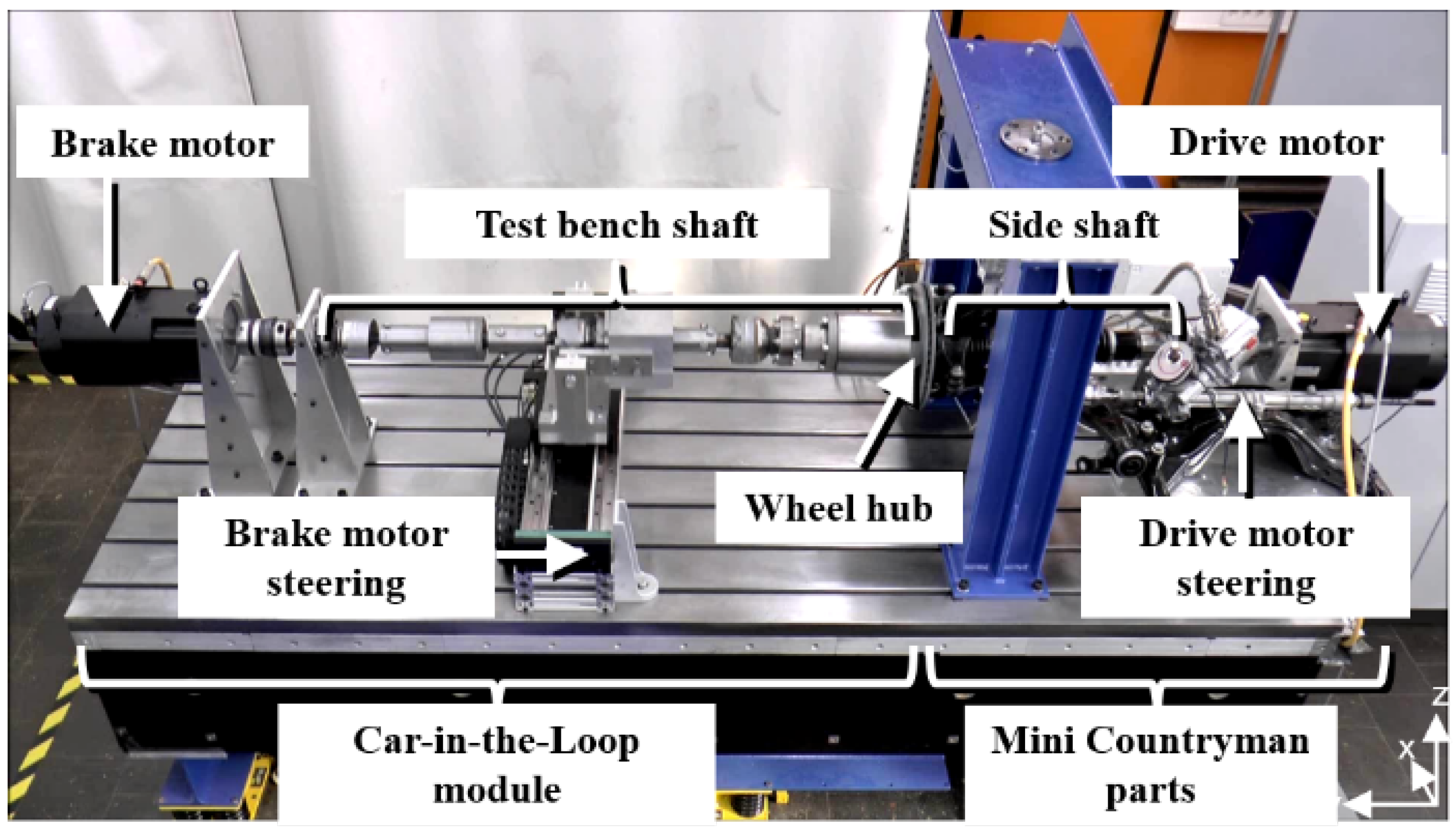
Now we consider a real-world system called Car-in-the-Loop test bench prototype as depicted in Figure 3. For simplification of notation, we refer the system in the following chapters as CiL. More details about the test bench, e.g., the physical parameters, are described in [14]. The control task in this work is to track a reference trajectory of the wheel hub speed using the brake motor torque, while the torque from the drive motor can be seen as a disturbance from the perspective of the test bench control.
In this contribution, to simplify the case study, we neglect the friction and backlash in the system and consider the CiL as an LTI system, which can be described in state-space form as (2) with
A = 0 0 1 1 0 0 0 0 1 1 322277 0 23.24 23.12 0 27038.8 48516.0 1.94 9.24 7.27 0 401767.1 0 60.24 60.32 , B = 0 0 0 0 40.16 T , C = 0 0 0 1 0 T .
The output matrix C hints that only the wheel hub speed among all the five states is measured.
Since the LQT control framework with augmented system has the advantage of zero steady-state error, we adopt this method for the further study on CiL. To be more specific, we augment the system with the integrated tracking error of wheel hub speed as an additional state. Furthermore, we include this state also in the exogenous system and simply assume that it should be constantly zero.
For the case that we have an LQT with a step command of the wheel hub speed, we can construct the exogenous system for the augmented system as the following:
A a ¯ = 0 0 1 0 , C a ¯ = 1 0 0 0 , E d = 0 0 0 0 0 1 0 0 0 0 0 0 T .
And for the augmented system, we construct the weighting matrix of the cost function with Q = diag ( [ Q 1 , Q 2 ] ) and R, with Q 1 being the weighting factor for the tracking error, Q 2 for the augmented state and R for the system input.

3.2. LQT Control with Perfect Model of the Real System

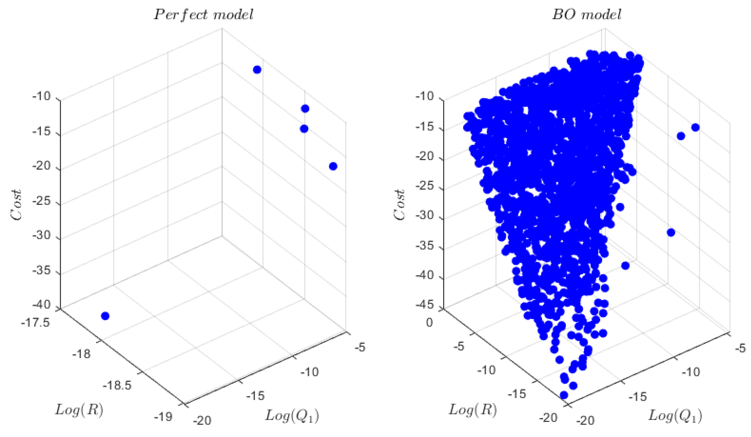
Assume that the real system is completely known, the controllability and observability of the system can easily be examined. Therefore, we can use ( A , B , C ) as the perfect model of the real system to solve the LQT problem as described in Section 2.4, by calculating (12) using (13) and (14), with P and Π ϕ obtained by solving (15) and (16). Due to the characteristic of the system state matrix, it is rescaled for more stable matrix operations. For this specific system, it is proved to be extremely difficult to find a stable control solution using the perfect model of the real system for the control. A Monte-Carlo simulation with a number of 1 e 4 repeats with Q 1 , Q 2 and R randomly selected in the range of 1 e [ 20 , 4 ] is performed. As depicted on the left side of Figure 4, only 5 out of the 1 e 4 random combinations of weighting factors contribute to a stable controller.
From the optimization point of view, the model offers much more degrees of freedom for the problem solving than that of the weighting matrices in the cost function. Abandoning a direct physical interpretation of the model for the controller, in the following chapters we are going to show that a model learnt via Bayesian Optimization (BO) can facilitate a much bigger set of stable controllers. It also exhibits an improved control performance. To the best of the authors’ knowledge, this discovery is the first in the LQT related literature. Before implementing the method on CiL, along with a short discussion on model learning for control, the fundamentals of BO will first be introduced.

4. Model Learning via Bayesian Optimization

Bayesian optimization is a powerful tool, which allows the user to develop a framework to efficiently solve learning problems [15]. Satisfactory results can be obtained within even fewer than 100 iterations [16,17]. Furthermore, it tolerates stochastic noise in function evaluations and is best suited for optimization of system with small to medium sizes, typically less than 20 dimensions [18]. Bayesian optimization is being continuously developed, for an overview to recent advances of the algorithm the readers can refer to [19]. Due to the learning efficiency and noise toleration, it has great potential for industrial implementations, for example in process systems [20,21], positioning system [22] and robotics [23].

4.1. A Short Discussion on Model Learning for Control

With regard to the control of dynamic systems, Bayesian optimization has recently gained increased attention. A great part of it focus on controller parameter tuning [24,25]. In comparison, leveraging BO for model learning is not extensively researched [26,27]. Among the few publications, many of them are focusing on learning a residual model to complement the linear model in the model-based controller scheme, to achieve a better control quality. In [28], the authors use GP to learn the relation between the adaptive term and modelling error in Model Reference Adaptive Control. And in [29], GP is used for real time model adaptation, minimizing the error between prediction and measurement, as a straightforward extension of robust control. Similarly, GP is used to approximate the unknown part of the nonlinear model in [27,30]. According to [31], it is often estimated that 75% of the cost associated to an advanced control project goes into system modeling. From the practical point of view, the proposed methods in literature does not significantly reduce the effort for modeling, since a static nominal model still needs to be identified. On the other hand however, additional effort should be made for the learning procedure. This fact could be a big hazard namely a motivation stopper for the industrial implementation of the proposed advanced controller optimization algorithm.
In general, the majority of the literature in this regard handles the modelling based on the belief of separation principle and certainty equivalence, in case when state estimation is involved. As stated in [32], "a guiding principle should be to model as well as possible before any model or controller simplifications are made as this ensures the best statistical accuracy". So the general consent in the framework of data-driven control is that we also need a perfect model-plant match. There are only very few exceptions in literature that discuss the topic of direct performance-driven model learning under closed-loop conditions [33], where model-plant mismatch could be possible, it is not necessarily examined. In this approach, no or very little prior knowledge with very few implementing cost is required, the model parameters are used directly and purely for the optimization of control performance.
Within the LQT control framework, it turns out that the controller with learnt model can provide significantly more stable solutions for some certain systems, than the controller which has the perfect knowledge of the system. An assumption is that inherently a model-plant mismatch is highly possible for the former case. This fact causes two concerns. The first concern is over-fitting. However, it is shown that with carefully designed experiments, one can learn a data-driven model for control which excites the dynamic spectrum of interest. This is a very useful insight. In fact, the authors encourage readers to use the system itself to (semi-)automatically generate the information of interest [32]. A second concern is the stability margin. In the case of LQG controller, as famously stated in [34], there is none for this class. It means that the stability margin is always system specific. In practical use, we carefully examine the robustness of the controller for individual cases. For CiL, the test scenarios can be categorized in several dynamic range and represented with certain test signals. In this case, the robustness will be examined directly in experimental setup. Examples for systematic study of robustness and integration into the algorithm for data-driven control can refer to [24,30,35]. It is not in the scope of this paper. The intention of the authors is to showcase the possibilities opened up by this new approach, with focus on the industrial practicability.

4.2. Bayesian Optimization with Gaussian Process as Surrogate Model

As hinted in the previous section, in this contribution, we focus on using the BO to learn a system model dedicated for the control task. In other words, it is a performance-driven learning scheme [36]. The learning procedure is summarized in Algorithm 1 and will be explained in detail in the following.
Essentially, BO is an efficient way to learn the relationship between the model parameter θ and the control performance J based on past observations. With random initial model parameters θ 0 , the controller is instantiated and control sequences are applied to the dynamic system. We then evaluate the control performance J 0 ( u 0 , y 0 ) with respect to input energy and tracking error by computing a predefined cost function. Then we obtain our first observation D 0 ( θ 0 ) , with θ 0 hinting the dependencies of the observation on the model parameters. For simplification of notation, in the following, when no misunderstanding occurs, D i ( θ i ) will be simply note as D i . Notice also that without any suffix, the observation D represents the whole set of current observations, same rules apply to other mathematical notations.
We assume that the control performances are random variables that have a joint Gaussian distribution dependent on the model parameters. Without any observation, we define a GP prior that is a Gaussian distribution over function, which is completely parameterized by its mean and variance. Then, we can draw samples from it, which serve as candidate functions for what we are looking for. The actual observation D i is a sample from the distribution of f ( θ i ) . In Bayesian learning, we use the observations to re-weight these function candidates. The probability of a certain candidate function f ( θ ) from the prior is defined as p ( f ( θ ) ) , the Bayes rule
p ( f ( θ ) D ) = p ( D f ( θ ) ) p ( D g ( θ ) ) p ( g ( θ ) ) d g ( θ ) · p ( f ( θ ) )
scales this probability by a factor. The numerator of the scaling factor describes the likelihood of observations given the candidate function. It is normalized by the average likelihood, in other words, the overall probability of our observation over all possible candidate functions.
We are interested in finding the posterior p ( f ( θ * ) D ) because we want to make predictions at the unobserved locations θ * , which in turn will be evaluated by the acquisition function for the decision of where the next iteration is going. We compute the posterior from the prior and the likelihood. By applying the Gaussian marginalization rule we obtain
f ( θ * ) N ( m ( θ * ) , k ( θ * , θ * ) )
Both f ( θ * ) and observations D are Gaussian, by unfolding the definition of covariance and linearity of expectation, their joint distribution can be formulated as follows:
f ( θ * ) D N ( m ( θ * ) m ( θ ) , k ( θ * , θ * ) k ( θ * , θ ) k ( θ * , θ ) T ( k ( θ , θ ) + η 2 I n ) )
By applying the conditional rule for multivariate Gaussian, the distribution for the posterior is obtained:
f ( θ * ) D N ( μ * , σ * 2 )
with the posterior mean μ * :
μ * = m ( θ * ) + k ( θ * , θ ) ( k ( θ , θ ) + η 2 I n ) 1 ( J ( θ ) m ( θ ) )
and posterior covariance σ * 2
σ * 2 = k ( θ * , θ * ) k ( θ * , θ ) ( k ( θ , θ ) + η 2 I n ) 1 k ( θ * , θ ) T
The steps of (23), (25) and (26) are a recurring pattern in Bayesian learning and we use this to compute the posterior for Gaussian process model. By assuming zero mean and expanding (25) we have
μ * = μ 1 * μ 2 * . . . μ n x * = k ( θ 1 * , θ 1 ) k ( θ 1 * , θ 2 ) . . . k ( θ 1 * , θ n T ) k ( θ 2 * , θ 1 ) k ( θ 2 * , θ 2 ) . . . k ( θ 2 * , θ n T ) . . . k ( θ n x * , θ 1 ) k ( θ n x * , θ 2 ) . . . k ( θ n x * , θ n T ) ( k ( θ , θ ) + η 2 I n T ) 1 D 1 D 2 . . . D n T
The expanded mean (27) reveals that for an arbitrary test location θ j * , the posterior is a weighted sum of all the observations D normalized by ( k ( θ , θ ) + η 2 I n T ) . The weights are defined by the kernel between this test location θ j * and all training locations in D. A typical kernel function is the squared exponential kernel with the following structure:
k ( θ j , θ k ) = σ 2 e x p ( ( θ j θ k ) 2 2 l 2 ) ,
with l being the length scale, which characterize how correlated the random variables are depending on the distance, and σ 2 the signal variance, which reflects the range of function values.
Finally, we model the observations as a linear transformation from the latent variable f with added Gaussian noise. The questions arises during this process are how to select the test points for prediction from infinite possibilities in the parameter space and how BO decides the next iteration point, leveraging the information gathered from the GP. To the first question, there are many different search methods introduced in the literature, e.g. "local random search". For the second question, typically, BO decides the next sample location by optimizing the so-called acquisition function α ( θ ) , e.g. Expected Improvement (EI), with the use of the mean and variance predictions of the GP. It selects the next parameter set where the expected improvement over the target minimum among all the explored data is maximal. In this way, the model instance with this new optimal parameter set - up to the current iteration - is used for the controller in the subsequent step.
It is important to note that the decision on the next model parameter set is an internal loop of the BO framework, which does not require experiments on the real system. Therefore, the approach is extremely data efficient. To speed up the algorithm’s convergence, one can also set constraints on the search space of the model parameters based on prior knowledge to the system. For example, the signs of certain parameters can be predetermined, when their meaning can be physically interpreted.

5. LQT Implmentation on Car-in-the-Loop Revisited

Recall that in Chapter Section 3, we can scarcely find stable controllers by implementing LQT with augmented states on CiL with perfect knowledge of the ’real’ system. In other words, we use a perfect model of the ’real’ system for the controller in the simulation study. Now we revisit the CiL control problem and implement the algorithm of model learning via BO as described in Algorithm 1 on the simulated test bench.
Algorithm 1: Model learning via Bayesian Optimization
Step Procedure
1 Initialize GP with D 0 = J 0 ( θ 0 )
2 for i = 1 : N 1
find θ * = a r g m a x α ( θ | D ) , a p p l y θ i θ *
conduct closed-loop experiment with S ˜ ( θ i )
measure u i and y i ;
compute cost function J i
update GP and D with θ i , J i
3 Compute optimal parameter θ i * , where i * = a r g m i n J i .

5.1. LQT with Model Learnt via BO

To be more specific, we use the BO to learn the system state matrix A B O and input matrix B B O for the LQT controller directly in closed-loop conditions. With trivial weighting of Q 1 = 1 , Q 2 = 8 and R = 1 and random initialization, we obtain the following BO model ( A B O , B B O ) for the LQT control:
A B O = 0 0 1 1 0 0 0 0 1 1 565390 0 490.92 106.63 0 824120 563610 323.5 475.87 278.53 0 271700 0 314.96 83.672 , B B O = 0 0 0 0 95.36 T .
This model will be called BO model in the following sections for simplification of notation.
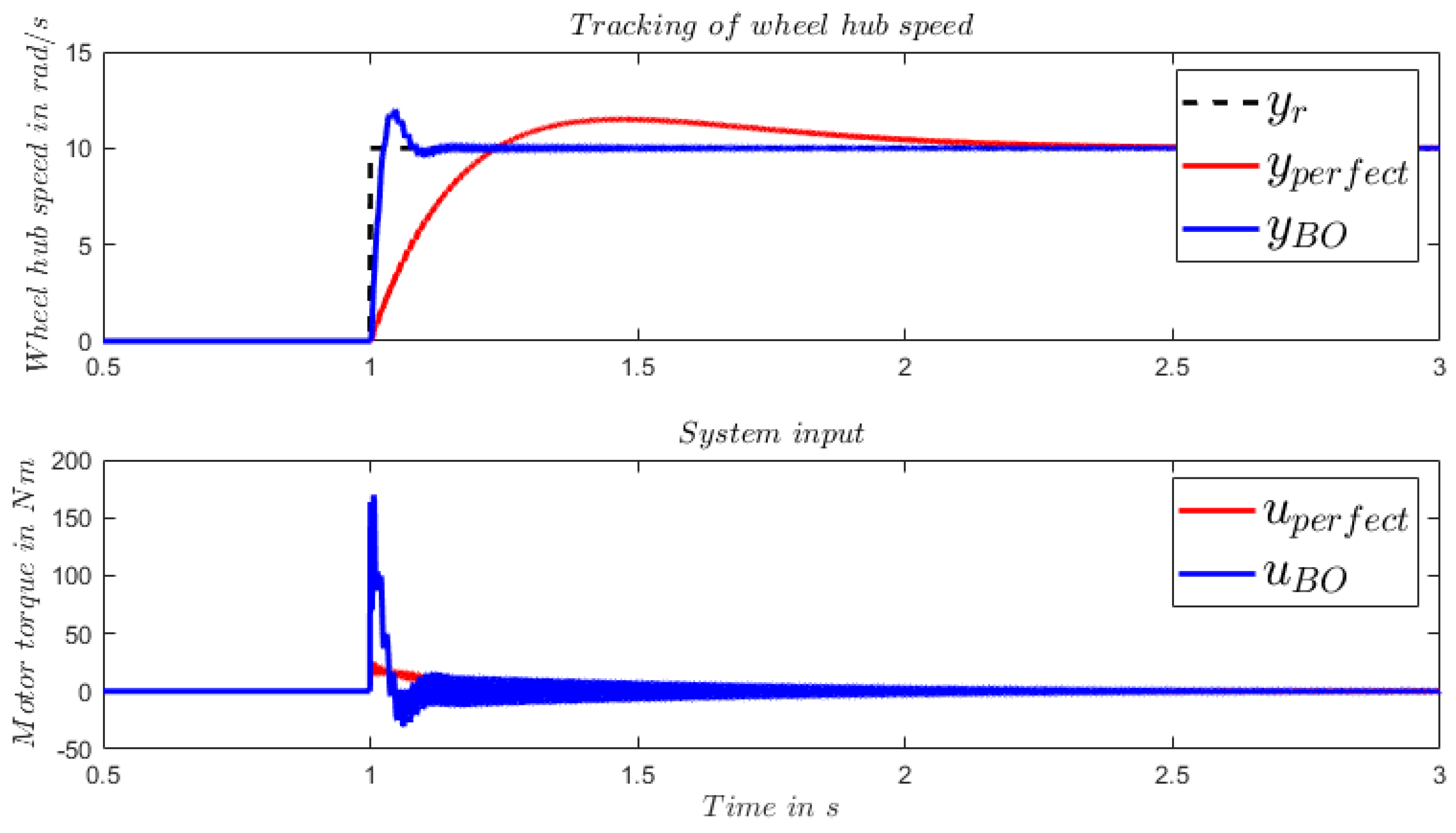
A Monte-Carlo simulation with the same settings as described in Chapter Section 3 is performed and the simulation results are illustrated on the right side of Figure 4. In total, 1782 stable controllers are obtained, which is a significant improvement compared to the sparse stable controller set with the perfect model of the ’real’ system. In Figure 5, a comparison of the step command response is depicted. The best result with the perfect model (lower left point in the left plot of Figure 4) is shown in red color. A representative point with comparable overall cost from the results with BO model is presented in blue. As illustrated, the controller with BO model injects more energy to the system to allow a much faster transient dynamic.
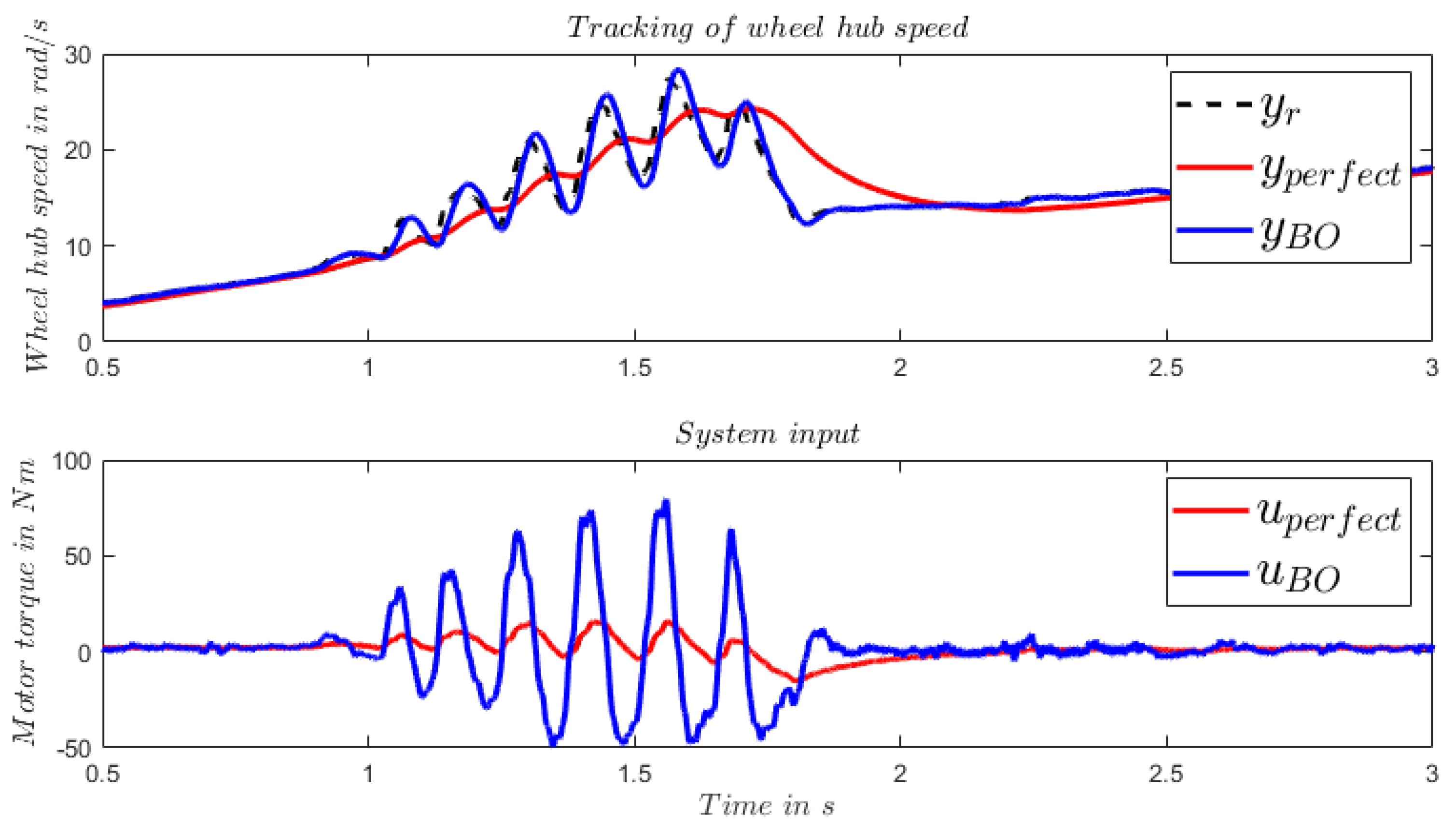
In practice, it is difficult to describe an arbitrary reference trajectory of wheel hub speed, i.e., the vehicle velocity with the formulation of (10). It is trivial to consider the reference trajectory as small step commands in each sample time and therefore, one can use the same controller for an arbitrary reference trajectory as for the step command. The practicability of this simplification is validated using a recorded wheel hub speed from real world driving as reference trajectory, where the tire slip phenomenon is captured. The results are illustrated in Figure 6. Due to the much faster transient dynamic, the controller with BO model tracks the reference trajectory much better than its counterpart with the perfect model.

5.2. Effectiveness of Bayesian Learning

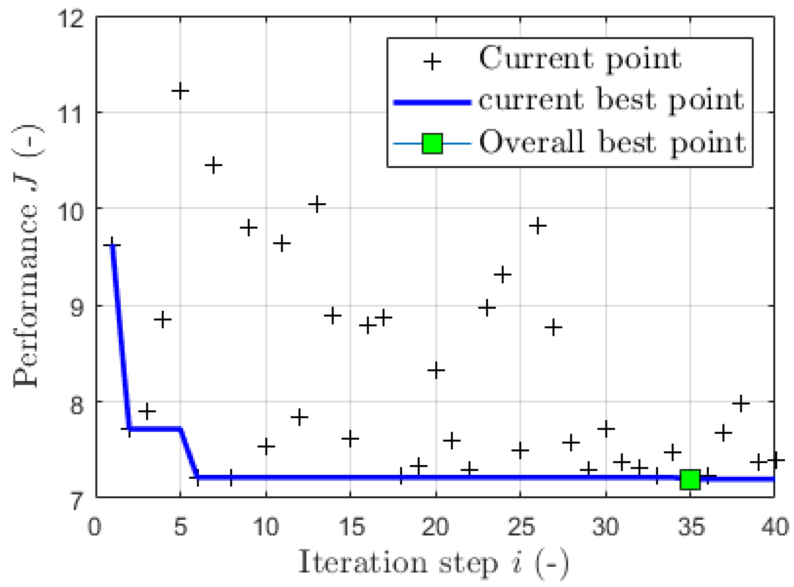
The BO algorithm for model learning converges fast in the case of CiL. In Figure 7, a representative closed-loop system performance of CiL in simulation over the iteration steps during the model learning is illustrated. The blue line visualizes the current best performance up to iteration i. With enough initial seeds of parameter sets randomly selected from the parameter space, the BO algorithm converges in a very effective manner. Therefore, in the case of CiL, the performance-driven approach together with BO is data-efficient and suitable for experimental controller design.

5.3. Limitations

Currently the introduced method is studied in the simulation environment, where all the system states are assumed known. Nonlinear effects of the real system are not considered. Since not all the system states can be measured, the feasibility of the method and stability of the controller with a state estimator needs further investigation, to pace the way for its implementation on the real system. Moreover, due to the state augmentation as well as the introduction of the exogenous system, the dimensions involved in the controller design can increase significantly for systems with high dimension and/or multiple tracking states.

6. Conclusion

In this contribution, we discuss a control method for LQT with zero steady-state error. It is realized by augmenting the system state with the integrated tracking error. The general LQT control framework introduced in [7] can be used for the augmented system, which is not mentioned in the literature.
A possible reason could be that due to the augmentation of the system as well as the introduction of the exogenous system, the dimension of the Sylvester equation (16) could be increased quite significantly, when many states or outputs are to be tracked in the system. This fact could be a limitation of the method.
On the other hand, an interesting discovery is, for the specific system CiL, that nearly no stable solution can be found with the perfect model of the ’real’ system for the LQT control. However, a stable and more performing solution can be found more easily with a plant model learnt via BO. Based on the learnt model, the controller parameter can be further tuned in a sequential step and achieve a desired performance with regard to certain objective.
Currently, the conclusions made in this contribution are based on numerical simulations. All system states are assumed known. In future works, the control method in combination with a state estimator should be studied further to pave the way for its practical use. It is also interesting to prove the feasibility or stability of the method mathematically in a more general term. For example, how can the BO model as a substitute model provide an alternative way to the LQT controller design for a certain class of system similar to CiL, which is scarcely unsolvable with the perfect model of the ’real’ system.

References

  1. Schyr, C.; Inoue, H.; Nakaoka, Y. Vehicle-in-the-Loop Testing - a Comparative Study for Efficient Validation of ADAS/AD Functions. 2022 International Conference on Connected Vehicle and Expo (ICCVE). IEEE, 07.03.2022 - 09.03.2022, pp. 1–8. [CrossRef]
  2. Peter Bauer. Development and performance evaluation of an infinite horizon LQ optimal tracker.
  3. Park, J.H.; Han, S.; Kwon, W.H. LQ tracking controls with fixed terminal states and their application to receding horizon controls. Systems & Control Letters 2008, 57, 772–777. [Google Scholar] [CrossRef]
  4. Willems, J.L.; Mareels, I.M. A rigorous solution of the infinite time interval LQ problem with constant state tracking. Systems & Control Letters 2004, 52, 289–296. [Google Scholar] [CrossRef]
  5. Modares, H.; Lewis, F.L. Linear Quadratic Tracking Control of Partially-Unknown Continuous-Time Systems Using Reinforcement Learning. IEEE Transactions on Automatic Control 2014, 59, 3051–3056. [Google Scholar] [CrossRef]
  6. HAGIWARA, T.; YAMASAKI, T.; Araki, M. Two-degree-of-freedom design method of LQI servo systems: disturbance rejection by constant state feedback. International Journal of Control 1996, 63, 703–719. [Google Scholar] [CrossRef]
  7. Bernhard, S. Time-Invariant Control in LQ Optimal Tracking: An Alternative to Output Regulation. IFAC-PapersOnLine 2017, 50, 4912–4919. [Google Scholar] [CrossRef]
  8. Enrique Barbieri. On the infinite-horizon LQ tracker 2000.
  9. YOUNG, P.C.; WILLEMS, J.C. An approach to the linear multivariable servomechanism problem†. International Journal of Control 1972, 15, 961–979. [Google Scholar] [CrossRef]
  10. Fietzek, R.; Rinderknecht, S. Hardware-in-the-Loop test rig for driver assistance systems and autonomous vehicles 2015.
  11. Malkapure, H.G.; Chidambaram, M. Comparison of Two Methods of Incorporating an Integral Action in Linear Quadratic Regulator. IFAC Proceedings Volumes 2014, 47, 55–61. [Google Scholar] [CrossRef]
  12. Singh, A.K.; Pal, B.C. An extended linear quadratic regulator for LTI systems with exogenous inputs. Automatica 2017, 76, 10–16. [Google Scholar] [CrossRef]
  13. Mukherjee, S.; Bai, H.; Chakrabortty, A. Model-based and model-free designs for an extended continuous-time LQR with exogenous inputs. Systems & Control Letters 2021, 154, 104983. [Google Scholar] [CrossRef]
  14. S. Rinderknecht, R.F. Control Strategy for the Longitudinal Degree of Freedom of a Complete Vehicle Test Rig 2012.
  15. Brochu, E.; Cora, V.M.; Freitas, N.d. A Tutorial on Bayesian Optimization of Expensive Cost Functions, with Application to Active User Modeling and Hierarchical Reinforcement Learning.
  16. Khosravi, M.; Koenig, C.; Maier, M.; Smith, R.S.; Lygeros, J.; Rupenyan, A. Safety-Aware Cascade Controller Tuning Using Constrained Bayesian Optimization. IEEE Transactions on Industrial Electronics. [CrossRef]
  17. Fröhlich, L.P.; Küttel, C.; Arcari, E.; Hewing, L.; Zeilinger, M.N.; Carron, A. Model Learning and Contextual Controller Tuning for Autonomous Racing.
  18. Frazier, P.I. A Tutorial on Bayesian Optimization.
  19. Wang, X.; Jin, Y.; Schmitt, S.; Olhofer, M. Recent Advances in Bayesian Optimization. ACM Computing Surveys 2023, 55, 1–36. [Google Scholar] [CrossRef]
  20. Paulson, J.A.; Tsay, C. Bayesian optimization as a flexible and efficient design framework for sustainable process systems.
  21. Coutinho, J.P.; Santos, L.O.; Reis, M.S. Bayesian Optimization for automatic tuning of digital multi-loop PID controllers. Computers & Chemical Engineering 2023, 173, 108211. [Google Scholar] [CrossRef]
  22. Koenig, C.; Ozols, M.; Makarova, A.; Balta, E.C.; Krause, A.; Rupenyan, A. Safe Risk-averse Bayesian Optimization for Controller Tuning.
  23. Wabersich, K.P.; Taylor, A.J.; Choi, J.J.; Sreenath, K.; Tomlin, C.J.; Ames, A.D.; Zeilinger, M.N. Data-Driven Safety Filters: Hamilton-Jacobi Reachability, Control Barrier Functions, and Predictive Methods for Uncertain Systems. IEEE Control Systems 2023, 43, 137–177. [Google Scholar] [CrossRef]
  24. Stenger, D.; Ay, M.; Abel, D. Robust Parametrization of a Model Predictive Controller for a CNC Machining Center Using Bayesian Optimization. IFAC-PapersOnLine 2020, 53, 10388–10394. [Google Scholar] [CrossRef]
  25. Neumann-Brosig, M.; Marco, A.; Schwarzmann, D.; Trimpe, S. Data-Efficient Autotuning With Bayesian Optimization: An Industrial Control Study. IEEE Transactions on Control Systems Technology 2020, 28, 730–740. [Google Scholar] [CrossRef]
  26. Sorourifar, F.; Makrygirgos, G.; Mesbah, A.; Paulson, J.A. A Data-Driven Automatic Tuning Method for MPC under Uncertainty using Constrained Bayesian Optimization. IFAC-PapersOnLine 2021, 54, 243–250. [Google Scholar] [CrossRef]
  27. Chakrabarty, A.; Benosman, M. Safe Learning-based Observers for Unknown Nonlinear Systems using Bayesian Optimization.
  28. Robert, C. Grande, Girish Chowdhary, Jonathan P. How. 2014_Experimental_Validation_of_Bayesian_ Nonparametric Adaptive Control Using Gaussian Processes_ctn25.
  29. Bart, M. Doekemeijer.; Daan C. van der, Hoek., Jan-Willem van Wingerden. Model-based closed-loop wind farm control for power maximization using Bayesian Optimization using BO: 3rd IEEE Conference on Control Technology and Applications : August 19-21, 2019, City University of Hong Kong, Eds.; IEEE: Piscataway, NJ, 2019. [Google Scholar] [CrossRef]
  30. Berkenkamp, F.; Schoellig, A.P. Safe and robust learning control with Gaussian processes. 2015 European Control Conference (ECC). IEEE, 15.07.2015 - 17.07.2015, pp. 2496–2501. [CrossRef]
  31. M. Gevers. Identification_for_Control_From_the_Early achievements to the revival of experiments design_ctn354 2005.
  32. Hjalmarsson, H. From experiment design to closed-loop control. Automatica 2005, 41, 393–438. [Google Scholar] [CrossRef]
  33. Bansal, S.; Calandra, R.; Xiao, T.; Levine, S.; Tomlin, C.J. Goal-Driven Dynamics Learning via Bayesian Optimization.
  34. Doyle, J. Guaranteed margins for LQG regulators. IEEE Transactions on Automatic Control 1978, 23, 756–757. [Google Scholar] [CrossRef]
  35. Alanwar, A.; Stürz, Y.; Johansson, K.H. Robust Data-Driven Predictive Control using Reachability Analysis.
  36. Piga, D.; Forgione, M.; Formentin, S.; Bemporad, A. Performance-Oriented Model Learning for Data-Driven MPC Design. IEEE Control Systems Letters 2019, 3, 577–582. [Google Scholar] [CrossRef]
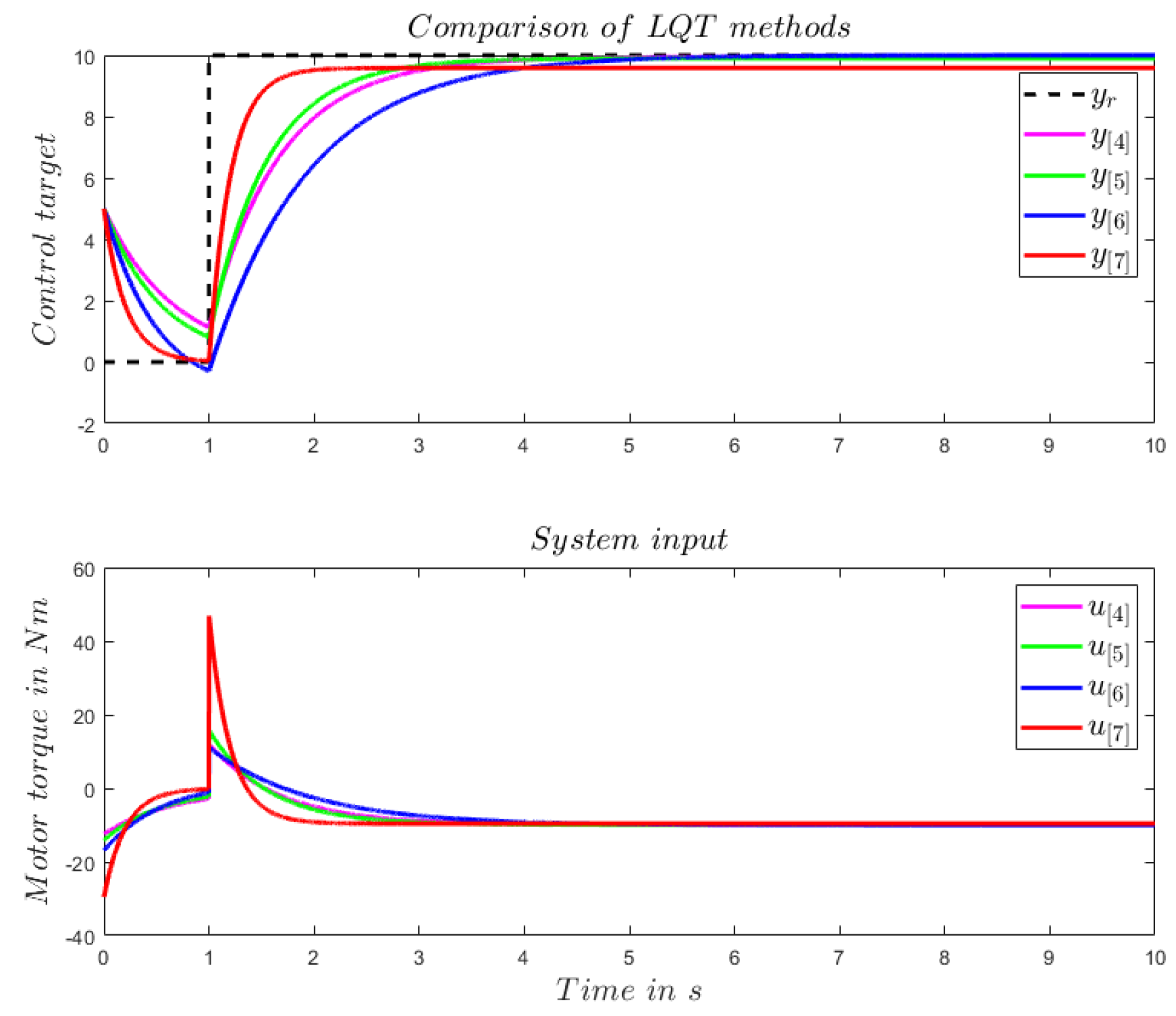
Figure 1. Tracking of a step command by an LTI system with A = 1, B = 1 and C = 1 using different LQT control methods mentioned above. The same amount of input energy is injected to the system for all control methods: [4,5,6,7].
Preprints 110179 g001
Figure 2. Tracking of a step command by an LTI system with A = 1 , B = 1 , C = 1 . LQT control framework with original system model (red line) and augmented system model (blue line) are implemented. Same amount of input energy is injected to the system in both control laws.
Preprints 110179 g002
Figure 3. Car-in-the-Loop test bench prototype.
Preprints 110179 g003
Figure 4. Stable controller set with Monte Carlo Simulation. Q 1 , Q 2 and R are randomly selected in the range of 1 e [ 20 , 4 ] . For ease of reading, the cost evaluation is averaged over the sample numbers and logarithmized. Left: stable controller set with perfect model of the real system, right: stable controller set with learnt model via BO.
Preprints 110179 g004
Figure 5. Comparison of the step command response with LQT control framework using perfect model of the ’real’ system and the BO model. Overall cost for both controllers is comparable.
Preprints 110179 g005
Figure 6. Comparison of the tracking of real measurement data with LQT control framework using perfect model of the ’real’ system and the BO model.
Preprints 110179 g006
Figure 7. Iteration of the Bayesian optimization algorithm.
Preprints 110179 g007
Disclaimer/Publisher’s Note: The statements, opinions and data contained in all publications are solely those of the individual author(s) and contributor(s) and not of MDPI and/or the editor(s). MDPI and/or the editor(s) disclaim responsibility for any injury to people or property resulting from any ideas, methods, instructions or products referred to in the content.
Copyright: This open access article is published under a Creative Commons CC BY 4.0 license, which permit the free download, distribution, and reuse, provided that the author and preprint are cited in any reuse.
Prerpints.org logo

Preprints.org is a free preprint server supported by MDPI in Basel, Switzerland.

Subscribe

© 2024 MDPI (Basel, Switzerland) unless otherwise stated