Preprint
Article

Research on Optimizing Human Resource Expenditure in the Allocation of Materials in Universities

Altmetrics

Downloads

68

Views

20

Comments

0

A peer-reviewed article of this preprint also exists.

This version is not peer-reviewed

Submitted:

27 June 2024

Posted:

27 June 2024

You are already at the latest version

Alerts
Abstract
This study establishes a multivariate function model for natural human load carrying walking in some typical scenarios like college equipments and materials relocation for students. For classified materials relocation needs and constraints, we obtain the relationship between walking speed and load weight for single person, as well as the time cost for different round trips. By establishing an integer programming model with the minimum total transportation time cost and quality assurance as the objective function and the requirements of negative weight and speed as the constraints conditions, we reach the optimal item allocation methods considering time cost and shelf life were obtained. We discover that there is an approximate linear relationship between the change in natural walking speed and travel time when the load is small, thus obtaining the time cost of student transportation under different round-trip situations. The Monte Carlo simulation algorithm is used to obtain the optimal allocation scheme that meets the efficiency and quality requirements. The analysis methods and results can be used as guidance for task scheduling optimization for material relocation in educational organizations as well as commercial agencies.
Keywords: 
Subject: Computer Science and Mathematics  -   Information Systems

1. Introduction

1.1. Background of the Problem

In the context of constantly escalating logistic demand, the logistics problem is gradually emerging and developing rapidly. For example, logistic problems are typical in colleges. For example in China colleges with the increase of online shopping, increasing quantities of parcels pour into campus daily, one or more large scale parcels distribution center established in single campus, compared with that many city blocks share only one small distribution center in city area. Also with fast Universities development in China, constant facilities upgrade or new campus plan call for many freight relocation needs, for example, the new University level physics experiment classrooms relocation call large scale teaching equipments relocation. The University hosted national academic conference call large scale logistic materials transportation. Almost in all such scenarios for freight transportation, at least partial of the relocation trip require manual labor for transport[1,2,3], like when complicated geographical location or unmovable obstacles involved. So there are general needs regarding the specified freight information and sorted relocation need information, to develop efficient relocation scheme to optimize the relocation task[4,5], partially to meet some stringent timing restriction and minimum human and financial resources expenditure.
The general problem is that, depending the information of different items to be relocated and details of resources dispatch requirement, University logistic unit, for example, try to develop corresponding solutions. For items such as vegetables or fresh-keeping items, special attention should be paid to the issue of squeezing and maintaining quality and efficiency during transportation. In some special road sections or situations, manual load consumption may be high, and students (in Universities where transportation tools have objective restriction) need to be transported one or more times with heavy loads[6,7,8]. Logistics units need to further optimize personnel configuration and focus on sorting and distribution. How to build a logistics distribution and allocation model that meets the requirements, improve the level of logistics services, and propose solutions for the logistics distribution model[9,10,11,12,13] to achieve the highest resource utilization rate is of great significance for the development of the logistics problem today not only in Universities but also in commercial location with special needs.

1.2. Problem Formulation

We adapt to one typical problem scenario, the methodology introduced can be easily extended to different combination of problem parametric values setting[14,15,16]. The following problem, which is representative of a vast category of similar problems, is stated as (considering the sample data in Appendix):
Scheduling task one:Establish a dual leg weight-bearing walking model, study the relationship between the natural walking speed and the weight carried by 9 students carrying different mass items in a short period of time, and predict the changes in the speed of the second and third equal weight-bearing round trips, namely the change in time cost. Scheduling task two:Based on the results obtained from task one, distribute all 16 freight packages to 9 or fewer transport workers once or multiple times.Establish a mathematical model to determine the method of assembling and matching transportation packages for the student with the lowest transportation cost (each time). Scheduling task three: Distribute all 16 freight packages to 9 or fewer transport workers once or multiple times.Establish a mathematical model to determine the mixed solution with the highest number of transportation packages with an average shelf life rate (yield) exceeding 80%, and provide the shelf life rate for each transportation package.

2. Models and Methods

2.1. Problem Analysis

2.1.1. Analysis of Task One

Regarding the analysis of problem one, natural walking is a special way of walking. Through literature review, it is known that at any given speed, the oxygen consumption required for a freely chosen step rate is the smallest, and there is a direct correspondence between the load and the walking rate[17,18,19]. A multivariate process group can be established. According to question one, it can be seen that each student knows 2 sets of natural walking data. Based on the known data, the unknown variables of the relevant equation system are eliminated, and then the data of students with the same characteristics are connected for solving. Finally, the relationship between the natural walking speed and the weight carried[20,21,22,23] by each group of students in a short period of time is obtained. At the same time, through literature review, it is known that there is a correlation between the speed of natural walking and the travel time during long-term travel, which can be used to obtain the changes in the speed of the second and third round trips with equal load.

2.1.2. Analysis of Task Two

For the analysis of question one, it is required to allocate all 16 freight packages to 9 or fewer transport workers based on the results obtained from question one.It is known that the cost of human transportation is directly related to the cost of transportation time. In the process of solving problem one, the relationship between student transportation time cost and load and transportation time is known. Based on this, the objective function of a single objective programming model can be established, which is to minimize the total transportation time. Meanwhile, as the impact of item type on transportation time is not considered, the optimal allocation method for items can be directly calculated multiple times using Monte Carlo simulation algorithm with the student’s load-bearing capacity as the constraint condition.

2.1.3. Analysis of Task Three

Regarding the analysis of question three, as the weight and shelf life of each item are fixed, different types of items are assigned to 9 or fewer transporters. During the mixed allocation process, the shelf life of the transport package changes, so the items can be combined and allocated based on weight. Due to the neglect of transportation time cost and item quality, a single objective programming model can be established, with the objective function of maximizing the number of transportation packages with a quality assurance rate exceeding 80%, and using the student’s load-bearing capacity as a constraint. The Monte Carlo simulation algorithm can be used for multiple simulation calculations to obtain the optimal allocation method and the quality assurance rate of each transportation package.

2.2. Model Assumptions and Symbols Description
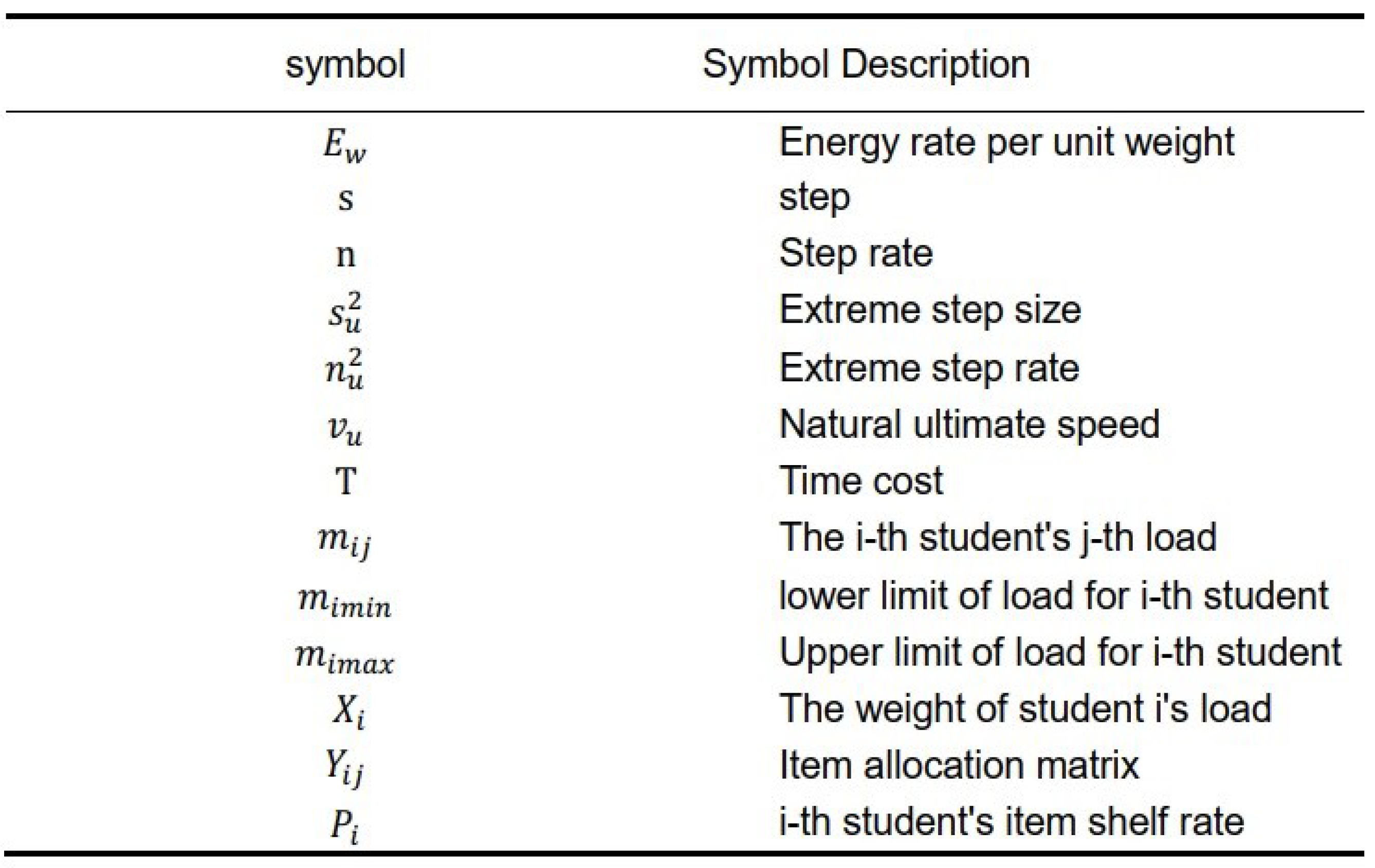
1. Assuming that the physical factors of students are only related to the data table and meet the requirements of the experimental model;
2. Assuming that there is no strict adherence to natural speed during student transportation;
3. Neglecting objective factors beyond the set conditions during transportation;
4. Assuming that the weight of an item can be infinitely divided.
Table 1. Symbols Description.
Preprints 110488 i001

2.3. Establishment and Solution of the Model for Task One

2.3.1. Analysis and Solution of Task One

For question one, it can be seen that 9 students used natural walking mode during the transportation process. By consulting relevant literature and experimental reports on this mode, the relationship between natural walking time and load weight can be obtained, and relevant model equations can be established based on this. At the same time, due to the correlation between students’ empty transportation time, the model equation can be further simplified and solved based on this.

2.3.2. Model Preparation-Energy Consumption Model for Natural Walking

The energy consumption during walking is usually expressed as a function of walking speed. However, this relationship only applies to the stride frequency pattern during natural walking, used to predict the energy consumption of any combination of stride length and stride frequency. Literature review indicates that the energy demand for this combination can be determined through two experiments. In the first scenario, the subjects are free to choose their own walking mode to achieve the specified speed. In the second scenario, the speed remains constant, but the subject is forced to use the prescribed range of step rates. The combination of the results of these two experiments has generated enough data to make it possible to determine the energy equation for patterns, including "free" and "forced" gaits. The results indicate that at any given speed, the oxygen consumption required for a freely chosen step rate is the smallest. Any other forced step rate at the same speed will increase the cost of oxygen, exceeding the oxygen cost required for natural step rates. Research has shown (Zarrugh et al., 1974) that in natural conditions, the total energy consumption during horizontal walking at all stride and speed is
E w = E 0 / ( 1 s 2 / s u 2 ) ( 1 n 2 / n u 2 )
where E w is energy rate per unit weight, in cal/kg/min, s is the step length in meters, N is the step rate in steps per minute, s u is the limit step size in meters, n u is the step rate measured in steps per minute, v u is moving speed, the energy consumption rate at t = 0 is E 0 . The condition for the minimum E derived from equation (1) is applicable to a fixed velocity v, which has been proven to be
s = ( s u / n u ) n
Research has shown that the minimum E w occurs at v = v u / 3 , where v = s n u . If the speed remains constant, the minimum E w step size for that speed needs to be proportional to the step length, and the proportional constant s u / n u remains the same regardless of the speed.
When the subject walks freely, they usually adopt a pattern that is almost identical to the one described in Equation (2).Figure 1 shows the s/n walking mode of the example.A bold continuous line was drawn in the form of Equation (2).The sin relationship shown in Figure 1 is basically linear for all subjects, but there are significant differences between subjects (such as B, C, and G). However, due to a 10% increase in the s/n ratio of typical subjects (walking speed = V u = 80 m / m i n ), energy expenditure only increased by 0.7% compared to the optimal level. Therefore, subjects can change their walking mode near the optimal ratio without significantly increasing their energy expenditure. At the same speed, even if sin increases by 20%, it will only increase by 2.6%. In natural walking, step length is uniquely correlated with step frequency through Equation (2). If speed is chosen as the independent variable and Equation (2) is used, Equation (1) will be simplified to the following natural walking equation:
E w = E 0 / ( 1 v / v u )
where v is walking speed in unit m/min.

2.4. Establishment of Energy Consumption Model for Load Travel of Task One

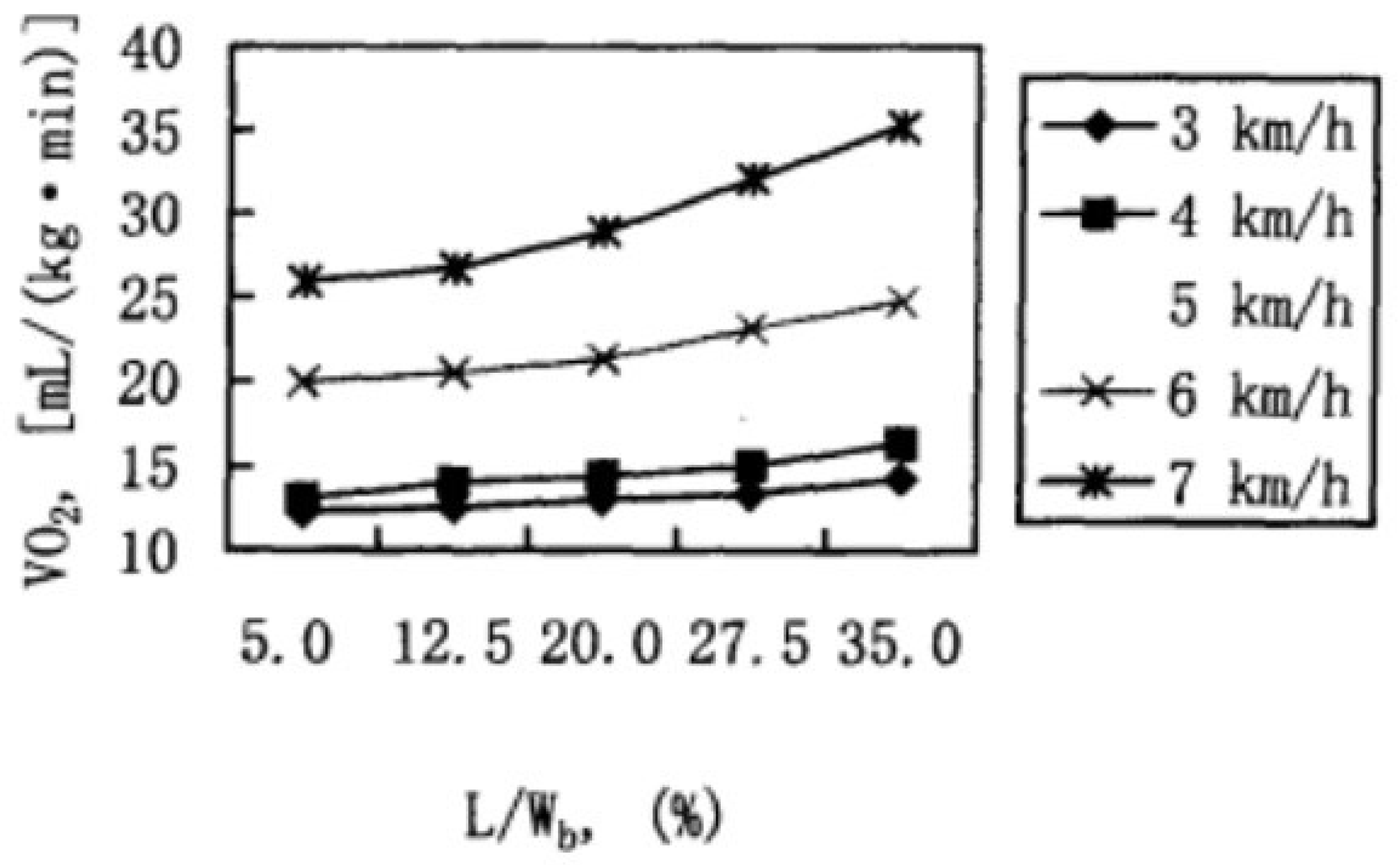
The relationship between oxygen consumption V O 2 [mL/kg. min] and load L / W b (%) at various speed levels is shown in Figure 2, using the mean measured values of 12 subjects as the experimental results.
The results in Figure 2 indicate that the relationship between oxygen consumption (VO) and load (LW) during flat ground load travel should be strictly nonlinear. But when the speed is low, for example: V < 5 k m / h , the relationship is basically linear, and when the speed is high, the nonlinear relationship will gradually become significant. There have been many studies on weight-bearing travel and some empirical equations have been proposed to represent this relationship, with international legal units being used uniformly. Some of the main equations are as follows:
M / W b = ( 1 + L W b ) [ 2 . 7 + 3 . 2 ( V 0 . 7 ) 1 . 65 + G ( 0 . 23 + 0 . 29 ( V 0 . 7 ) ) ] 1 . 3
When G = 0 , there is
M / W b = 1.5 + 2 ( 1 + L W b ) ( L / W b ) 2 + 1.5 V 2 ( 1 + L / W b )
The empirical equation indicates that there is a basic linear relationship between V O 2 and L / W b .However, from the research results, it can be seen that for flat terrain, when V is very high or L / W b very large, the nonlinear relationship between V O 2 and L / W b will gradually become significant (Figure 1). Some studies have also found that the energy consumption during flat ground moving is not always linearly related to the load. It has pointed out that when the load is greater than 40% to 45% of the body weight, the energy consumption during driving will increase nonlinearly, and when the load is larger, the energy consumption will increase faster.
Considering that all 9 students are moving objects at a natural walking speed, the equation system can be obtained by combining equations (3) and (5) as,
{ (6a) 2 E w = E 0 / ( 1 v / v u ) (6b) E w / W b = 1.5 + 2 ( 1 + L W b ) ( L / W b ) 2 + 1.5 V 2 ( 1 + L W b )
Meanwhile, due to the same natural time cost for the first empty load of every three passengers, it can be inferred that the maximum speed v u is the same.The function relationship between the natural walking speed and the load of the i-th student carrying items of different masses in a short period of time, without considering the influence of load time on the natural walking speed, can be obtained as follows
E 0 i / ( 1 v / v u j ) / W b i = 1.5 + 2 ( 1 + L W b i ) ( L / W b i ) 2 + 1.5 V 2 ( 1 + L W b i )
where v is the speed of item handling, L is the mass of item. If we consider the cost of transportation time under the influence of time, as the quality of the goods is much lower than 40% of the weight of the transporter themselves, the transportation time can be regarded as positively correlated with the rate of physical exertion, which can be calculated linearly by 2.6%.

2.5. Solving the Model for Task One

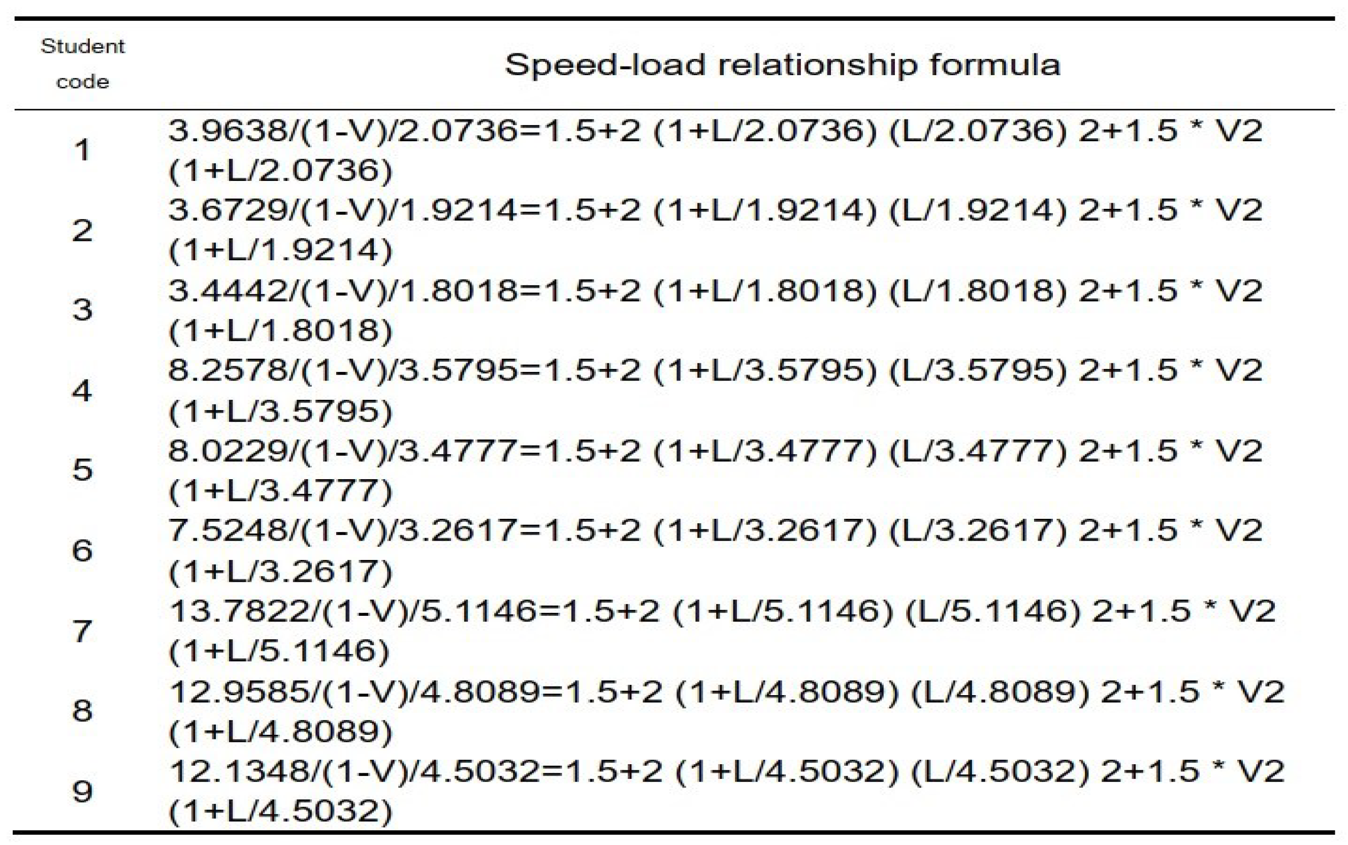
Due to the fixed transportation distance, if the distance is considered as a unit length, then v = 1 / one-way time cost. Using programming software to numerically solve the model, the relationship between the natural walking speed of students and their weight is obtained as shown in the table below.
Table 2. Student Speed-Load Relationship.
Preprints 110488 i002
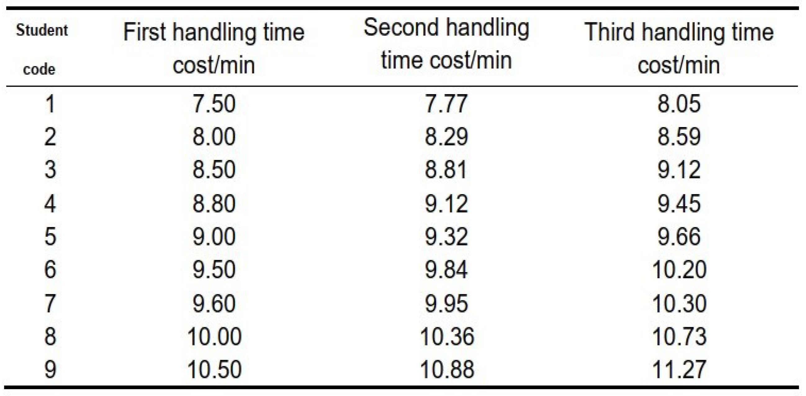
Considering that the physical exertion during unloaded natural walking can be ignored, the time cost under load is linearly correlated with the speed of physical exertion. After calculation, the time cost for each load stage is shown in the table below.
Table 3. Time cost for each round trip stage.
Preprints 110488 i003

2.6. Conclusion of Model for Task One

According to the above analysis, it can be seen that under natural walking conditions, there is a corresponding relationship between time cost and speed. In the case of small loads, the increase in transportation time cost is linearly correlated with transportation time.

2.7. Analysis for Task Two

For question two, it can be seen that the transportation process still adopts a natural walking mode. From question one, the relationship between transportation speed and load weight in this mode is known. Considering that the impact of item types on transportation time and cost can be ignored, the establishment of a single objective programming model mainly considers the relationship between transportation time, load weight, and transportation frequency for 9 students.

2.8. Model Establishment for Task Two-Data Preprocessing
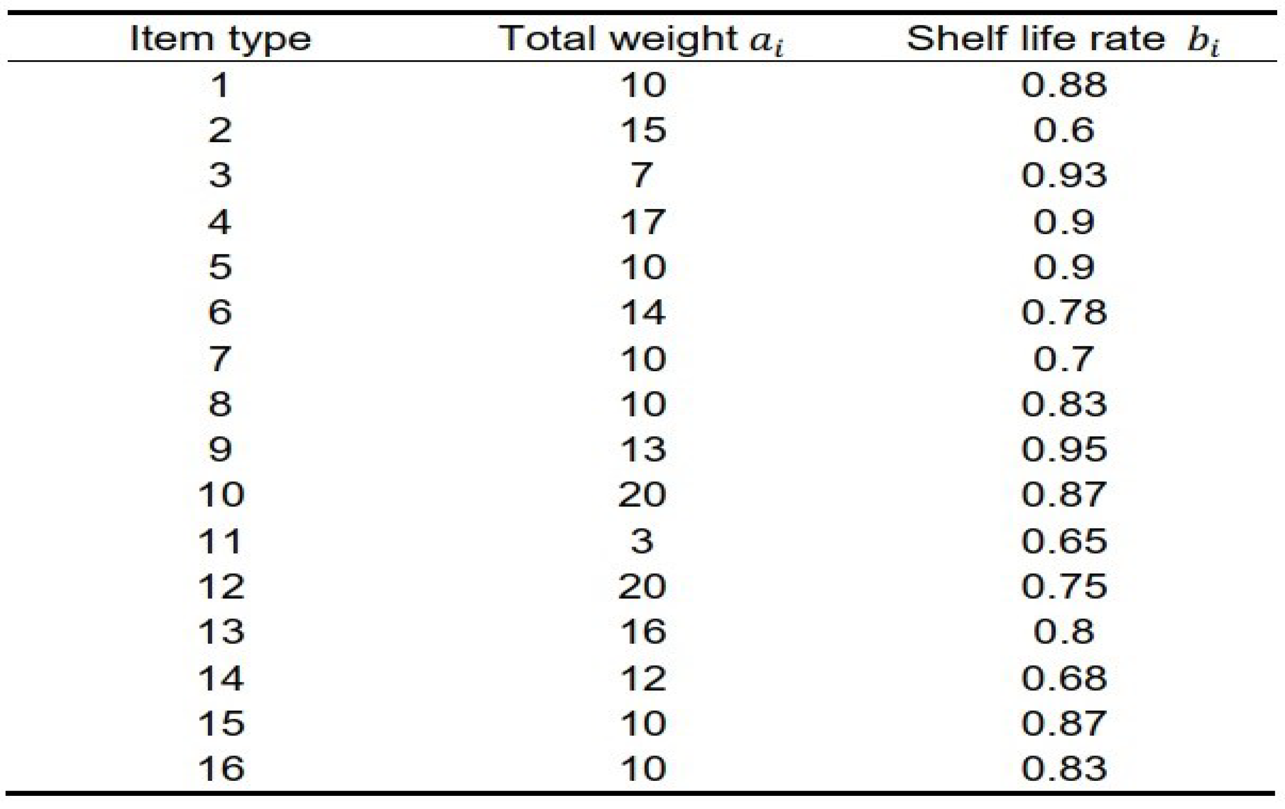
The total mass of the i-th item is a i , and its shelf life rate is b i , both of which are constant real numbers. The values are shown in the table below.
Table 4. Total Weight and Shelf Life of Items.
Preprints 110488 i004
Due to the lack of consideration for transportation time costs and the fact that the student load limit is greater than the total mass of the item, it is assumed that students will only participate in a single transportation activity. If the transportation weight of the i-th student is X i , then
X i = Σ i = 1 16 Y i j a j
where Y i j is coefficient matrix to be determined.

2.9. Model for Task Two

Due to limitations in the number and handling capacity of students, with their load-bearing capacity as the limiting condition and the maximum number of transportation packages with a quality assurance rate exceeding 80% as the objective function, a single objective programming model is established as follows: (1) Establishment of objective function As can be seen from the question, the maximum number of transportation packages that require a quality assurance rate exceeding 80% is the variable z, which can be recorded as transportation packages with a quality assurance rate exceeding 80% in a certain transportation allocation situation, Objective function:T=max (z) (2) Establishment of restrictive conditions Due to not considering the impact of item types and time costs, the warranty rate of the i-th student’s transport bag is P i , then P i = Σ j = 1 16 Y i j a j b j / S i g m a i = 1 16 Y i j a j . The single objective programming model are as follows:
{ (9a) 4 X i = Σ i = 1 16 Y i j a j (9b) P i = Σ j = 1 16 Y i j a j b j / Σ i = 1 16 Y i j a j (9c) m i m i n < X i j < m i m a x (9d) i f P > 0.8 , t h e n z = z + 1

2.10. Solving the Model for Task Two

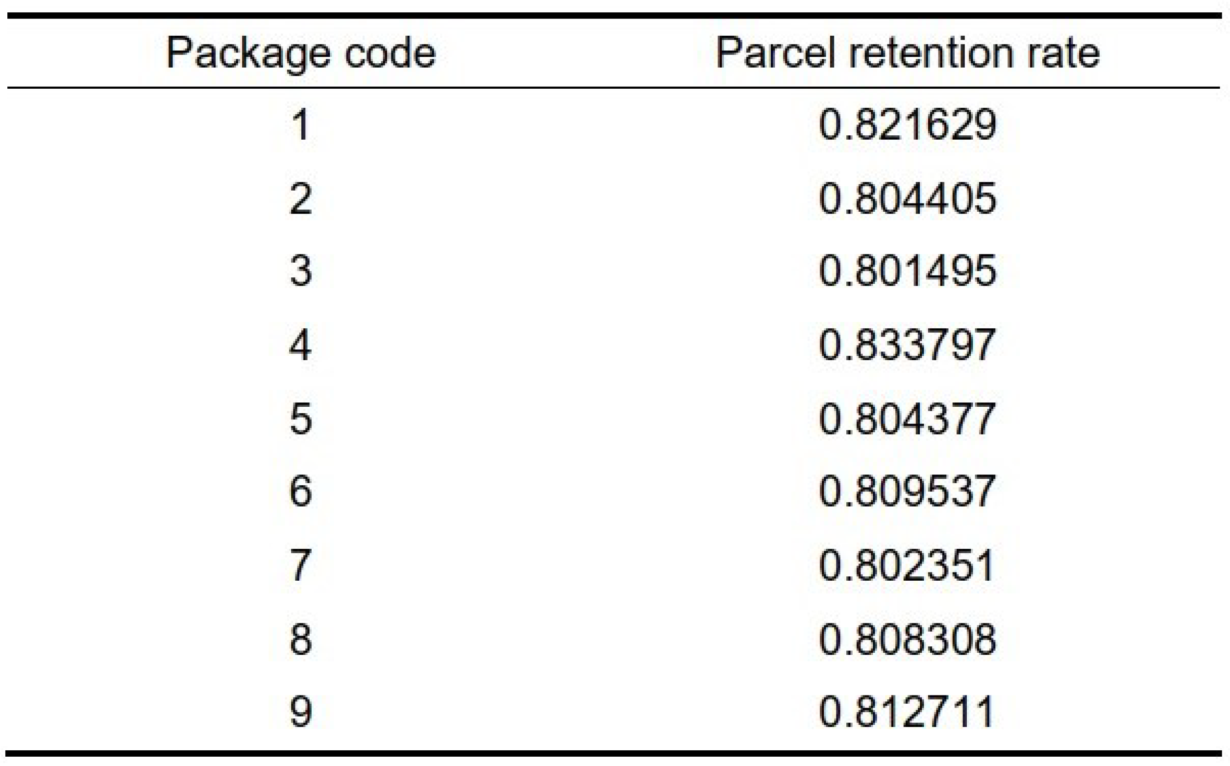
Use Monte Carlo simulation algorithm to obtain the item allocation matrix T for different situations.Through programming software, perform 10000 cycles under restricted conditions. During the cycle, store the maximum value of z in MAX for a single cycle, and use matrix DMAX to store the optimal allocation matrix for the previous several simulation conditions. When there is a value greater than the original DMAX value, replace z * with z and replace DMAX with MAX. After the loop ends, the obtained optimal simulation matrix DMAX is the optimal allocation scheme Y * After calculation, the optimal allocation plan and the parcel shelf life rate is shown in the table below
Table 5. Optimal package calculated shelf life rate.
Preprints 110488 i005

2.11. Conclusion for Model of Task Two

Based on the above analysis, it can be concluded that without considering the time cost of item transportation, the optimal allocation plan that meets the quality assurance rate requirements can be obtained by using the method of single transportation of items by students.

3. Evaluation of the Models

3.1. Evaluation of the Model

3.1.1. Advantages of the Models

(1) The model adopts Monte Carlo simulation algorithm to randomly generate multiple feasible operation plans and compare them pairwise to obtain the optimal plan. This method has a high degree of randomness, and the generated multiple excellent transportation plans can avoid the impact of some students being injured during transportation and unable to transport heavier packages.
(2) The model refers to many widely recognized references within the industry, and has great scientific and practical value.

3.1.2. Disadvantages of the Models

The model adopts Monte Carlo simulation algorithm, which has randomness and may not be able to obtain the best solution within the limited number of times specified by the program. Therefore, it is necessary to run the program repeatedly and verify the results.

3.2. Improvement of the Models

The establishment of the model first drew on numerous widely recognized literature materials in the industry, compared and analyzed them, and then selected the literature that best fits this type of simulation situation for further reference. The established relationship formula has a certain degree of scientific validity and feasibility. Secondly, we used the Monte Carlo simulation algorithm to randomly simulate various situations of transporting student packages and compared them pairwise to obtain the most suitable transportation plan. The random simulation algorithm not only fits the randomness of package allocation to different carriers in real situations, but also avoids the impact of some possible accidents on some carriers. In addition, each model run can provide an equally efficient different transportation plan for selection. The establishment of this model can not only be applied to the logistics transportation industry, but also be extended to all industries involved in the distribution process.

4. Conclusion

In this study, for typical manual freight relocation problem in scenario like college with student labors, we develop integer programming model with minimum transportation time cost target function, with personal load-time cost relationship established incorporating possible shelf life quality constraint. The Monto Carlo simulation algorithm is used to identify the optimized freight allocation scheme with different round trip conditions. The analysis results can be applied to freight relocation scheduling problem for optimal efficiency regarding resource dispatch in educational entities or commercial organizations.

Author Contributions

Conceptualization, Ying Wang and Li Zhao; methodology, Li Zhao; software, Li Zhao and Ying Wang; validation, Ying Wang; formal analysis, Li Zhao; investigation, Ying Wang; resources, Li Zhao and Ying Wang; data curation, Ying Wang; writing—original draft preparation, Li Zhao; writing—review and editing, Li Zhao and Ying Wang; visualization, Ying Wang; supervision, Ying Wang; project administration, Ying Wang; funding acquisition, Ying Wang.

Funding

This research was funded by National Natural Science foundation of China(NSF) under grant number 11547024.

Data Availability Statement

The data of this work cited from references:Weng Jiacheng,Hashemi Ehsan,Arami Arash. Natural Walking With Musculoskeletal Models Using Deep Reinforcement Learning. IEEE ROBOTICS AND AUTOMATION LETTERS,2021,6(2);Seay Joseph F.,Gregory Victoria A.,Frykman Peter N.,Smith Nathaniel I.,Fellin Rebecca E., Spatiotemporal Comparisons Between Male and Female Soldiers While Walking With Heavy Loads:124 Board #5 May 30 9. Medicine & Science in Sports & Exercise,2018,50;Yoganandaan,V. Perumalm Effect of Walking with and without LoadIntermittent Walking on Cardio Respiratory Endurance Muscular Strength and Muscular Endurance of Adolescent Boys. International Journal of Innovative Research and Development,2014,3(13)

Conflicts of Interest

The authors declare no conflicts of interest.

Appendix A. Student-Item Sample Data (For Test in This Work)
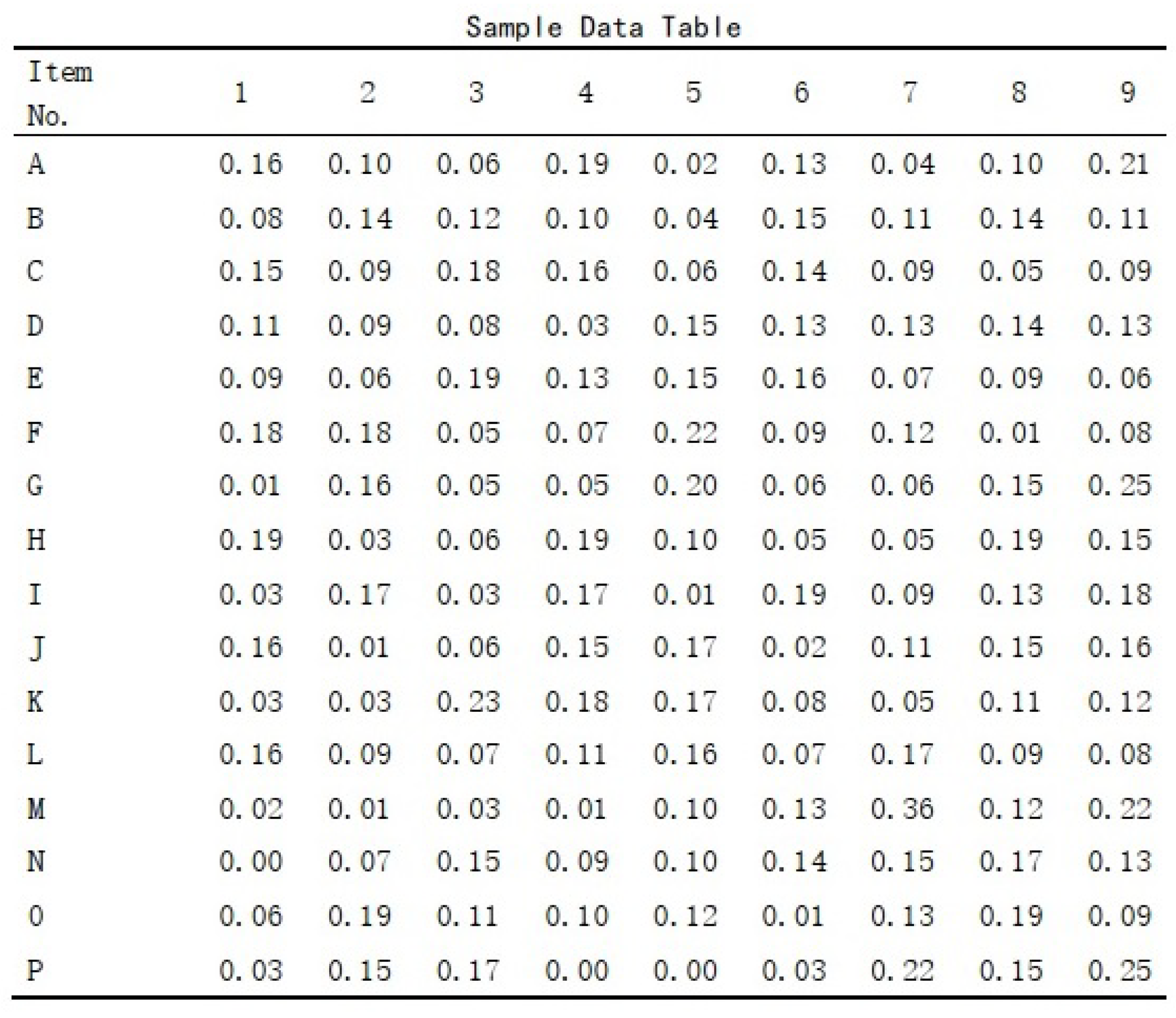
Figure A1. Student-Load Data (for 9 students, data in unit of 30kg).
Preprints 110488 g0a1

Appendix B. Matlab Code

SS=0;SS1=0;SS2=0; SS3=0;SS4=0;
kongvalue1=5;
kongvalue2=6;
kongvalue3=7;
SSmin=10000;
TRSSN=zeroSS(3,9);
trSSn=zeroSS(3,9);
for timeSS=1:2000 for i=1:2 tr1=randi([2,10]);
tr2=randi([2,10]);
tr3=randi([2,10]);
tr4=randi([4,12]);
tr5=randi([4,12]);
tr6=randi([4,12]);
tr7=randi([6,16]);
tr8=randi([6,16]);
tr9=randi([6,16]);
TRSSN(i,:)=[tr1,tr2,tr3,tr4,tr5,tr6,tr7,tr8,tr9];
SymS vv1;
SymS v2;
SymS v3;
SymS v4;
SymS v5;
SymS v6;
SymS v7;
SymS v8;
SymS v9;
[vv1]=vpaSolve([(3.9638/(1-vv1))/2.0736==1.5+2*(1+tr1/2.0736)*(tr1/2.0736)*(tr1/2.0736)+1.5*vv1*vv1* (1+tr1/2.0736)],[vv1]);
[v2]=vpaSolve([(3.6729/(1-v2))/1.9214==1.5+2*(1+tr2/1.9214)*(tr2/1.9214)*(tr2/1.9214)+1.5*v2*v2* (1+tr2/1.9214)],[v2]);
[v3]=vpaSolve([(3.4442/(1-v3))/1.8018==1.5+2*(1+tr3/1.8018)*(tr3/1.8018)*(tr3/1.8018)+1.5*v3*v3* (1+tr3/1.8018)],[v3]);
[v4]=vpaSolve([(8.2578/(1-v4))/3.5795==1.5+2*(1+tr4/3.5795)*(tr4/3.5795)*(tr4/3.5795)+1.5*v4*v4* (1+tr4/3.5795)],[v4]);
[v5]=vpaSolve([(8.0229/(1-v5))/3.4777==1.5+2*(1+tr5/3.4777)*(tr5/3.4777)*(tr5/3.4777)+1.5*v5*v5* (1+tr5/3.4777)],[v5]);
[v6]=vpaSolve([(7.5248/(1-v6))/3.2617==1.5+2*(1+tr6/3.2617)*(tr6/3.2617)*(tr6/3.2617)+1.5*v6*v6* (1+tr6/3.2617)],[v6]);
[v7]=vpaSolve([(13.7822/(1-v7))/5.1146==1.5+2*(1+tr7/5.1146)*(tr7/5.1146)*(tr7/5.1146)+1.5*v7*v7* (1+tr7/5.1146)],[v7]);
[v8]=vpaSolve([(12.9585/(1-v8))/4.8089==1.5+2*(1+tr8/4.8089)*(tr8/4.8089)*(tr8/4.8089)+1.5*v8*v8* (1+tr8/4.8089)],[v8]);
[v9]=vpaSolve([(12.1348/(1-v9))/4.5032==1.5+2*(1+tr9/4.5032)*(tr9/4.5032)*(tr9/4.5032)+1.5*v9*v9* (1+tr9/4.5032)],[v9]);
vv1=real(vv1(1,1));
v2=real(v2(1,1));
v3=real(v3(1,1));
v4=real(v4(1,1));
v5=real(v5(1,1));
v6=real(v6(1,1));
v7=real(v7(1,1));
v8=real(v8(1,1));
v9=real(v9(1,1));
T1=1/vv1;
T2=1/v2;
T3=1/v3;
T4=1/v4;
T5=1/v5;
T6=1/v6;
T7=1/v7;
T8=1/v8;
T9=1/v9;
SS2=T1+T2+T3+T4+T5+T6+T7+T8+T9+kongvalue1*3+kongvalue2*3+kongvalue3*3;
SS1=SS2+SS1;
clear vv1;
clear v2;
clear v3;
clear v4;
clear v5;
clear v6;
clear v7;
clear v8;
clear v9;
SS=tr1+tr2+tr3+tr4+tr5+tr6+tr7+tr8+tr9;
SS3=SS+SS3;
if SS3>=197 break end
end
for j=1:100 SS4=SS3;
tr1=randi([2,10]);
tr2=randi([2,10]);
tr3=randi([2,10]);
tr4=randi([4,12]);
tr5=randi([4,12]);
tr6=randi([4,12]);
tr7=randi([6,16]);
tr8=randi([6,16]);
tr9=randi([6,16]);
ifnot=round(rand(1,9));
tr1=tr1*ifnot(1,1);
tr2=tr2*ifnot(1,2);
tr3=tr3*ifnot(1,3);
tr4=tr4*ifnot(1,4);
tr5=tr5*ifnot(1,5);
tr6=tr6*ifnot(1,6);
tr7=tr7*ifnot(1,7);
tr8=tr8*ifnot(1,8);
tr9=tr9*ifnot(1,9);
SS=tr1+tr2+tr3+tr4+tr5+tr6+tr7+tr8+tr9;
SS4=SS4+SS;
if SS4<197 continue end
TRSSN(3,:)=[tr1,tr2,tr3,tr4,tr5,tr6,tr7,tr8,tr9];
SymS vv1;
SymS v2;
SymS v3;
SymS v4;
SymS v5;
SymS v6;
SymS v7;
SymS v8;
SymS v9;
[vv1]=vpaSolve([(3.9638/(1-vv1))/2.0736==1.5+2*(1+tr1/2.0736)*(tr1/2.0736)*(tr1/2.0736)+1.5*vv1*vv1* (1+tr1/2.0736)],[vv1]);
[v2]=vpaSolve([(3.6729/(1-v2))/1.9214==1.5+2*(1+tr2/1.9214)*(tr2/1.9214)*(tr2/1.9214)+1.5*v2*v2* (1+tr2/1.9214)],[v2]);
[v3]=vpaSolve([(3.4442/(1-v3))/1.8018==1.5+2*(1+tr3/1.8018)*(tr3/1.8018)*(tr3/1.8018)+1.5*v3*v3* (1+tr3/1.8018)],[v3]);
[v4]=vpaSolve([(8.2578/(1-v4))/3.5795==1.5+2*(1+tr4/3.5795)*(tr4/3.5795)*(tr4/3.5795)+1.5*v4*v4* (1+tr4/3.5795)],[v4]);
[v5]=vpaSolve([(8.0229/(1-v5))/3.4777==1.5+2*(1+tr5/3.4777)*(tr5/3.4777)*(tr5/3.4777)+1.5*v5*v5* (1+tr5/3.4777)],[v5]);
[v6]=vpaSolve([(7.5248/(1-v6))/3.2617==1.5+2*(1+tr6/3.2617)*(tr6/3.2617)*(tr6/3.2617)+1.5*v6*v6* (1+tr6/3.2617)],[v6]);
[v7]=vpaSolve([(13.7822/(1-v7))/5.1146==1.5+2*(1+tr7/5.1146)*(tr7/5.1146)*(tr7/5.1146)+1.5*v7*v7* (1+tr7/5.1146)],[v7]);
[v8]=vpaSolve([(12.9585/(1-v8))/4.8089==1.5+2*(1+tr8/4.8089)*(tr8/4.8089)*(tr8/4.8089)+1.5*v8*v8* (1+tr8/4.8089)],[v8]);
[v9]=vpaSolve([(12.1348/(1-v9))/4.5032==1.5+2*(1+tr9/4.5032)*(tr9/4.5032)*(tr9/4.5032)+1.5*v9*v9* (1+tr9/4.5032)],[v9]);
vv1=real(vv1(1,1));
v2=real(v2(1,1));
v3=real(v3(1,1));
v4=real(v4(1,1));
v5=real(v5(1,1));
v6=real(v6(1,1));
v7=real(v7(1,1));
v8=real(v8(1,1));
v9=real(v9(1,1));
T1=1/vv1;
T2=1/v2;
T3=1/v3;
T4=1/v4;
T5=1/v5;
T6=1/v6;
T7=1/v7;
T8=1/v8;
T9=1/v9;
SS2=T1+T2+T3+T4+T5+T6+T7+T8+T9+ifnot(1,1)*kongvalue1+ifnot(1,2)*kongvalue1+ifnot(1,3)* kongvalue1+ifnot(1,4)*kongvalue2+ifnot(1,5)*kongvalue2+ifnot(1,6)*kongvalue2+ifnot(1,7) *kongvalue3+ifnot(1,8)*kongvalue3+ifnot(1,9)*kongvalue3;
SS1=SS2+SS1;
clear vv1;
clear v2;
clear v3;
clear v4;
clear v5;
clear v6;
clear v7;
clear v8;
clear v9;
if SS1<SSmin SSmin=SS1;
trSSn=TRSSN;
end
if SS4>197 break end end end

References

  1. Bertsch, C.; Unger, H.; Winkelmann, W.; et al. Evaluation of early walking patterns from plantar pressure distribution measurements. Gait Posture 2004, 19(3), 235–242. [Google Scholar] [CrossRef] [PubMed]
  2. Eleftherios, K. Plantar pressure distribution during barefoot standing, walking and landing in preschool boys. Gait Posture 2001, 14, 92–97. [Google Scholar]
  3. Willems, T.; Witvrouw, E.; Itvrouw, E.; Delbaere, K.; et al. Relationship between gait biomechanics and inversion sprains: a prospective study of risk factors. Gait Posture 2005, 21, 379–387. [Google Scholar] [CrossRef]
  4. Dixon, P.C.; Stebbins, J.; Theologis, T.; et al. Spatio-temporal parameters and lower -limb kinematics of turning gait in typically developing children. Gait and Posture 2013, 38, 870–875. [Google Scholar] [CrossRef] [PubMed]
  5. Kerrigan, D.C.; Riley, P.O.; Nieto, T.J.; et al. Knee joint torques: a comparison between women and men during barefoot walking. Archives of Physical Medicine and Rehabilitation 2000, 81, 1162–1165. [Google Scholar] [CrossRef] [PubMed]
  6. Wang, Y.; Pascoe, D.D.; Weimar, W. Evaluation of book back-pack load during walking. Ergonomics 2001, 44, 858–869. [Google Scholar] [CrossRef] [PubMed]
  7. Goh, J.H.; Thambyah, A.; Bose, K. Effects of varying backpackloads on peak forces in the lumbosacral spine during walking[J]. Clinical Biomechanics 1998, 13(1- supp -S1), s26–s31. [Google Scholar] [CrossRef]
  8. Castro, M.P.; Figueiredo, M.C.; Abreu, S.; et al. The influenceof gait cadence on the ground reaction forces and plantar pressuresduring load cariage of young adults. Applied Ergonomics 2015, 49, 41–46. [Google Scholar] [CrossRef]
  9. Stergiou, N.; Moraiti, C.; Giakas, G.; et al. The effect of the walking speed on the stability of the anterior cruciate ligament deficient knee. ClinBiomech 2004, 19, 957–963. [Google Scholar] [CrossRef] [PubMed]
  10. Grieve, D.W.; Gear, R.J. The relationship between length of stride,step requency,time ofswing,and speed of walking for children and adults. Ergonomics 1966, 5, 379–399. [Google Scholar] [CrossRef] [PubMed]
  11. Bobet,J.; and Norman, R.W. Effects of load placement on back muscle activity in loadcarriage. Eur.J Appl physiol 1984, 53, 71–75. [CrossRef] [PubMed]
  12. Weng, J.C.; Hashemi, E.; Arami, A. Natural Walking With Musculoskeletal Models Using Deep Reinforcement Learning. IEEE ROBOTICS AND AUTOMATION LETTERS 2021, 6. [Google Scholar] [CrossRef]
  13. Ji, Q.; Fu, S.; Tan, K.; Muralidharan, S.T.; Lagrelius, K.; Danelia, D.; et al. Synthesizing the optimal gait of a quadruped robot with soft actuators using deep reinforcement learning. Robotics and Computer Integrated Manufacturing: An International Journal of Manufacturing and Product and Process Development 2022. [Google Scholar] [CrossRef]
  14. Mishra, U. A. Learning Control Policies for Imitating Human Gaits. 2021. [Google Scholar] [CrossRef]
  15. Seay, J.F.; Gregory, V.A.; Frykman, P.N.; Smith, N.I.; Fellin, R.E. Spatiotemporal Comparisons Between Male and Female Soldiers While Walking With Heavy Loads:124 Board #5 May 30 9. Medicine & Science in Sports & Exercise, 2018, 50. [Google Scholar]
  16. Simpkins, C.; Yang, F. Dynamic Gait Stability and Spatiotemporal Gait Parameters During Overground Walking in Professional Ballet Dancers[J]. Journal of dance medicine & science 2024, 28. [Google Scholar]
  17. Seay, J.F.; Bode, V.G.; Frykman, P.N.; et al. Pelvis and Trunk Motion Comparisons Between Male and Female Soldiers While Walking With Heavy Loads: 85 Board #1 May 29 9:30 AM - 11:30 AM[J]. Medicine & Science in Sports & Exercise 2019, 51. [Google Scholar] [CrossRef]
  18. Simpson, K.M.; Munro, B.J.; Steele, J.R. Effects of prolonged load carriage on ground reaction forces, lower limb kinematics and spatio-temporal parameters in female recreational hikers[J]. Ergonomics 2012, 55, 316–326. [Google Scholar] [CrossRef] [PubMed]
  19. Houck, J.R.; Duncan, A.; Haven, K.E.D. Comparison of frontal plane trunk kinematics and hip and knee moments during anticipated and unanticipated walking and side step cutting tasks[J]. Gait & Posture 2006, 24, 314–322. [Google Scholar] [CrossRef]
  20. S. Yoganandaan,V. P. Effect of Walking with and without LoadIntermittent Walking on Cardio Respiratory EnduranceMuscular Strength and Muscular Endurance of Adolescent Boys[J]. International Journal of Innovative Research and Development 2014, 3.
  21. Lee, J.S.; et al. Effects of Forest-Walking Exercise on Isokinetic Muscular Strength, Muscular Endurance, and Bone Mineral Density in the Elderly Women[J]. Journal of the Korean Institute of Forest Recreation 2016, 20, 1–9. [Google Scholar] [CrossRef]
  22. Wernbom, M.; et al. EFFECTS OF VASCULAR OCCLUSION ON MUSCULAR ENDURANCE IN DYNAMIC KNEE EXTENSION EXERCISE AT DIFFERENT SUBMAXIMAL LOADS. Journal of Strength & Conditioning Research 2006. [Google Scholar]
  23. Harrison, P.W.; James, L.P.; Jenkins, D.G.; et al. The Effects of Low-Load Squat Jump and Maximal Isometric Priming Exercise on Muscular Performance and Perceptual State[J]. Journal of strength and conditioning research 2024, 38. [Google Scholar] [CrossRef] [PubMed]
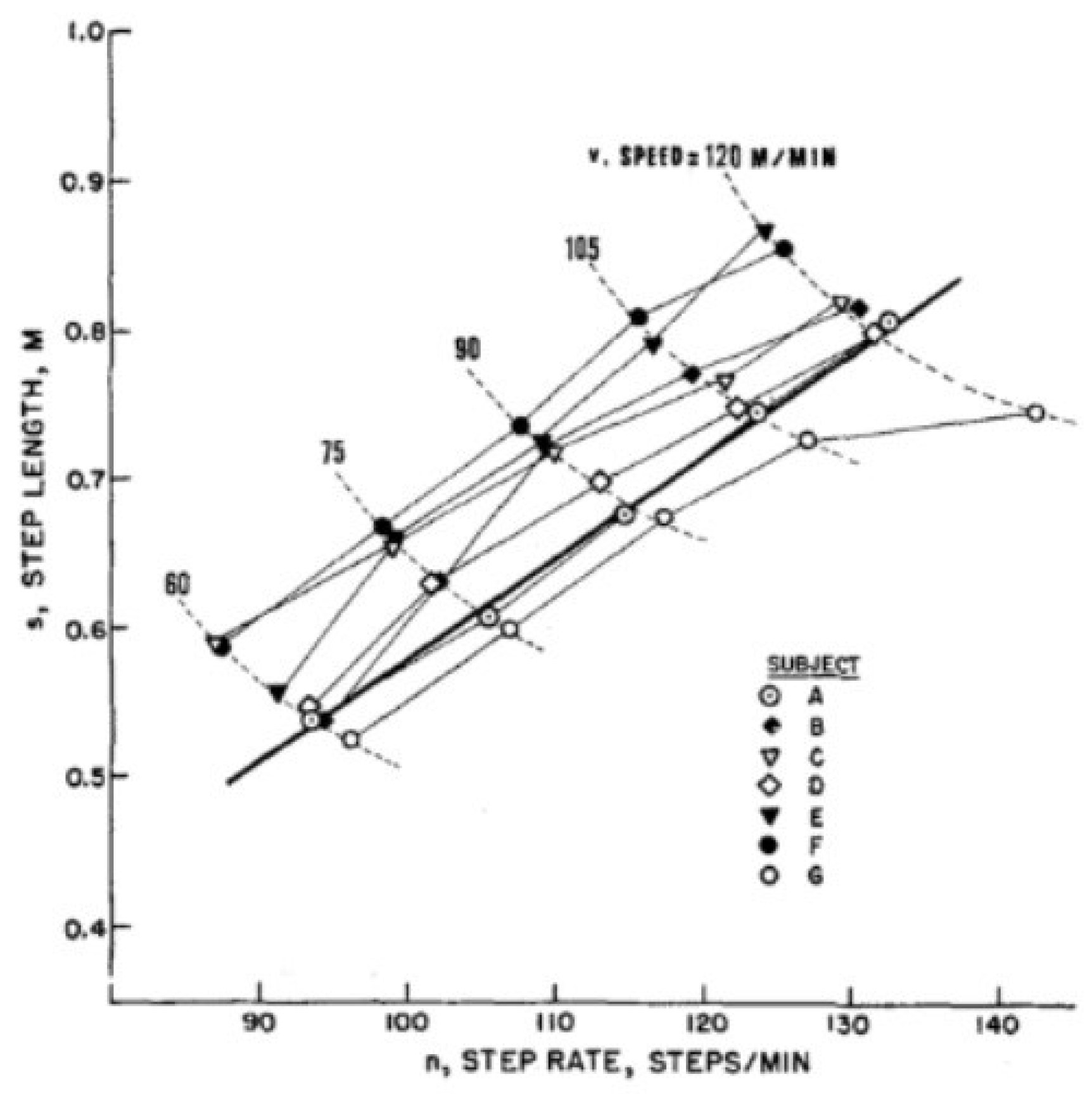
Figure 1. Model of freely selecting step size under variable speed.
Preprints 110488 g001
Figure 2. Relationship between oxygen consumption and load during flat ground load carrying travel.
Preprints 110488 g002
Disclaimer/Publisher’s Note: The statements, opinions and data contained in all publications are solely those of the individual author(s) and contributor(s) and not of MDPI and/or the editor(s). MDPI and/or the editor(s) disclaim responsibility for any injury to people or property resulting from any ideas, methods, instructions or products referred to in the content.
Copyright: This open access article is published under a Creative Commons CC BY 4.0 license, which permit the free download, distribution, and reuse, provided that the author and preprint are cited in any reuse.
Prerpints.org logo

Preprints.org is a free preprint server supported by MDPI in Basel, Switzerland.

Subscribe

© 2024 MDPI (Basel, Switzerland) unless otherwise stated