1. Introduction
Visualization of volumetric data is an important discipline, especially in medical and biomedical applications [
1]. Various image acquisition techniques, such as fMRI or 3D microscopy, are used to generate volumetric data. In addition to their use in everyday medical practice for the preparation and follow-up of surgical interventions, visualizations are also used for teaching purposes: in publications, textbooks, or for understanding one’s own research results. Beyond displaying single images, atlases can be created using imaging techniques, as in the case of the zebrafish larval brains [
2] or for whole brain MRI [
3]. Thus, various tools have been developed by which the rendering can be performed. Prominent tools in research are 3D Slicer [
4] and Fiji [
5] including plugins for visualization such as ClearVolume [
6]. Beyond that, Matlab is a prominent platform for 3D image analysis within the scientific community [
7,
8]. Several extensions and modules were created, such as VoxelStats [
9] which offers tooling for voxel wise brain analysis. Another package is Hydra image processor [
10], which forms a GPU image analysis library with MATLAB and Python wrapper. Beyond that, dedicated rendering capabilities are offered by Matlab itself in their Volume Viewer App [
11] as well as by the community projects VolumeRender [
12] and Ray Tracing Volume Renderer [
13]. However, although these tools usually come with some visualization functionality or are specifically designed for this purpose, a complete controllable rendering functionality and supporting light sources is not featured. Further, rendering of volumetric data is computational demanding, especially as technology advances and volumetric data increase in size. However, this can be accelerated with the latest graphics hardware. While a very expensive step using GPUs is the data transfer from host to device [
14], a memory management reducing these transactions formed a requirement.
To address the current limitations of existing solutions, we present in this work a novel GPU-accelerated rendering system that features fully adjustable emission, absorption, and reflection properties, along with a configurable illumination setup. Our system allows modification of camera parameters to create animations and stereo images for 3D displays. In order to realize this while guaranteeing high usability to the end user, a MATLAB® interface was created interfacing to the renderer process which itself was implemented in C++ and CUDA. These capabilities enable the creation of complex, high-quality renderings while taking advantage of the speed of modern GPUs, allowing scientists to use MATLAB® as a comprehensive tool for analysis and visualization, thereby streamlining workflows within a single environment.
1.1. Rendering Equation
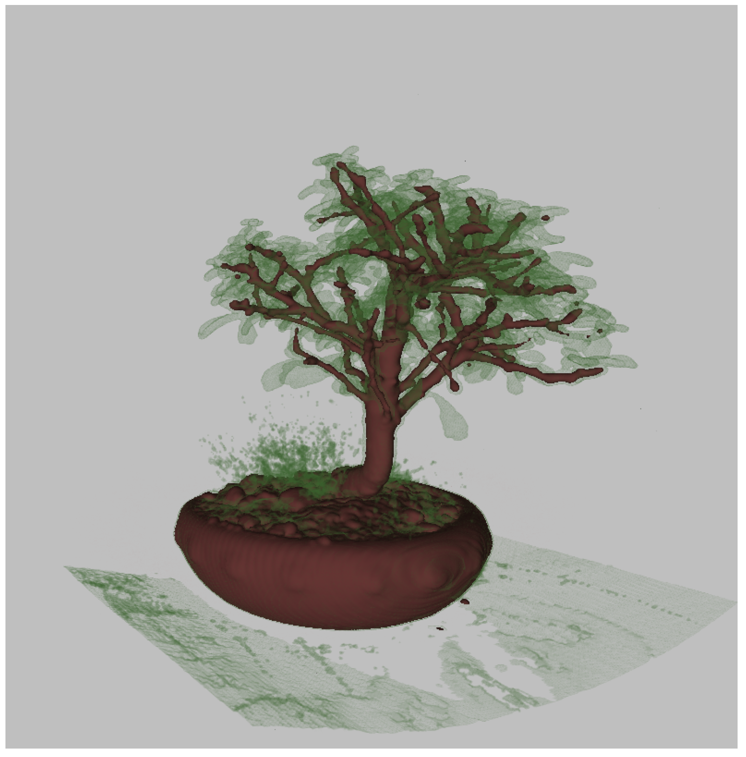
There are two methods to render a volume: indirect and direct volume rendering (see
Figure 1). Indirect rendering is used to render the isosurface of a volume [16]. First the generation of an intermediate representation of the data set is required (e.g. a polygonal representation of an isosurface generated by Marching Cubes [17]). The second step is the rendering of this representation. In a polygonal representation only a limited number of the 3D data set directly contributes to the 2D output. The interior of the volume is not considered.
Figure 1.
This illustration shows a CT scan of a bonsai. The leafs are visualized by direct volume rendering whereas the trunk and the branches are visualized using an isosurface rendering. Obviously in the direct volume rendering each voxel contributes to the resulting 2D image. (image source: [
15]).
Since in biological or medical application the interior is of utmost importance, for our application we use direct rendering [18]. Direct rendering techniques do not need the generation of an intermediate representation of the data set, since every voxel contributes to the resulting 2D image. To abide to core physical properties of the rendering process, we use a model that takes emission and absorption into account. In this model every particle emits and absorbs light. The combination of all these properties is maintained in the following rendering equation, a simplified version of the equation introduced by [19]:
This equation integrates from 0, the edge of the volume, to D at the eye. describes the value of accumulated light intensity of one ray traversing the volume. is the absorption at t and is the sampled value at s.
In fact, the equation consists of two main terms: denotes emission and the transparency at point s.
1.1.1. Emission
In general, the emission part of the used model described in Eq. 1 assumes that each particle of the volume denotes a tiny light source. Thus, even if no external light source is applied, the volume can emit a certain amount of light. This behavior is motivated by the following applications:
-
Microscopy
- (a)
Self-luminous particles are modelled. This occurs during fluorescence microscopy, as certain proteins glow.
- (b)
The particle is illuminated by a light source. This leads to a better spatial impression.
-
MRI
- (a)
Magnetic signals are processed. Varying values are transformed into visual signals.
- (b)
No external illumination is applied/applicable while recording data. However, in a voxel grid, the signals can be compared to self-illuminated particles.
In the used model this light is not scattered. What is more, we neglect the attenuation of light on the path from the light source to an enlightened particle and we neglect the attenuation of light from the volume to the camera as well. This is not completely physically correct but enables a simple model and thus a high computational performance.
Figure 2 illustrates this simplification.
1.1.2. Absorption
In our case absorption describes the attenuation of light. Eq. 2 describes the transparency between point
s and the eye. If we assume a transparency of
we can simply reformulate this transparency such that it becomes opacity by
.
1.1.3. Discretization
Since Eq. 1 cannot be solved analytically for all interpolation methods, to obtain a general discretization one has to solve it numerically. This can be easily done by the Riemann sum and a fixed step size
. The step size scales the current sampling position along the ray. More precisely, the ray gets divided into
n equal segments, each of size
[19].
Thus, we end up with the discretized rendering equation that approximates Eq. 1:
2. Material and Methods
2.1. Rendering Pipeline
The rendering pipeline defines the order of the operations that are processed to compute the discretized rendering equation.
Our renderer uses the three operations sampling, illumination and compositing that are explained more precisely in the following sections.
2.1.1. Sampling
As already described, the ray is divided into n equal segments. This transformation of a continuous ray to discretized volume intersection locations is called sampling. To perform good quality, the discretized ray positions are interpolated. What is more, in order to avoid artifacts, the sampling rate should be twice as high as the grid resolution [21].
Each image pixel is computed by one ray. A ray passes through the center of its corresponding pixel.
2.1.2. Illumination
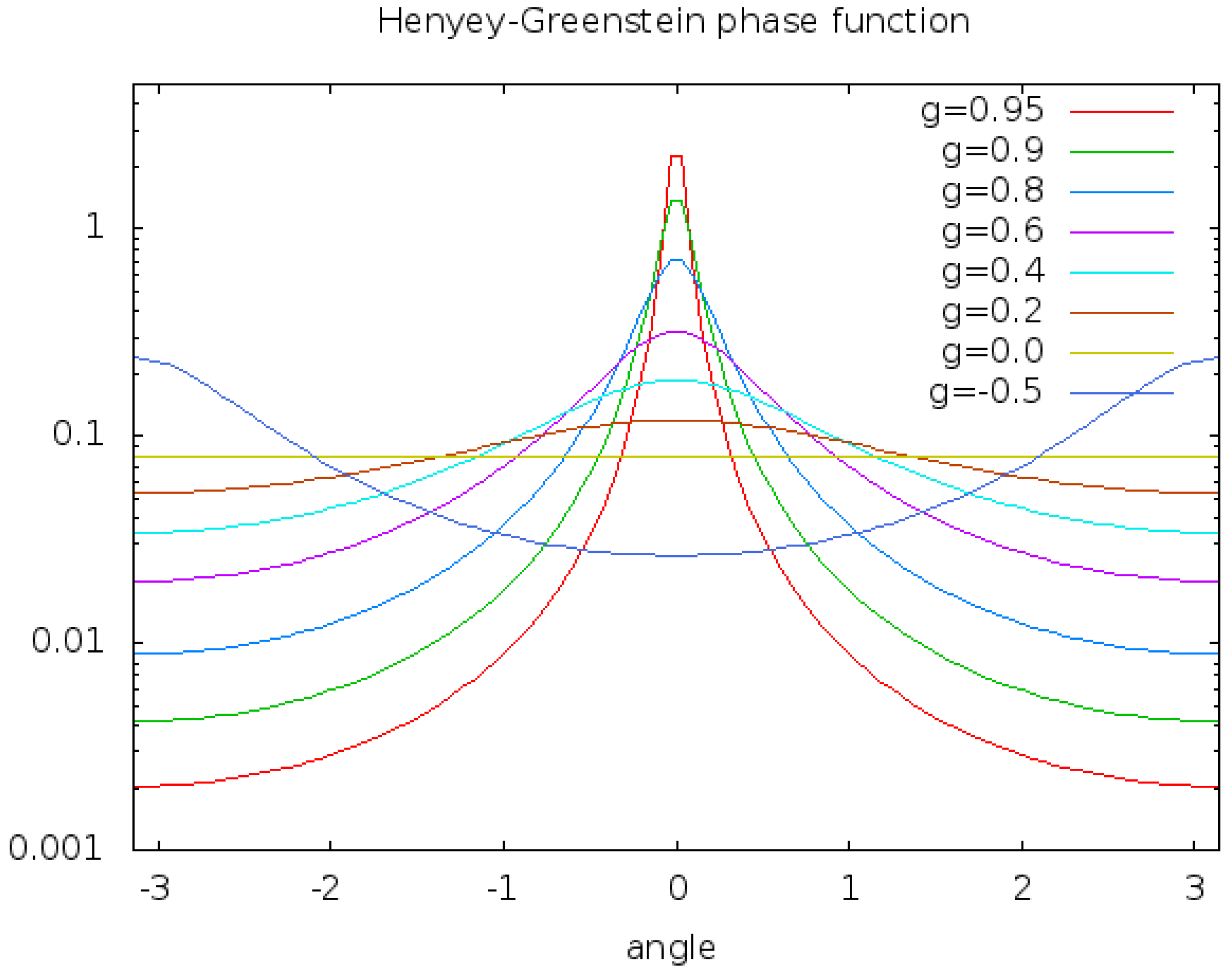
To improve the realism of the rendered scene our renderer provides an interface for local illumination techniques. For our application of microscopy, we decided to use the Henyey-Greenstein phase function [22].
where
g characterizes the distribution and
the angle.
HG behaves physically more correct than other shading functions like e.g. Blinn-Phong [23] while being computationally inexpensive.
Figure 3 depicts the function for several
g.
At each sample position this function is evaluated locally. This illumination model ignores scattering as well as diffusion. Any interaction with other particles is neglected and the light arrives unextenuated at the sample point.
2.1.3. Compositing
Compositing denotes the accumulation of the sampled, illuminated and colored values along the ray to a coherent result. Therefore, in this case we use the discretized rendering equation we explained in the previous section.
One can reformulate Eq. 4 and use the basic compositing
over-operator introduced by [24]:
Since our samples are sorted in front-to-back order our renderer uses the
under-operator. Combined with alpha compositing this yields to the following equations [25]:
where
and
denotes the accumulated color including the illumination and opacity as described in
Section 1.1.2. Besides front-to-back compositing has the advantage, that the ray can be stopped if a given threshold (of transparency) is reached.
2.2. Stereo Rendering
There are many possibilities for a stereo rendering setup. Some of these approaches do not produce correct results.
Toe-in is easy to implement. Since in this projection the two stereo cameras are pointing to the same focal point, a rotation of the object suffices to render the two images. Unfortunately, one suffers from vertical parallax. The higher the distance to the center of the projection plane, the more this effect occurs. Thus this approach does not result in correct stereo images.
Figure 4 illustrates this rendering setup.
2.2.1. Off-Axis
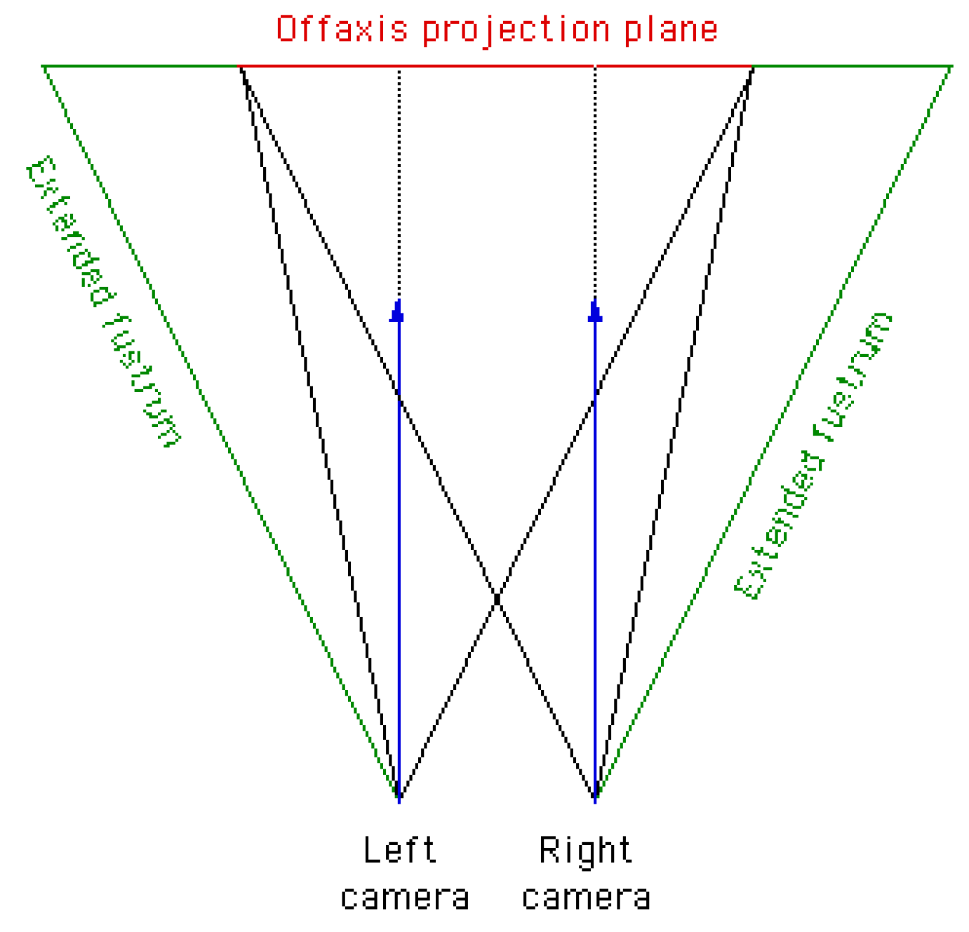
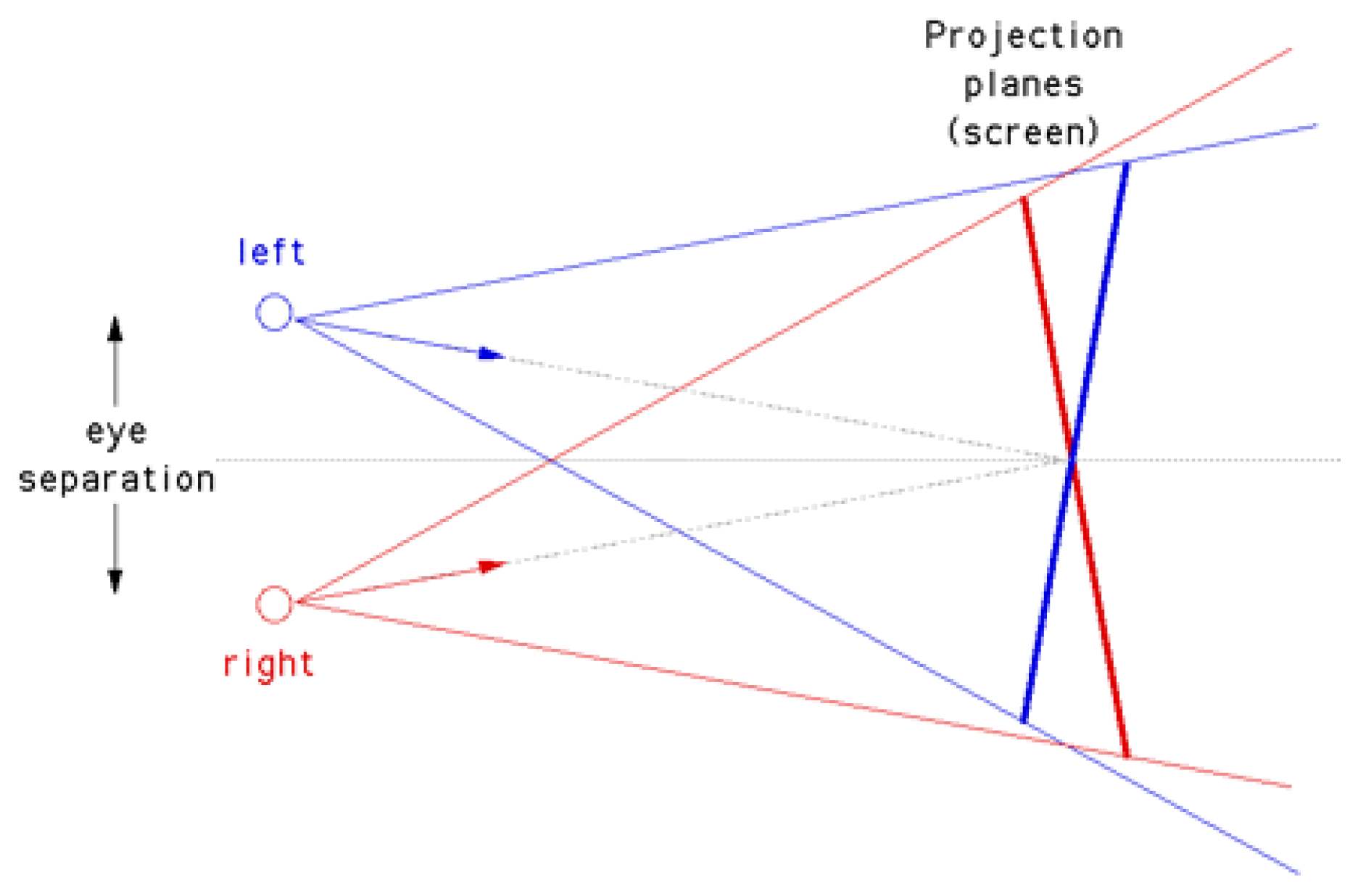
Off-axis is the correct projection. No vertical parallax is introduced. Both cameras have a different focal point (see
Figure 5). The viewing directions are parallel. Thus, it is necessary to render two images with different camera view frustums. However, the two extended camera frustums do not overlap completely. To obtain the off-axis projection plane of both images, one has to trim the projection of the extended frustums. Therefore, one has to compute the non-overlapping amount of pixels
[26]:
where
w is the image width in pixel and
is the focal length.
b is the stereo base, i.e. half of camera x-offset. The angle of view
can be computed as follows:
where
d is the width of the normalized image plane. In our case
because the range of the normalized image plain goes from -1 to 1.
If now a stereo image of resolution is rendered, first this resolution will be extended by . Then the left and right images with a resolution of are rendered. Finally, to obtain the off-axis projection plane both images are trimmed respectively to again.
Figure 5.
The correct off-axis stereo camera setup. The extended frustums are depicted. To obtain the off-axis projection plane one has to trim the projection plane of each extended frustum (image source: [26]).
Figure 5.
The correct off-axis stereo camera setup. The extended frustums are depicted. To obtain the off-axis projection plane one has to trim the projection plane of each extended frustum (image source: [26]).
2.3. Implementation
2.3.1. Architecture
To obtain a high computational performance we decided to use the NVIDIA CUDA toolkit as it provides an interface for highly parallelized computation on GPU. Since CUDA is only available for NVIDIA devices, we are restricted in the choice of the graphic card. Moreover, the renderer was developed using MATLAB® 2023a relying on CUDA 10.2 which needs compatible devices.
CUDA provides a special CUDA-C compiler. This GPU device code can easily be connected to the host (CPU) C++ code. The host code provides some data structures and functions that handle the communication between host and device. Using the MATLAB® mex-interface we built a MATLAB® command. For this purpose, MATLAB® provides a special compiler, that translates all the compiled C object files into a MATLAB® command. As the MATLAB® renderer command requires a lot of parameters we developed some wrapper classes with special properties to make the handling more comfortable. Compilation is straightforward, performed inside MATLAB using make.m, mex, and mexcuda. Users only need to set up a compatible compiler and install CUDA, following the provided instructions.
2.3.2. Ray Casting
Ray casting describes the process of shooting rays starting from the viewer/camera through the volume. If a ray intersects the volume, an accumulated light intensity is determined while traversing the volume. For each ray a test is performed if it intersects the volume. As we only provide the opportunity to render one object per rendering pass, this test is only performed once for each ray. As [27] introduces a fast intersection test approach that also performs well if there is only one intersection per ray, we decided to implement a slightly simplified version of this algorithm. In our case of only one intersection test per ray we omitted complex data structures.
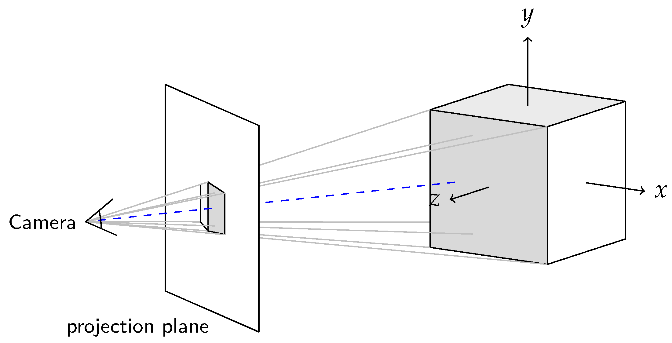
Moreover, we defined the origin of the world coordinate frame in the middle of the volume. A scalar
d describes the distance to the volume. Through this, the camera is moved along the negative z-axis to its position. The distance between projection plane and camera is defined to 1. What is more, the focal length
can be customized. With a rotation matrix
R we can now rotate the camera around the object.
Figure 6 depicts such a example scene.
The projection plane is defined in normalized coordinates from to . Each rendered pixel value is determined by one ray. Thus, we have to project the respective x and y coordinate of the ray to the normalized projection plane coordinates u and v.
With all these information, we can compute the direction of a ray and its position with
,
and
are the particular column vectors of the rotation matrix.
is the camera x-offset that can be defined by the user.
Since we are computing on the GPU each ray, representing one pixel of the rendered image, was computed by one CUDA thread. Thus, we obtained a highly parallelized rendering program.
2.3.3. Memory Management
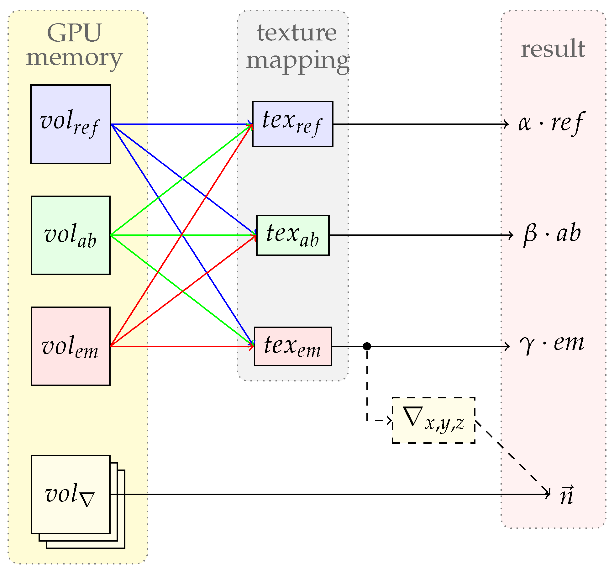
GPU memory is very limited and not extendable. Usually our renderer requires six different volumes: one for emission, one for absorption, one for reflection and one for each gradient direction. If all these volumes are copied to the GPU this might lead to a high memory consumption. In some cases these volumes can be similar or they differ only by a scalar factor. E.g. one can have an emission volume
and an absorption volume
. Due to the texture mapping
NVIDIA CUDA provides to perform efficient lookups, it is possible to map one volume to multiple textures [28]. This enables us to map
to
. To provide the possibility that the looked up value is multiplied by a scalar factor, the renderer is enabled to setup one scalar multiplicator for the emission, absorption and reflection volume. To be able to save more GPU memory one can setup the renderer to compute the gradient on the fly. As expected this is computationally more expensive, especially if a movie sequence of one scene is rendered.
Figure 7 shows the possible options.
The illumination volume and the light sources are copied to the GPU memory as well. Volumes are only copied to the device if they have been modified since the last rendering process. This minimizes the host to GPU transactions and increases the rendering performance of scenes with multiple images.
2.3.4. Illumination Model Interface
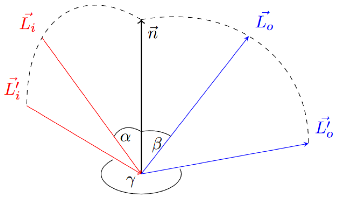
In order to provide a some degree of freedom for the illumination model, we used a 3D lookup table. The lookup table describes the interaction of a particle with a light source as depicted in
Figure 8. Since we know where the light source and the view point are located, the vector of the incoming light
and the vector of the outgoing light
are known.
equals the view direction. The normal vector
is approximated by the negative gradient. As described in
Section 2.3.3 the gradient is either determined by
or computed on the fly using the finite difference scheme. With this information
and
can be computed.
is the angle between
and
, the projections of
and
onto the surface plane. We can compute these projected vectors as follows:
where
is the position of the light source and
is the
is the view point.
After the calculation of these angles the light intensity can be established by performing a lookup. Since the LUT contains only a finite number of entries, linear interpolation is applied. The underlying LUT can be built up with a lot of illumination models. In the next section we present how we built such a LUT for the HG phase function.
2.3.5. Henyey-Greenstein
Our renderer uses the Henyey-Greenstein phase function to compute the light intensity (see Eq. 5). The corresponding LUT is built up with the angles
,
and
. Unfortunately,
is the angle between
and
. Thus we had to compute
for each
,
and
. In order to compute the LUT we chose
while
and
were iterated respectively dependent on the resolution of the LUT. To perform the rotation around the surface normal we build a rotation matrix
around the surface normal dependent on
. Because of the properties of the unit circle that we are working with, the rotation matrix is around the x-axis.
is kept fix while
is rotated. Now
is computed by using the dot-product:
Because the three angles are iterated, we end up in a three time nested loop. To obtain high performance we decided to implement the computation of the LUT in C++ and and provide API bindings to MATLAB®. Thus we provide a fast computation of this LUT via a MATLAB® command. The parameters are the resolution of the LUT and g (see Eq. 5). As mentioned before, the LUT contains only a finite number of entries. Thus, during a lookup a linear interpolation is applied.
2.4. MATLAB ® Interface
The compiled MATLAB® command of the volume renderer exposes several input parameters. Thus, we decided to write complementary wrapper classes to further simplify the developer experience.
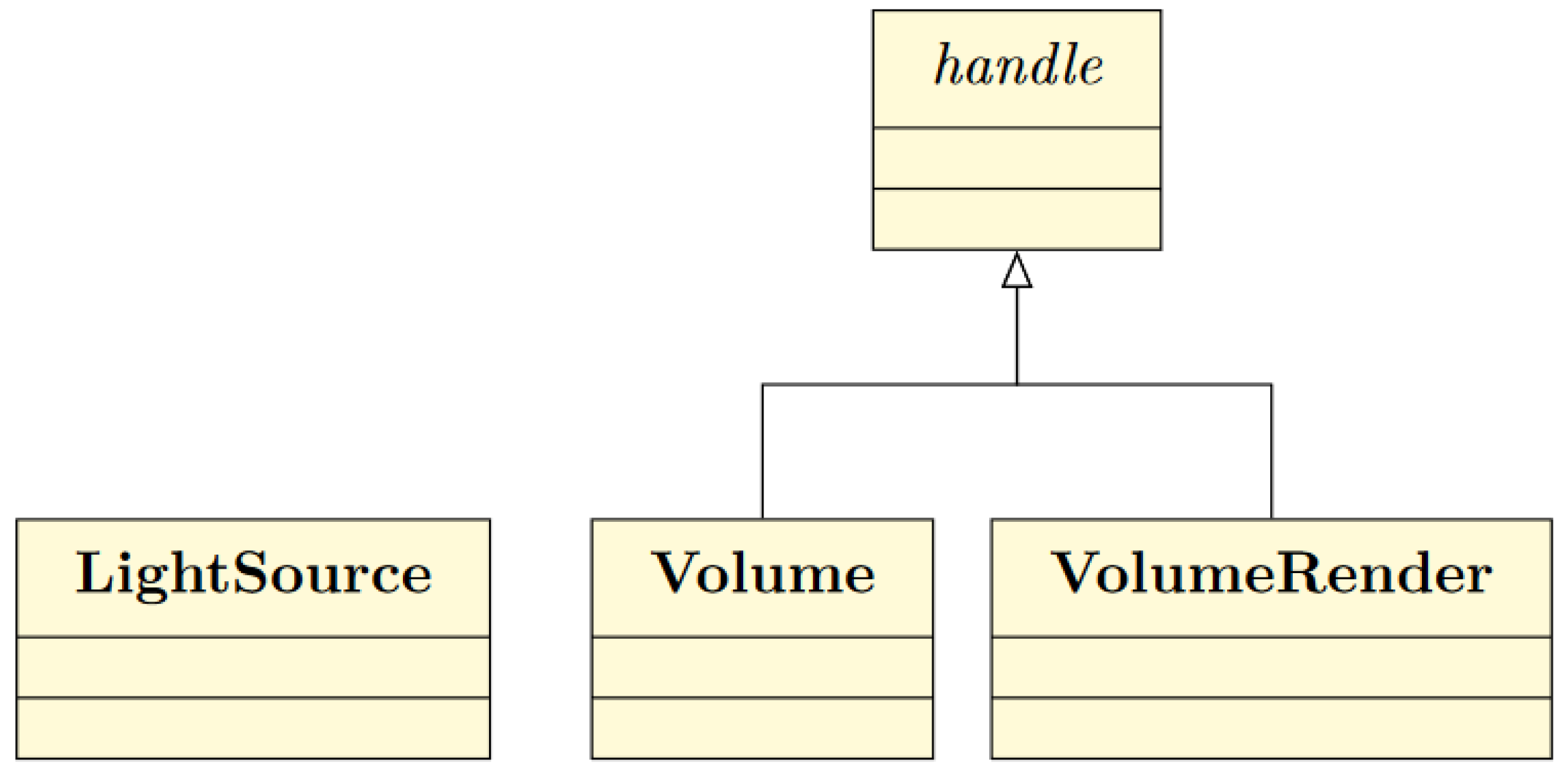
Figure 9.
To provide call by reference instead of call by value Volume and VolumeRender inherit handle. Additionally, the assignment of members does not return a deep copy of the object. Since, instances of LightSource consume low memory it does not inherit handle.
Figure 9.
To provide call by reference instead of call by value Volume and VolumeRender inherit handle. Additionally, the assignment of members does not return a deep copy of the object. Since, instances of LightSource consume low memory it does not inherit handle.
2.4.1. Handle Superclass
The realization of the memory management described in
Section 2.3.3 requires special techniques on the part of
MATLAB®. Usually a
MATLAB® class member work with call by value. But since we require the possibility to check the pointer of the volumes, call by reference is necessary. More precisely, on the C++ side we want to check whether the volumes are pointing to different pointer addresses or to the same one. Consequently only the unique volume data are copied to the GPU whereas the other assignments are realized by texture mapping to the assigned volume data. For us this seemed to be the most user-friendly way to implement our memory model.
Fortunately, MATLAB® offers the possibility for call by reference. A class that inherits from the special handle superclass automatically uses call by reference instead of call by value [29]. Hence, the class Volume inherits handle. Through this, all properties stored in a Volume object are pointers.
What is more, a regular value assignment through a setter can be expensive, since the old object is replaced by the new one. This new object is finally returned.
2.5. Case Study
2.5.1. Dataset
To demonstrate the capabilities of the renderer, we use a volumetric zebrafish larval image (ViBE-Z_72hpf_v1) created with ViBE-Z [
2]. Zebrafish embryos are widely used as a model organism in developmental biology and neurobiology due to their transparency and rapid development. High-resolution volumetric data of zebrafish larvals were acquired using 3D microscopy, providing detailed images of the internal structures essential for various research purposes. ViBE-Z uses multiple confocal microscope stacks and a fluorescent stain of cell nuclei for image registration and enhances data quality through fusion and attenuation correction. ViBE-Z can detect 14 predefined anatomical landmarks for aligning new data to the reference brain and can perform a colocalization analysis in expression databases for anatomical domains or subdomains. Specifically, the dataset used in this work contains zebrafish larval datasets. These include average silhouettes and brain structures with multiple channels. Each channel corresponds to different fluorescent markers that highlight various anatomical features.
2.5.2. Scene
In our rendering scenario, we created a movie depicting a 3D scene using two channels and a single light source. Volumetric data were sourced from an HDF5 file, specifically targeting datasets representing the average brain anatomy and the expression patterns of a specific structure. The resolution of the volume was [800, 500, 500].
The illumination setup was configured with a single light source, emitting white light. Parameters such as element size, focal length (set to 3.0), distance to the object (6), rotation angles, and an opacity threshold (0.95) were defined to put the object into scene. The image resolution was configured based on the dimensions of the volume data. The emission and absorption volume was set to the same data. The reflection volume was set to 1 for each voxel. The gradient was computed on the fly on the GPU.
In the rendering process, the zebrafish average brain image underwent a multi-step transformation. Initially, the entire volume was rendered with emission and absorption factors set to 1, resulting in a fully illuminated scene. Subsequently, a fading effect to the interior and half or the entire embryo was applied, gradually reducing its visibility, eventually ending up with the shell of one half of the average brain structure. This effect was achieved by adjusting the emission intensity of the volume data with the help of a pre-computed mask. The rendering of the brain structure did not experience any manipulations. After each rendering, the scene was rotated to provide a dynamic view from different angles. The rotation angles were calculated to achieve a rotation of 1200°over the course of the movie. The entire rendering consisted of three rendering loops:
rotation of the average brain by 150°(30 image frames)
fading out of the interior and one half while rotating 900°(180 image frames)
rotation of half of the average brain shell by 150°(30 image frames)
rendering of the brain structure with full rotation of 1200°(240 image frames)
Finally, the rendered frames from the average brain channel and the structure channel were combined to create a composite visualization of the zebrafish embryo. The resulting 240-image movie provides a complete visualization of the volumetric data, revealing structural details and expression patterns within the embryo.
The scene was rendered on a mobile workstation with NVIDIA A5000 with 16GB VRAM, Intel Core i9 11950H with 2.6GHz, 64GB RAM and SSD.
3. Results
3.1. Implementation
Our memory manager is designed to be user-friendly, offering MATLAB® classes that streamline the process of memory management. This allows users to easily allocate, deallocate, and manage memory within their MATLAB® projects without delving into complex CUDA programming. The source code is openly available on GitHub, making it accessible to the research and development community. This openness fosters innovation and allows for continuous improvement based on collective expertise and user feedback.
3.2. Volume Design
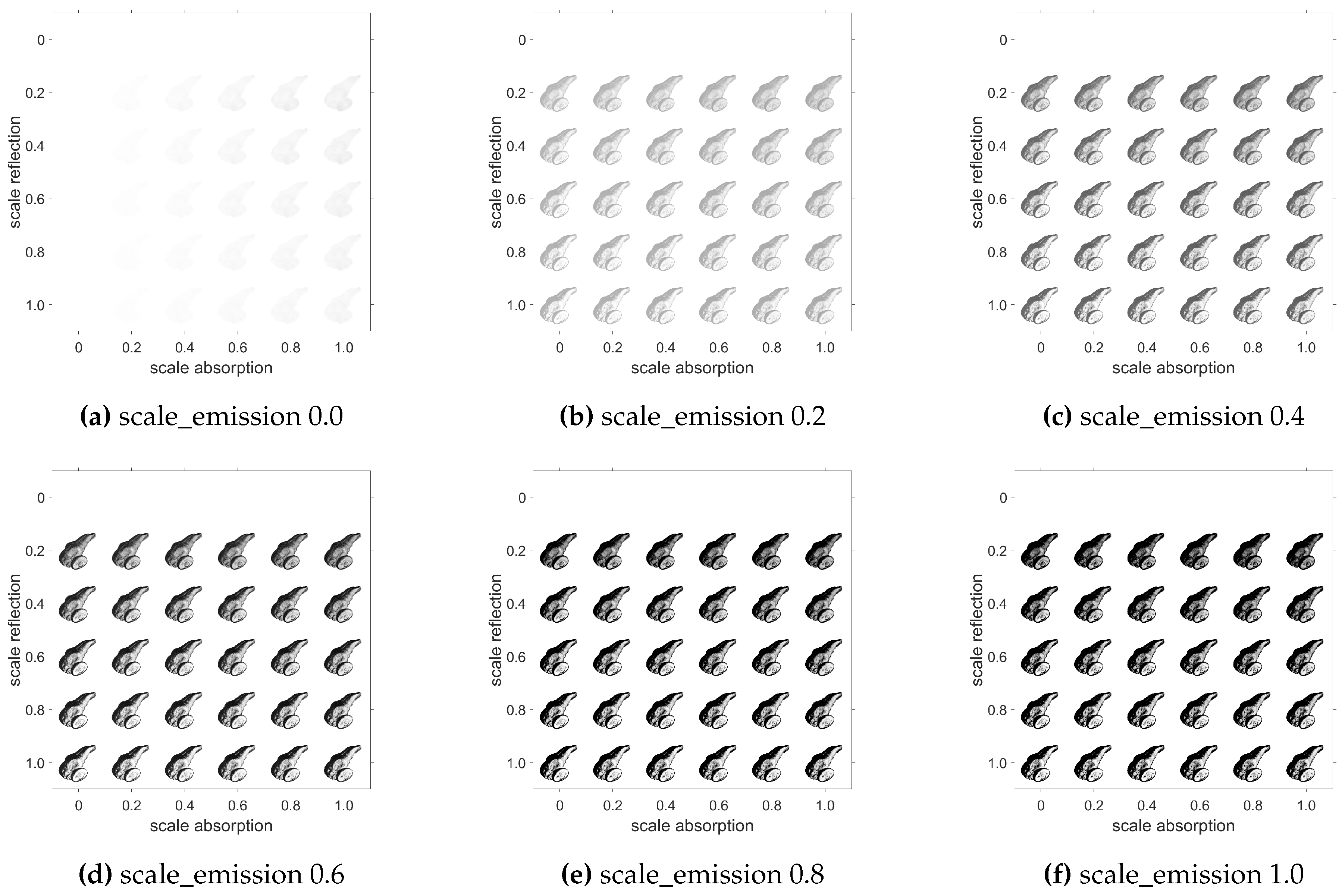
Our renderer supports the capability to define each volume, i.e. emission, absorption and reflection, allowing custom renderings to simulate different materials with different light properties. This is possible to do at a fine-granular scale for each voxel by defining distinct volumes or for an entire volume by a scalar. For our zebrafish volume, Figure 10 shows certain permutations of the scale value. The rendering setup is similar to the scene, but the absorption volume was set to a volume with value 1 for each voxel. The visual impact of the scales and therefore the different volumes becomes clearly discernible.
Figure 10.
Rendered images of a zebrafish embryo average brain with different emission, absorption and reflection factors.
Figure 10.
Rendered images of a zebrafish embryo average brain with different emission, absorption and reflection factors.
Obviously, without any emission, absorption and reflection information, the image is not visible. On the other hand, while increasing the absorption and adding some reflection, the opacity increases, as the light is reflected and absorbed by the object. High reflection values lead to a shiny appearance what can be counteracted by absorption, while no reflection at all makes the object disappear. Increasing the emission signals increases the effects. Although this illustration demonstrates the effect on the entire volume using the scaling values, it is important to emphasize that it is certainly possible to manipulate an object’s voxels to achieve specific effects in targeted areas. Boolean operations with masking can be used to select areas of interest.
3.3. Case Study
The rendered images demonstrate a high degree of realism, capturing the fine details of zebrafish embryo anatomy. By adjusting the emission, absorption, and reflection parameters, the visualizations effectively differentiate between various tissue types and fluorescent markers. The illumination setup further enhances the depth and contrast of the images, making the internal structures more discernible. Our case study consisted of 240 rendered image containing the zebrafish embryo average brain and some structure. The fish was rotated by 1200 °and one half of the average brain faded out in that image sequence. Figure 11 shows an excerpt of 8 images in which the object rotated 360°and the half of the average brain faded out. The entire video scene can be seen in the
Supplementary Materials. The GPU rendering took 119.32 seconds on our hardware setup.
Figure 11.
A rendered image of a zebrafish embryo average brain and some brain structures rendered in a separate pass, in pink color. In the sequence shown, the fish rotates 360°while one side of the average brain is faded out and finally rendered transparent, while the structure remains visible in pink. The first image is at the top left and the last at the bottom right.
Specifically, the first sequence took 4.57s, the second 58.58s and the third one 6.22s. The internal structure was rendered in 49.95s. Obviously, the second scene was the most expensive one, as due to the fading effect, parts of the volume were changed for each frame, requiring a data sync with the GPU. The computational runtime per frame in that sub-scene was 0.33s whereas the other scenes in average costed 0.20s, revealing the costs of host to GPU transfers.
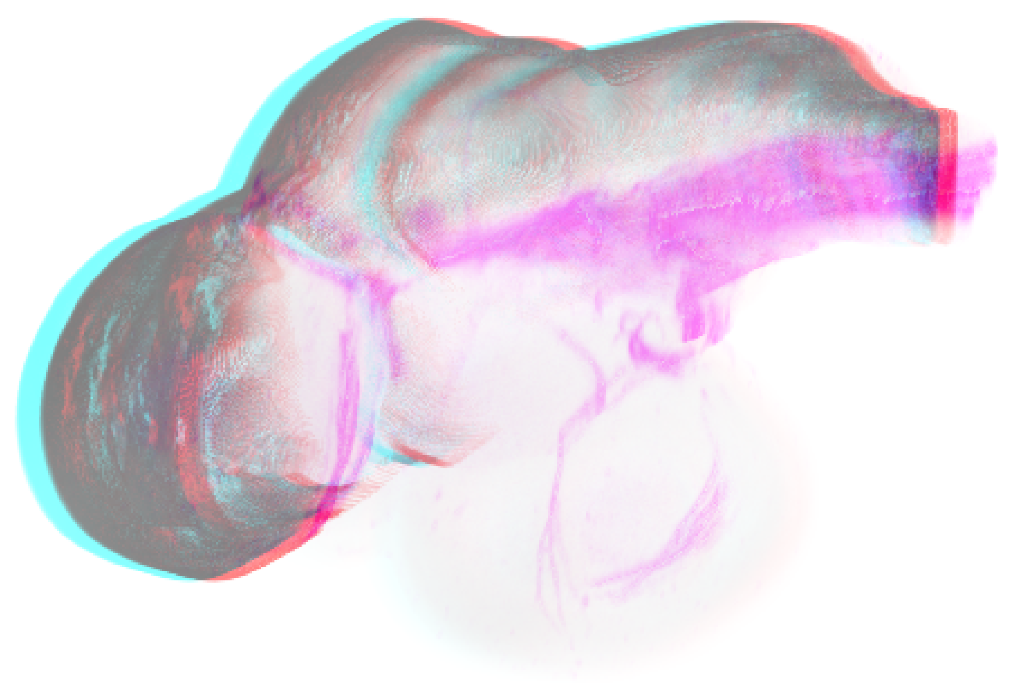
The ability to generate stereo images and animations adds another layer of depth to the visualizations, making it easier to comprehend the spatial relationships between different anatomical features. These realistic visualizations not only aid in detailed anatomical studies but also serve as valuable tools for educational purposes, providing clear and comprehensible images of complex biological structures. Figure 12 shows an image of the scene rendered in stereo using anaglyph. The entire scene in anaglyph can be seen in
Supplementary Materials.
Figure 12.
Rendered images of a zebrafish embryo average brain and some brain structure in anaglyph. Allures of the part which is fading out are still visible.
Figure 12.
Rendered images of a zebrafish embryo average brain and some brain structure in anaglyph. Allures of the part which is fading out are still visible.
4. Discussion
4.1. Principal Findings
With Volume Renderer we provide an offline renderer with a lot of functionalities. Due to the GPU-accelerated parallelization and the simplified render equation, the runtime can be kept low. Since the GPU memory size is very limited, the memory management we designed provides the opportunity to render volumes of larger resolutions.
Moreover, the render equation works with absorption and emission. Thus, it is possible to setup the rendering configuration to render multiple volumes in separated rendering passes in a way that the combination form a composite visualization.
Our illumination model interface enables the use of different illumination equations than proposed in this work. Several light sources with any light color intensities can be defined. This increases the realism of the scene and thus the spatial impression of the scene.
The MATLAB® interface is optimized for a simplified usage such that one can easily construct visualizations such as movie scenes and static images. Moreover, our renderer can render stereo images and combine them to an anaglyph or Side-By-Side stereo image. Since the values of the rendered images are stored in float types, the interface also provides normalization methods for both, single images and whole images sequences. Finally we optimized the runtime of the MATLAB® code. Therefore, and in order to be able to realize the memory management we make use of the handle class of MATLAB®, that allows us to use call by reference instead of call by value. In conclusion we provide a new convenient MATLAB® tool for volume rendering.
4.1.1. Boolean Operations
In the MATLAB® Volume Renderer, Boolean operations can be strategically utilized to manipulate emission, absorption, and reflection volumes, thereby enhancing the visualization of complex volumetric data. These operations — such as union, intersection, and difference — allow for intricate control over how different datasets are combined and visualized, providing deeper insights into the underlying structures.
Applying Boolean operations to emission volumes can help to isolate or highlight specific regions within a dataset. For instance, using the intersection operation, one can visualize only the overlapping areas of two emission datasets, which might represent regions where two different markers or conditions are present simultaneously. This can be particularly useful in medical imaging, where highlighting overlapping areas of different biomarkers can reveal critical pathological insights.
For absorption volumes, Boolean operations can be employed to enhance contrast and clarity. By subtracting one absorption volume from another, one can remove unwanted background data or emphasize specific features. For example, subtracting a general tissue absorption volume from a targeted region absorption volume can help in visualizing tumors or other anomalies with greater precision.
Reflection volumes benefit from Boolean operations by enabling the creation of more complex and realistic lighting models. Union operations can combine multiple reflection volumes to simulate the cumulative effect of different reflective surfaces within the dataset. This is particularly useful in visualizing complex structures where multiple reflective interfaces interact, such as in biomedical imaging of layered tissues or materials science.
Overall, the integration of Boolean operations in the MATLAB® Volume Renderer allows for more nuanced and precise control over emission, absorption, and reflection volumes, significantly enhancing the capability to visualize and interpret complex volumetric datasets. This enables researchers and clinicians to gain more detailed and actionable insights from their data.
4.2. Limitations
Modern deep learning approaches support features such as up-scaling [30], allowing for end-to-end training from image examples and eliminating the need for manual feature design, while supporting advanced visualization concepts like shading and semantic colorization [31] or even real-time rendering [32]. In contrast, our renderer lacks these advanced features out of the box but offers flexibility, enabling fully adjustable emission, absorption, and reflection parameters, along with customizable illumination setups. Also, our approach does not require extensive and potentially expensive training of models. However, one challenge might be the complexity of configuration options, which could overwhelm some users and might require to train them.
4.3. Future Works
To increase the realism and spatial impression of the rendered scenes the renderer could be enabled to use some shadowing techniques as described in [33]. Further, our renderer uses linear interpolation. To get more accurately interpolated values bi-cubic interpolation could be added as an additional option.
Furthermore, to increase usability and simplify the setup, the renderer could be extended with a user interface. An additional view showing the positioning of the light sources would also be beneficial. This could then also be extended for the development of video sequences in order to easily create camera paths and object motions by means of interpolation. However, these points are not planned to be implemented by us for the time being, but could be addressed by the community.
5. Conclusion
We demonstrate the effectiveness of our GPU-accelerated renderer in visualizing zebrafish embryo volumetric data with high realism. The flexibility in adjusting rendering parameters and the ability to create detailed, immersive visualizations make this tool an excellent choice for both research and educational applications. This integration with MATLAB provides a robust platform for biomedical researchers to analyze and visualize complex volumetric datasets within a familiar environment.
Supplementary Materials
The following supporting information can be downloaded at the website of this paper posted on
Preprints.org.
Author Contributions
Conceptualization, R.S; Data curation, R.S; Formal analysis, R.S; Investigation, R.S; Methodology, R.S; Project administration, R.S.; Resources, R.S; Software, R.S.; Supervision, R.S.; Validation, R.S; Visualization, R.S; Writing—original draft, R.S; Writing—review and editing, R.S. All authors have read and agreed to the published version of the manuscript.
Funding
This work was supported by the German Ministry for Education and Research grant number 01ZZ1804A, 01KX2121 and 01ZZ2304A.
Data Availability Statement
Acknowledgments
The Author would like to thank Olaf Ronneberger for his consultation. Many thanks also to Benjamin Ummenhofer, who provided support regarding the implementation with CUDA. Another big thank you goes to Johann Frei for his feedback on the manuscript.
Conflicts of Interest
The author declares no conflicts of interest.
References
- Kaufman, A.E. 43 - Volume Visualization in Medicine. In Handbook of Medical Imaging; Bankman, I.N., Ed.; Biomedical Engineering, Academic Press, 2000; pp. 713–730. [CrossRef]
- Ronneberger, O.; Liu, K.; Rath, M.; Rueß, D.; Mueller, T.; Skibbe, H.; Drayer, B.; Schmidt, T.; Filippi, A.; Nitschke, R.; et al. ViBE-Z: a framework for 3D virtual colocalization analysis in zebrafish larval brains. Nature Methods 2012, 9, 735–742. [Google Scholar] [CrossRef] [PubMed]
- Dickie, D.A.; Shenkin, S.D.; Anblagan, D.; Lee, J.; Blesa Cabez, M.; Rodriguez, D.; Boardman, J.P.; Waldman, A.; Job, D.E.; Wardlaw, J.M. Whole Brain Magnetic Resonance Image Atlases: A Systematic Review of Existing Atlases and Caveats for Use in Population Imaging. Frontiers in Neuroinformatics, 11.
- Kikinis, R.; Pieper, S.D.; Vosburgh, K.G. 3D Slicer: A Platform for Subject-Specific Image Analysis, Visualization, and Clinical Support. In Intraoperative Imaging and Image-Guided Therapy; Jolesz, F.A., Ed.; Springer, 2014; pp. 277–289. [CrossRef]
- Schindelin, J.; Arganda-Carreras, I.; Frise, E.; Kaynig, V.; Longair, M.; Pietzsch, T.; Preibisch, S.; Rueden, C.; Saalfeld, S.; Schmid, B.; et al. Fiji: an open-source platform for biological-image analysis. Nature Methods, 9, 676–682. Number: 7 Publisher: Nature Publishing Group. [CrossRef]
- Royer, L.A.; Weigert, M.; Günther, U.; Maghelli, N.; Jug, F.; Sbalzarini, I.F.; Myers, E.W. ClearVolume: open-source live 3D visualization for light-sheet microscopy. Nature Methods, 12, 480–481. Number: 6 Publisher: Nature Publishing Group. [CrossRef]
- Dhawan, A.P. Medical image analysis; John Wiley & Sons, 2011.
- Reyes-Aldasoro, C.C. Biomedical image analysis recipes in MATLAB: for life scientists and engineers; John Wiley & Sons, 2015.
- Mathotaarachchi, S.; Wang, S.; Shin, M.; Pascoal, T.A.; Benedet, A.L.; Kang, M.S.; Beaudry, T.; Fonov, V.S.; Gauthier, S.; Labbe, A.; et al. VoxelStats: A MATLAB Package for Multi-Modal Voxel-Wise Brain Image Analysis. Frontiers in Neuroinformatics, 10.
- Wait, E.; Winter, M.; Cohen, A.R. Hydra image processor: 5-D GPU image analysis library with MATLAB and python wrappers. Bioinformatics, 35, 5393–5395. [CrossRef]
- Explore 3-D Volumetric Data with Volume Viewer App - MATLAB & Simulink - MathWorks Deutschland.
- Kroon, D.J. Volume Render.
- Robertson, S. Ray Tracing Volume Renderer.
- Fujii, Y.; Azumi, T.; Nishio, N.; Kato, S.; Edahiro, M. Data Transfer Matters for GPU Computing. In Proceedings of the 2013 International Conference on Parallel and Distributed Systems, 2013, pp. 275–282. ISSN: 1521-9097. [CrossRef]
- Röttger, S.; Kraus, M.; Ertl, T. Hardware-Accelerated Volume and Isosurface Rendering Based on Cell-Projection, 2000.
- Wiki, O. Vertex Rendering — OpenGL Wiki,, 2022. [Online; accessed 23-May-2024].
- Lorensen, W.E.; Cline, H.E. Marching cubes: A high resolution 3D surface construction algorithm. SIGGRAPH Comput. Graph. 1987, 21, 163–169. [Google Scholar] [CrossRef]
- Levoy, M. Display of Surfaces from Volume Data. IEEE Computer Graphics and Applications 1988, 8, 29–37. [Google Scholar] [CrossRef]
- Max, N.L. Optical Models for Direct Volume Rendering. IEEE Trans. Vis. Comput. Graph. 1995, 1, 99–108. [Google Scholar] [CrossRef]
- Wikipedia. Volume ray casting — Wikipedia, The Free Encyclopedia. 2023. Available online: http://en.wikipedia.org/w/index.php?title=Volume%20ray%20casting&oldid=1146671341 (accessed on 18 April 2023).
- Shannon, C.E. Communication in the presence of noise. In Proceedings of the Proceedings of the Institute of Radio Engineers (IRE), 1949, Vol. 37, pp. 10–21.
- Henyey, L.; Greenstein, J. Diffuse radiation in the galaxy. The Astrophysical Journal 1941, 93, 70–83. [Google Scholar] [CrossRef]
- Blinn, J.F. Models of light reflection for computer synthesized pictures. SIGGRAPH Comput. Graph. 1977, 11, 192–198. [Google Scholar] [CrossRef]
- Porter, T.; Duff, T. Compositing digital images. ACM SIGGRAPH Computer Graphics 1984, 18, 253–259. [Google Scholar] [CrossRef]
- Ikits, M.; Kniss, J.; Lefohn, A.; Hansen, C. GPU GEMS Chapter 39, Volume Rendering Techniques, 5th ed.; Addison Wesley, 2007; chapter 39.4.3 Rendering.
- Bourke, P. Calculating Stereo Pairs, 1999.
- Williams, A.; Barrus, S.; Morley, R.K.; Shirley, P. An Efficient and Robust Ray-Box Intersection Algorithm. journal of graphics, gpu, and game tools 2005, 10, 49–54. [Google Scholar] [CrossRef]
- NVIDIA Corporation. NVIDIA CUDA C Programming Guide, 2011. Version 4.0.
- The MathWorks, I. Object-Oriented Programming. Object-Oriented Programming 2011, R2011b. [Google Scholar]
- Devkota, S.; Pattanaik, S. Deep Learning based Super-Resolution for Medical Volume Visualization with Direct Volume Rendering, 2022, [arXiv:cs.GR/2210.08080].
- Weiss, J.; Navab, N. Deep Direct Volume Rendering: Learning Visual Feature Mappings From Exemplary Images, 2021, [arXiv:cs.GR/2106.05429].
- Hu, J.; Yu, C.; Liu, H.; Yan, L.; Wu, Y.; Jin, X. Deep Real-time Volumetric Rendering Using Multi-feature Fusion. In Proceedings of the ACM SIGGRAPH 2023 Conference Proceedings, New York, NY, USA, July 2023; SIGGRAPH ’23, pp. 1–10. [CrossRef]
- Ikits, M.; Kniss, J.; Lefohn, A.; Hansen, C. GPU GEMS Chapter 39, Volume Rendering Techniques, 5th ed.; Addison Wesley, 2007; chapter 39.5.1 Volumetric Lighting.
|
Disclaimer/Publisher’s Note: The statements, opinions and data contained in all publications are solely those of the individual author(s) and contributor(s) and not of MDPI and/or the editor(s). MDPI and/or the editor(s) disclaim responsibility for any injury to people or property resulting from any ideas, methods, instructions or products referred to in the content. |
© 2024 by the author. Licensee MDPI, Basel, Switzerland. This article is an open access article distributed under the terms and conditions of the Creative Commons Attribution (CC BY) license (https://creativecommons.org/licenses/by/4.0/).
