Computational Test for Conditional Independence (with Categorical Variables)

Conditional Independence (CI) testing is fundamental in statistical analysis. For example, CI testing helps validate causal graphs or longitudinal data analysis with repeated measures in causal inference. CI testing is difficult, especially when testing involves categorical variables conditioned on a mixture of continuous and categorical variables. Current parametric and non-parametric testing methods designed for continuous variables and can quickly fall short in the categorical case. This paper presents a computational approach for CI testing for categorical data types, which we call computational conditional independence (CCI) testing. The test procedure is based on permutation and combines machine learning prediction algorithms and Monte Carlo Cross-Validation. We evaluated the approach through simulation studies and assessed the performance against alternative methods; the generalized covariance measure (GCM) test, the kernel conditional independence (KCI) test, and testing with multinomial regression. We find that the computational approach to testing has utility over the alternative methods, and we can achieve better control over type-I-error rates. We hope this work can expand the toolkit for CI testing for practitioners and researchers.

Keywords:

Subject: Computer Science and Mathematics - Probability and Statistics

1. Introduction

Robust conditional independence (CI) testing in statistics is arduous and, in some sense, impossible. Despite this, CI testing is a central task in applied statistical research. For instance, in causal inference [1], a causal graph, which can form the basis of a causal estimator, can be validated through testing a set of implied marginal independence and CI statements [1,2]. Because of its importance, considerable work [3,4,5,6,7,8,9] has been allocated to create tests for CI, especially for continuous cases. However, no statistical test or algorithm is universally superior for detecting CI between variables of all types in all situations, as stated by the no-free-lunch theorem for CI testing in [3]. Different methods may perform better or worse depending on the specifics of the underlying data-generating structure. Therefore, one should develop and explore several testing methods for CI testing for various data characteristics and types, using both asymptotic and computational approaches. Because of the flexibility of regression and classification algorithms in machine learning, state-of-the-art prediction modeling is an excellent starting point for testing CI [3]. With this in mind, this article proposes and explores a computational method based on machine learning classification for testing CI. Although the approach can, in principle, work with various data types, we will focus our attention on CI testing involving the special cases when there is a mixture of categorical and continuous variables in the CI statement. To our knowledge, no suitable testing method exists in such cases.

Conditional independence testing

A common notation of CI between random variables Y and X given Z is

Y ⊥ ⊥ X | Z \Leftrightarrow X ⊥ ⊥ Y | Z,

(1)

where Z can be extended to a set of variables

Z

. One can also express CI using probability distributions;

p (Y ∣ X, Z) = p (Y ∣ Z)

where

p (Z) > 0

, or

p (X, Y ∣ Z) = p (X ∣ Z) p (Y ∣ Z)

, which is to say that given that we know

Z = z

neither X nor Y carries information about each other’s distribution [10].

When Y and X are continuous and the conditioning set

Z

has a mixture of variable types, numerous testing methods for CI exist. The two state-of-the-art and readily available methods are the kernel-based test (KCI test) from [4], and the generalized covariance measure (GCM test) [3]. The KCI test is based on the foundational idea that the uncorrelatedness between functions in kernel Hilbert spaces can characterize statistical independence and CI. The test uses kernel matrices associated with the variables to construct a test statistic based on these matrices. As it stands, the test is designed for continuous data. However, since the KCI-test uses a kernel function, it can potentially be modified to account for other data types by changing the function. The GCM test is based on the fact that the standardized covariance between residuals from the two generic regressions

y = h (z)

and

x = g (z)

follow, under the null hypothesis and given relatively mild assumptions, an asymptotic standard normal distribution. Although the GCM test statistic is designed for continuous data types, in our experience, it handles binary data well.

When dealing with purely categorical variables within the CI statement, i.e., categorical variables with more than two categories, the literature on testing methods is somewhat scarcer. In cases where Y, X, and Z in Equation 1 are all categorical or of discrete types, the conditional

χ^{2}

test, also known as the Cochran-Mantel-Haenszel test, is a well-known and reliable test. The

χ^{2}

test requires sufficiently many observations in each conditioned category to function optimally [11]. Testing based on mutual information is also a common choice for testing CI with only discrete data [12]. However, in CI statements where either X or Y or both are categorical and Z consist of continuous variables, or a mix of continuous variables and other types, there are, to our knowledge, no reliable testing methods available. For example, [2] suggests employing multinomial regression or abstaining from testing altogether. Testing CI with a parametric model is problematic as it relies on specifying the correct, or close to correct, functional form.

To create a CI testing framework for categorical variables, we suggest using machine learning classification algorithms in combination with permutation and Monte Carlo cross-validation (MCCV) to create a null distribution. To obtain the test statistic and p-value, one utilizes the same machine learning classification model without permutation with one train test split. As an extension to this, one can also create a test-statistic distribution with MCCV and assess a distribution of p-values, which is a helpful extension in cases where testing is done with a limited sample size. The organization of our article is as follows: Section 2 details our proposed testing procedure, Section 3 presents the simulation study exploring key aspects such as type I error rates and power under difficult testing conditions. In Section 4, we present an illustrative example of the testing procedure, and test results of multiple simulations over a range of multivariate distributions. A general discussion follows in Section 5, and concluding remarks in Section 6.

2. Computational Testing with Categorical Variables

Our proposed computational procedure for testing CI, we call computational conditional independence test (CCI test). As mentioned above, the method is, in principle, quite flexible. Still, we focus on the case where the aim is to test CI between two categorical variables.

Let Y and X represent categorical variables with

j = 1 \dots J

and

k = 1 \dots K

categories respectively. Under the null hypothesis of CI, a classification model for Y,

P (Y = k ∣ X, Z)

, should perform equivalently to a model using a permuted

X^{*}

instead of X. Hence, we posit the null and alternative hypotheses as follows:

\begin{matrix} H_{0} : & M (P (Y = k ∣ X^{*}, Z)) = M (P (Y = k ∣ X, Z)) \\ \Leftrightarrow M (P (X = j ∣ Y^{*}, Z)) = M (P (X = j ∣ Y, Z)), \end{matrix}

(2)

\begin{matrix} H_{1} : & M (P (Y = k ∣ X^{*}, Z)) \neq M (P (Y = k ∣ X, Z)) \\ \Leftrightarrow M (P r (X = j ∣ Y^{*}, Z)) \neq M (P r (X = j ∣ Y, Z)), \end{matrix}

(3)

where M denotes a suitable performance metric for the classification model, estimating the probability

P ()

, such as Kappa scores or log loss.

2.1. Establishing a Null Distribution by MCCV

A fundamental challenge in statistical testing lies in controlling the significance level, defined as the false positive rate or type I error rate. We manage this error rate by estimating an empirical null distribution of metric scores using Monte Carlo Cross-Validation (MCCV) in combination with permutation. Generally, statistical testing based on permutation is a robust alternative when fundamental assumptions by parametric and nonparametric tests are violated [13]. MCCV is a resampling technique typically used to assess machine learning models’ performance by randomly partitioning data into training and testing sets. For each iteration, MCCV randomly selects a subset of data used for training, and the remaining observations serve as the test (validation) set.

The first step in setting up a test is to choose between a classification model for Y or for X. Tree-based models robust against overfitting when predicting new data are probably the best choice, however we will discuss this further in Section 2.3. For now, let us assume that we have a robust classification model for Y and therefore

M (P (Y = k ∣ X^{*}, Z)) = M (P (Y = k ∣ X, Z))

is the null hypothesis.

Now we can estimate the empirical null distribution(s): For each MCCV iteration; we first permute X into

X^{*}

, then randomly split the data into a training set, of size

p N

, and testing set, of size

(1 - p) N

, and then train a classification model for Y using

X^{*}

and the condition set

Z

using the training set data. We then calculate the classification performance metric using the testing set. After many iterations, this approach theoretically derives the empirical distribution of metric scores under the null being true.

2.2. Calculating p-Values

Once the null distribution is established, we generate a test statistic from a single estimation of the classification model for Y using the original, unpermuted X. Again, we split the data into a random training and testing set, estimate the classification model using the training data, and calculate the performance metric using the testing data. Under the null hypothesis, the metric score calculated using an unpermuted X, should be a random draw from the empirical null distribution.

Conversely, if the alternative hypothesis is true, including the unpermuted X should enhance classification performance, thereby facilitating the p-value calculation based on the test statistic’s relative position within the null distribution. The (one-sided test) p-value (e.g., using log loss as the performance metric) is given by,

p = \frac{\sum (Null \leq test statistic) + 1}{n + 1},

(4)

where

\sum (Null \leq test statistic)

represents the count of instances in the null distribution that are less than or equal to the test statistic, and n is the total number of observations in the null distribution. Note that the direction of ≤ in Equation 4 depends on which metric score is used. If, for instance, we use Kappa scores, where a higher value means a better performing model, we would have to change ≤ to ≥. The ”+1” in the numerator and the denominator is a correction factor that prevents a p-value of 0 and makes the p-value somewhat more conservative. A p-value of 0 is good to avoid since it implies absolute certainty.

Testing CI by classification modeling for an accurate p-value calculation demands a large sample. When the sample size is small, the statistical power is often low. With an insufficient sample size, minor yet meaningful improvements in performance by including the original X rather than the permuted

X^{*}

may not be detected from a single train-test split of the unpermuted data. Therefore, when testing CI with a relatively small sample, one should not rely on one p-value but instead do multiple test train splits and examine the resulting distribution of p-values, providing additional robustness to the analysis. Basic statistical theory says that given a true null hypothesis, the p-values should be distributed approximately uniform(0,1). By calculating and plotting several p-values in Quantile-Quantile (QQ) plots, one can visually assess if the empirical p-values approximately follow the distribution against their theoretical counterparts. It is important to emphasize that evaluating the distribution of p-values is not a test per see, and one cannot and should not test statistically if the empirical distribution of p-values follows a theoretical uniform distribution, for instance, by a Kolmogorov-Smirnov test [14]. Firstly, such tests assume an underlying continuous distribution, which is not the case. Secondly, these tests are susceptible to sample size, where a large sample size almost guarantees a low p-value, and the ”sample size” can be manipulated by the number of MCCV iterations. Thirdly, the Kolmogorov-Smirnov and other similar tests test against uniformity, which is, in this case, wrong.

2.3. Choice of Classification Model and Performance Metric

The computational method described above assumes that modeling the classification probabilities

P (Y = k | X, Z)

P (X = j | Y, Z)

allows us to extract all relevant information from the conditioned variables. Significantly, the method relies on the robustness of the classification model in generalizing from the training data to the testing data. Although an optimal classification model cannot be guaranteed, modern off-the-shelf tree-based machine learning algorithms such as XGBoost (eXtreme Gradient Boosting) [15] have demonstrated remarkable performance in predicting class categories and robustness against overfitting training data. Other alternatives are random forest [16] or other gradient boosting framework such as lighGBM [17] or CatBoost [18].

The choice of performance metric or metrics carries implications, as different metrics evaluate various aspects of a classification model’s performance. The metrics we use in this article are log loss and Kappa scores; they were chosen because they are well-known, continuous, and have somewhat different qualities. Kappa scores are better when comparing the same model across different datasets, especially when categories are unbalanced. Log loss offers greater precision than Kappa scores by accounting for the certainty of class predictions, which is relevant. We have yet to determine which metrics best suit the task; we will attempt to shed some light on this question in Section 3.

3. Simulation Setup

The simulation study aims to evaluate the performance of CCI testing and compare it against some ”established” methods. We also aim to assess and compare the two performance metrics log loss and Kappa scores.

The basic simulation set-up is that we draw data from seven different multivariate distributions with four variables

{Z_{1}, Z_{2}, X, Y}

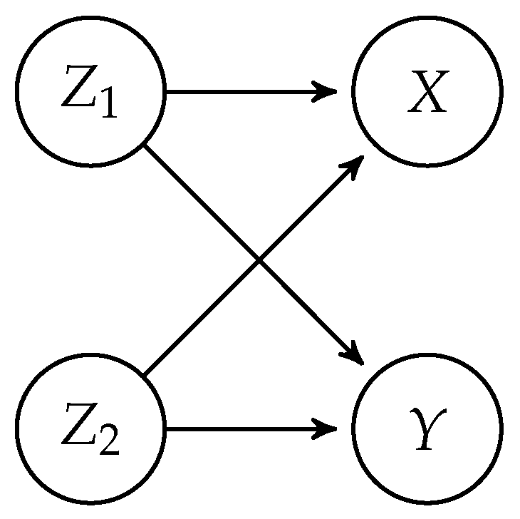
. The dependencies between the variables are as shown in the directed acyclic graph depicted in Figure 1, which implies the CI statement

Y ⊥ ⊥ X | Z_{1}, Z_{2} \Leftrightarrow X ⊥ ⊥ Y | Z_{1}, Z_{2}

. All multivariate distributions, involve non-linear relations between

Z_{1}

and

Z_{2}

, made such that testing CI is not trivial. In all simulations,

Z_{1}

and

Z_{2}

are continuous variables, either normally or uniformly distributed, while both X and Y are categorical. A short non-technical description of the data-generating functions follows, and pseudo codes of the functions are found in Appendix B.

Interaction: interactions between Z1 and Z2.

Z_{1}

and

Z_{2}

are standard normal, and X and Y are set deterministically by a series of if statements which assign values from 0 to 3, depending on the quadrant in which the coordinate (

Z_{1}

Z_{2}

) falls into, creating an interaction between

Z_{1}

and

Z_{2}

ExpLog: Exponential and logarithmic distributions.

Z_{1}

and

Z_{2}

are standard normal. X is influenced by the exponentiation of the sum of

Z_{1}

and

Z_{2}

where the categories of X change as the sum exceeds certain thresholds. The categorization of Y is based on the logarithm of the absolute value of

Z_{1}

plus one, added to

Z_{2}

passing specific thresholds. The simulation imitates the modeling of exponential and logarithmic growth.

PolyData:

Z_{1}

and

Z_{2}

are standard normal. The categorization of X is based on different polynomial combinations of

Z_{1}

and

Z_{2}

. The categorization of Y similarly involves higher-degree polynomials of

Z_{1}

and

Z_{2}

TrigData:

Z_{1}

is uniform(

- π

π

), while

Z_{2}

is standard normal. X is created based on adding sin(

Z_{1}

) and cos(

Z_{2}

), and the categorization of Y is based on subtracting sin(

Z_{1}

) and cos(

Z_{2}

). The simulation imitates the modeling of cyclic phenomena.

Non-Linear: A non-linear and trigonometric simulation testing if CI testing methods are robust against complex real-world data patterns involving periods or cycles such as in time-series analysis.

ComplexCategorization: A simulation that emulates data scenarios where multiple factors and their interactions influence outcomes.

Multinomial This simulation is based on multinominal regression equations, with non-linear effects from

Z_{1}

and

Z_{2}

. This simulation aims to generate a data set where the influence of

Z_{1}

is relatively weak and, therefore, harder to test

Y ⊥ ⊥ X | Z_{2}

In all testing scenarios, we employ the XGBoost classification model from the R package xgboost [19], using default parameter settings with two exceptions: the learning rate is set to

e t a = 0.1

, and the number of boosting trees is set at

n t r e e s = 120

. The train test split ratio in MCCV is set to 0.825, meaning for each iteration, a random portion of 82.5% of the data is utilized as training data. Additionally, we use the createDataPartition-function from the caret-package [20] to balance the class distributions within the splits. As ”feature” variables in the XGBoost classification model we include

Z_{1}

and

Z_{2}

and their transformations: squared and cubed.

We also conduct CI testing with the GCM test, the KCI test and multinominal regression. The GCM test, conducted via the R package GeneralizedCovarianceMeasure [21], uses default settings. The KCI test, implemented through the R package CondIndTests [22], has its Gaussian Process hyperparameter routine disabled to reduce computation time, note that the KCI test demands extensive computational resources with increasing sample sizes. Multinomial regression analyses are performed using the nnet package [23], incorporating

Z_{1}

Z_{2}

, and their squared and cubed terms as predictors.

We ran our simulations over three sample sizes (500, 800, and 2000) and simulated 100 datasets from the multivariate distributions for each size. For each dataset, we tested

Y ⊥ X ∣ Z_{1}, Z_{2}

for assessing the type I error rate. We test

Y ⊥ X ∣ Z_{2}

to assess power, and note that type II error is equal to 1 - power. For all tests, we set the significant level at 5 %, which means that if we test a true null hypothesis, about 5 % of tests should be refuted.

4. Results

4.1. Illustrative Example

Before we present the simulation result, we will illustrate the testing procedure using a specific simulated example. Our dataset comprises 800 simulated observations drawn from the interaction multivariate distribution. We hypothesize that the null hypothesis –

M (P r (Y = k ∣ X^{*}, Z_{1}, Z_{2})) = M (P r (Y = k ∣ X, Z_{1}, Z_{2}))

– will not be rejected by the test.

For each MCCV iteration, we start by permuting X into

X^{*}

, and then train the classification model

\hat{P} (y | x^{*}, z_{1}, z_{2})

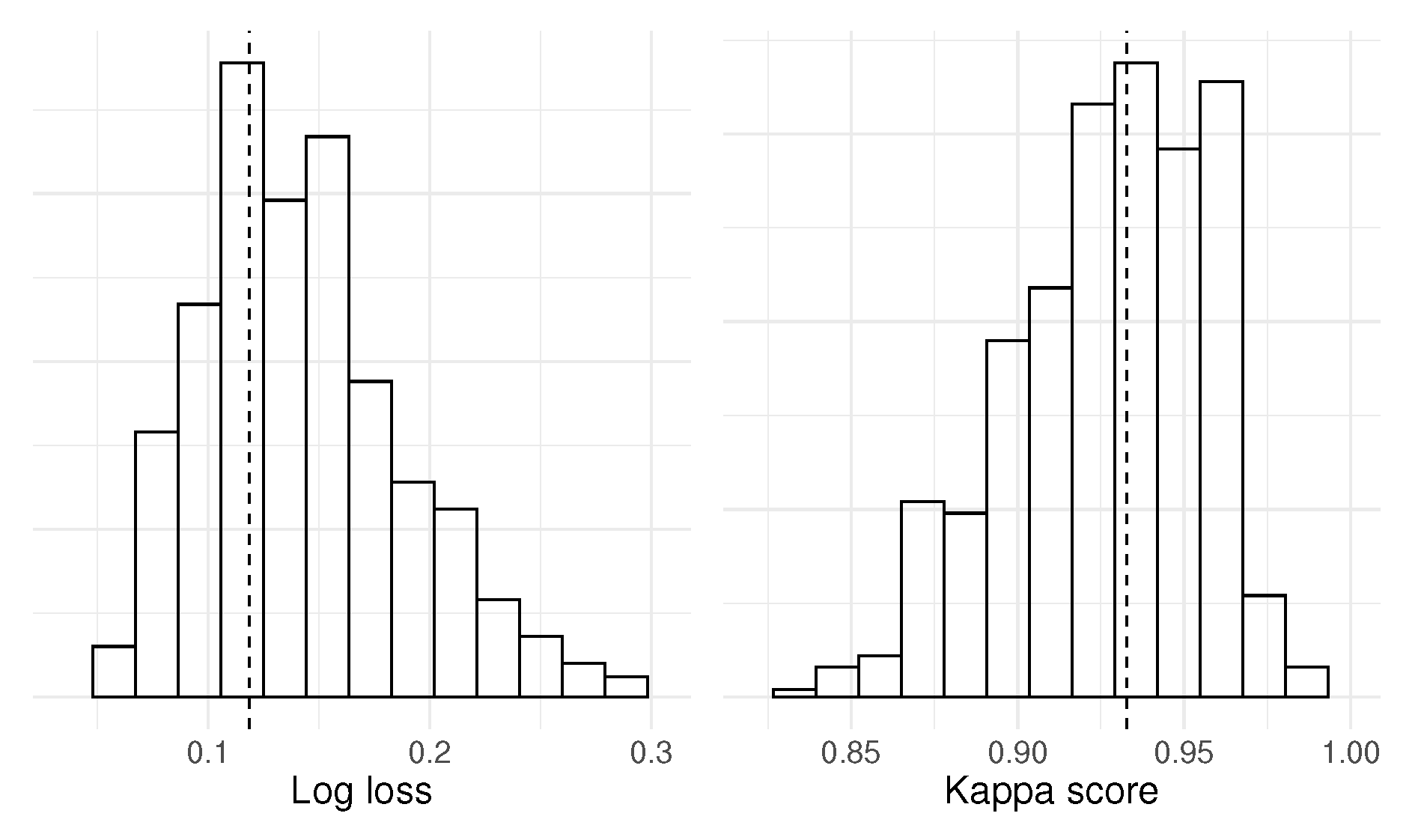
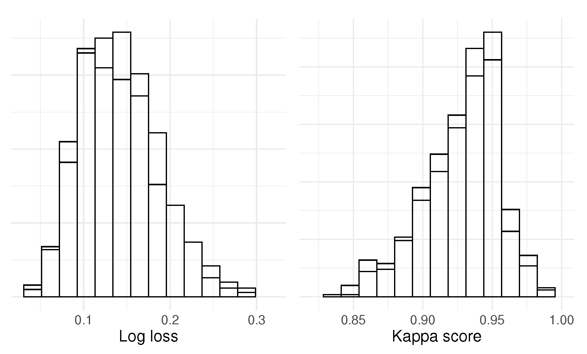
using 82.5 % of the data, and the performance metrics log loss and Kappa score were calculated on the remaining data. We performed 1000 iterations to create the null distributions of log loss and Kappa scores shown in Figure 2. Now, swap the permuted

X^{*}

with the unpermuted X. Perform one instance of a train-test split to estimate

\hat{p} (y | x, z_{1}, z_{2})

, and again, the log loss and Kappa score are extracted by predicting using the testing data. The resulting one-sided p-values are 0.34 (log loss) and 0.36 (Kappa score), and the null hypothesis is not rejected.

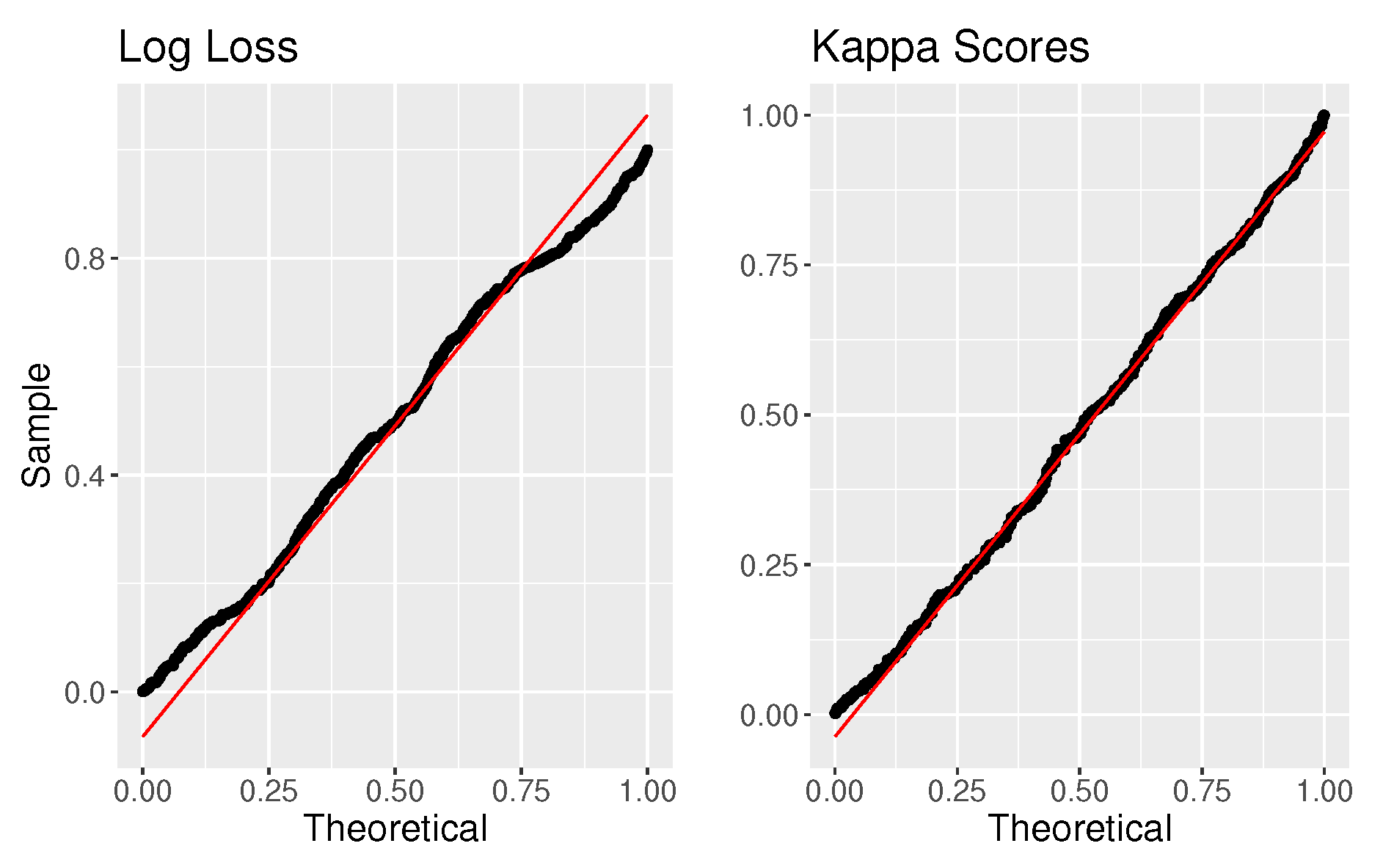
To show that we have control over type I error in this case, we can estimate the corresponding test statistic distributions and overlay the null distributions, which is shown in Figure 3. The distributions almost perfectly overlay each other, and if we then calculate a p-value for every test statistic, we get that the distribution of p-values follows a uniform(0,1) distribution, as shown in Figure 4. Since the p-values are uniformly distributed, we control the type I error rate under a true null, and 5 % of the p-values are less than 0.05.

Further, to illustrate how the test works in the opposite case, we remove

Z_{1}

from the test, which gives the null hypothesis

M (P r (Y ∣ X^{*}, Z_{2})) = M (P r (Y ∣ X, Z_{2}))

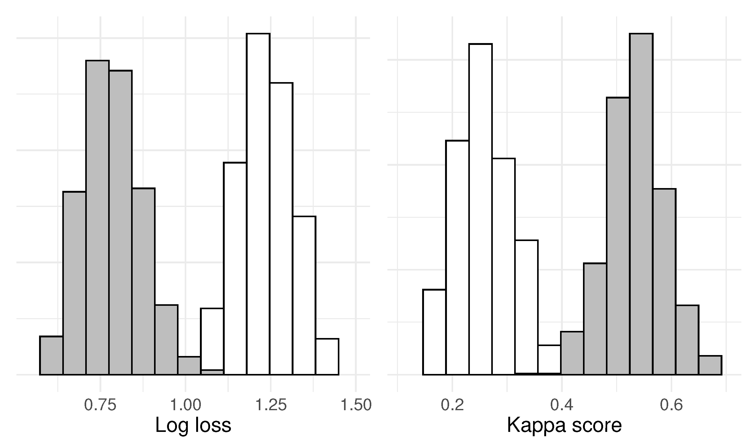
– which we hypothesize will be rejected by the test. The new null distributions and test statistic distributions are given in Figure 5 – the two distributions have almost zero overlap. A random test statistic yields p-values of 0.000099 for both log loss and Kappa score1.

4.2. Testing with one p-Value

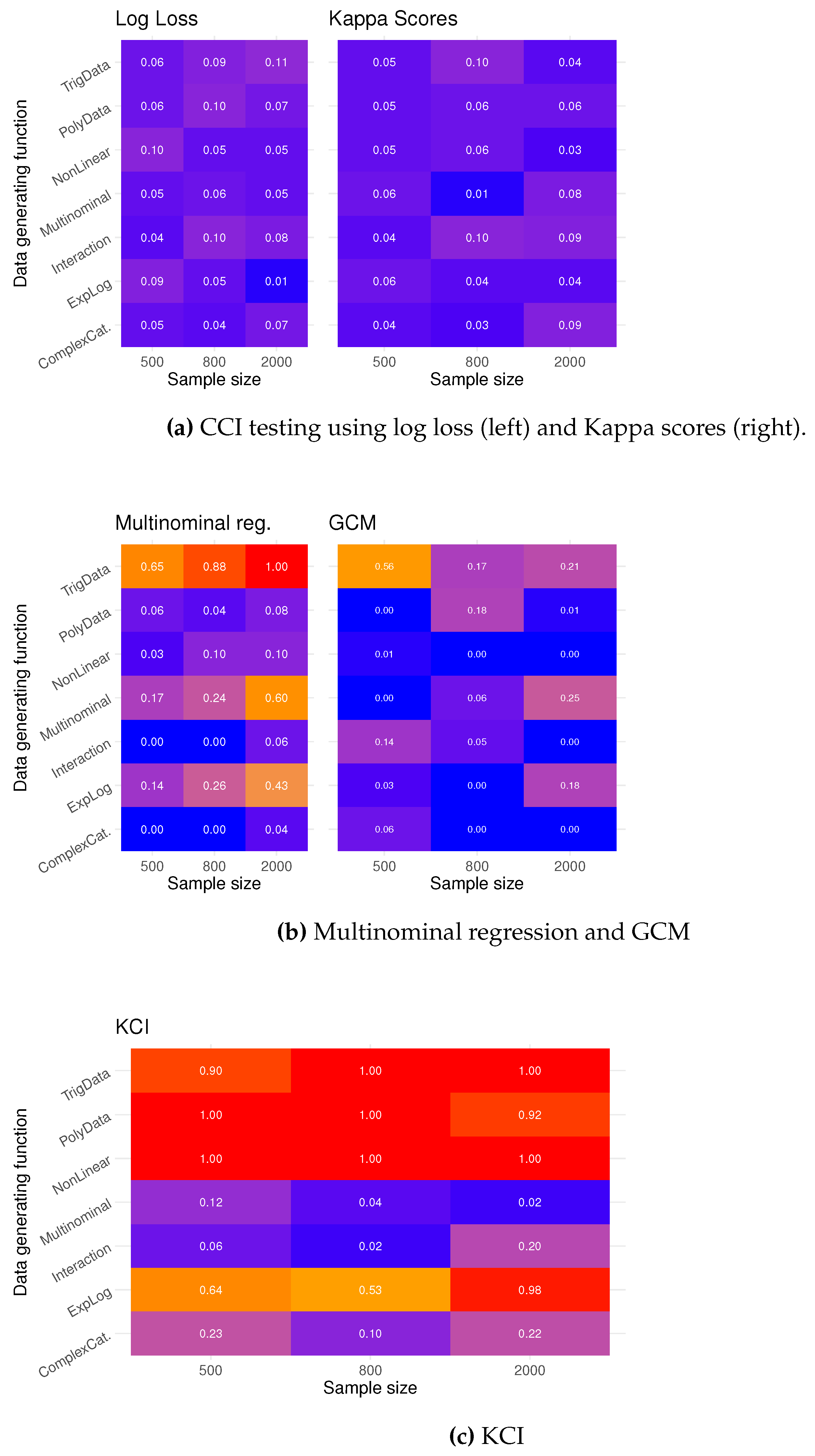
In the heat and overlay plots in Figure 6, we see the type I error rate for 100 tests for each sample size using the seven proposed simulations. The computational testing procedure exhibits fairly good type I error across different data-generating functions, especially if one were to compare against alternative methods, shown in the heat plots in Figure 6 and Figure 6. Data simulated from the TrigData seems like the simulation scenario where it is most difficult to control the error rate.

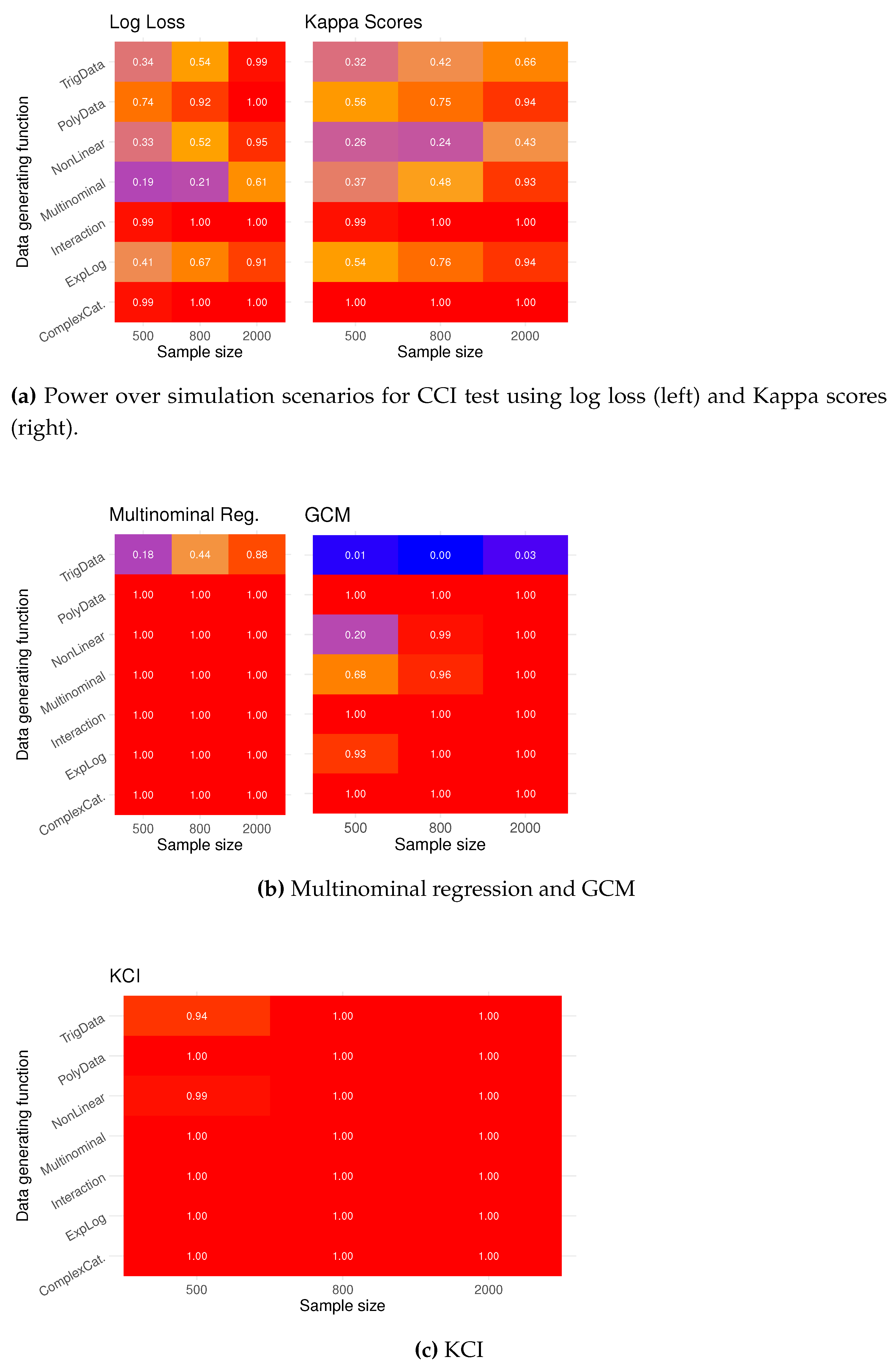
In Figure 7, we see the estimated power of the computational testing procedure. The power is calculated as the proportion of p-values less than 0.05 when testing

Y ⊥ ⊥ X | Z_{2}

. The power increases with the sample size, and using log loss seems to give more power than Kappa scores. The possibility for low power with small samples emphasizes that computational testing is a ”large” sample method due to its reliance on machine learning classification methodology.

The other methods, multinominal regression, GCM test (Figure 7), and KCI test (Figure 7), have high power, but testing CI with categorical variables with these methods can be very misleading as the type I error rate can be as high as 100 %.

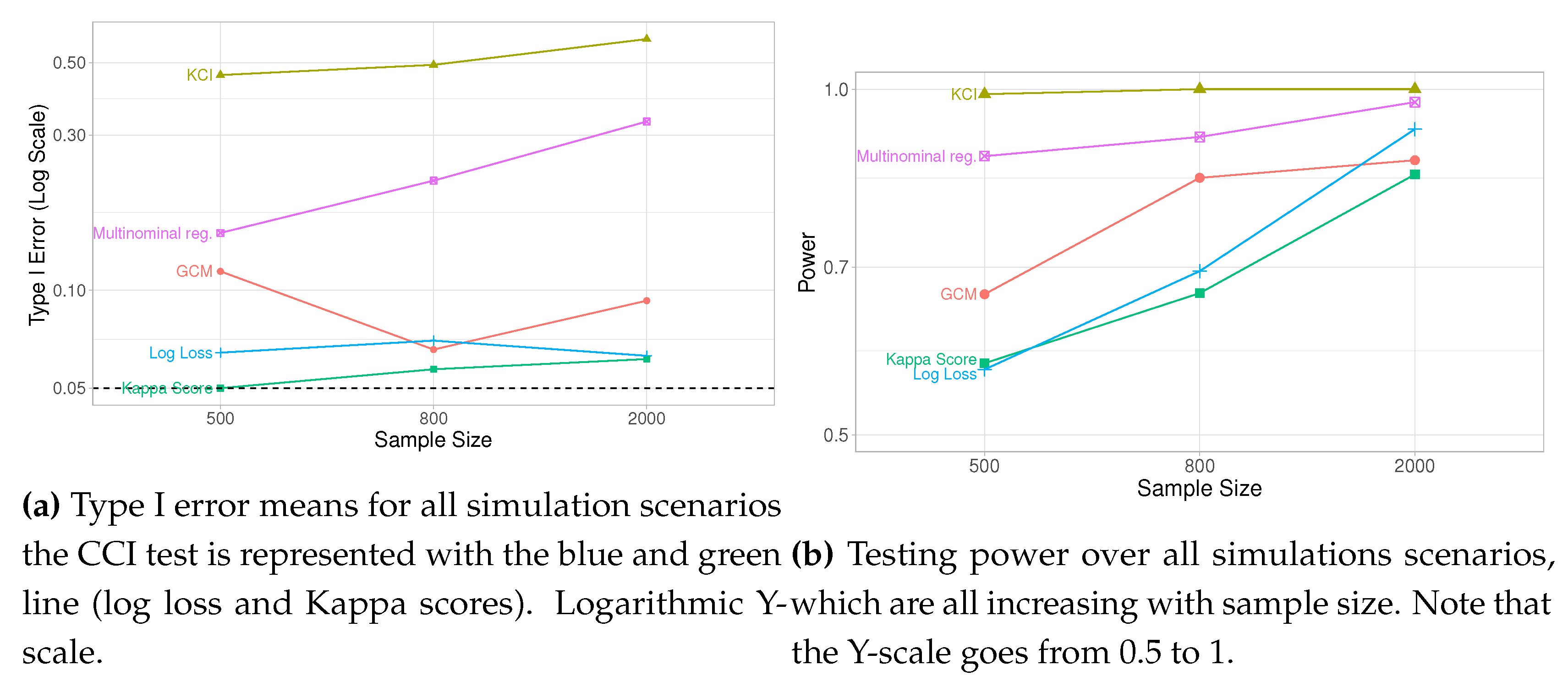
In Figure 8a and Figure 8b, we have averaged the type I error and power over all simulations, which leads us to conclude that the proposed computational testing is a viable alternative to existing methods.

4.3. Assessing with p-Value Distribution

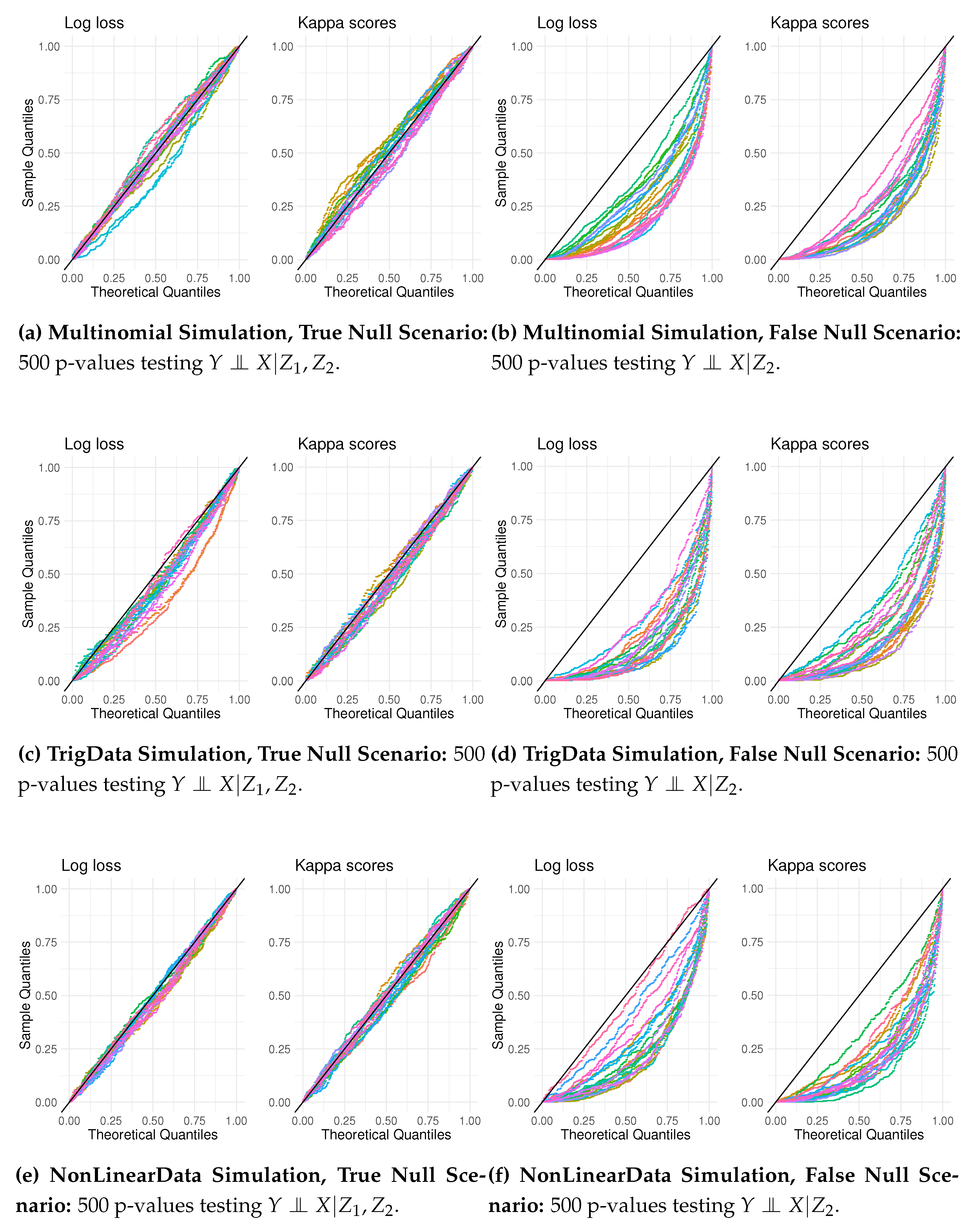
To assess how CCI can analyze CI statements by calculating a distribution of p-values instead of relying on one p-value, we generated data from the three simulation scenarios, Multinomial, TrigData, and NonLinearData, where a false CI is the most challenging to test. For each simulation scenario, we generated 20 datasets, each containing 500 observations. For testing both the true null of

M (P (Y = k ∣ X^{*}, Z_{1}, Z_{2})) = M (P (Y = k ∣ X, Z_{1}, Z_{2}))

, and an erroneous null;

M (P (Y = k ∣ X^{*}, Z_{2})) = M (P (Y = k ∣ X, Z_{2}))

. For each data set (i.e., 60 data sets), we estimated 500 p-values by estimating an empirical null distribution and the corresponding distribution of test statistics.

In Figure 9, the 500 p-value points for each test are color-coded. Each QQ plot has 20 lines of color-code dots, one for each data set. When testing a true null, we get the plots in Figure 9, Figure 9 and Figure 9. There is a close alignment with the theoretical uniform distribution, which suggests good adherence to the null hypothesis. Some degree of variability, as in minor deviations from the diagonal, is acceptable. Kappa scores seem to have somewhat less idiosyncratic variation.

The QQ plots, depicted in Figure 9, Figure 9 and Figure 9, show the distribution of p-values for testing

Y ⊥ X | Z_{2}

. The points, especially using Kappa scores as the underlying metric, have a notable deviation compared to their theoretical counterparts. This deviation suggests a systematic tendency towards lower p-values than those expected under the null hypothesis, indicating a likely violation of the null, the desired outcome. One can note that when assessing the QQ plots, one should evaluate the difference between the points and the line based on vertical distance [24].

Kappa scores provide better testing performance using QQ plots. With Kappa scores, p-values seem more stable around the diagonal line when testing a true null and more deviate from it when testing a false null.

In addition to providing a testing framework in small samples, using QQ plots has some other benefits. QQ plots can reveal patterns that can indicate fundamental errors, for instance, if the p-values tend to be high, meaning that the points would bend upwards to the left; such a pattern can indicate the non-independence of samples or highly correlated features.

5. Discussion

When testing CI with categorical variables we can expect that CCI outperforms the continuous testing methods GCM and KCI since, in these cases, the fundamental assumptions of GCM and KCI are violated. Although the basic assumptions of multinominal regression are not violated when used to test CI, any parametric method is restrictive as the functional form needs to be defined. As the simulation results show, the better performance of CCI is not due to superiority in rejecting false hypotheses but both better control of type I error and increasing power as sample size increases.

Given

Y ⊥ ⊥ X | Z

, it should not matter if Y or X is the dependent variable in the classification algorithm in CCI. A criterion for choosing Y or X is if some variable in Z is highly correlated with either Y or X. Then, choose the one with the highest correlation as the dependent variable to reduce the correlation among the features in the classification model. In practical settings, we recommend running a single case to see if there are any estimation problems by choosing Y or X as the dependent variable. Furthermore, to ensure optimal results, we recommend tuning the hyperparameters of the classification model using a separate dataset not involved in the final testing. This practice can potentially improve the performance and reliability of the test results. Given that CCI testing relies on machine learning techniques, familiarity with these methodologies is recommended for practitioners employing the CCI test.

5.1. Assumptions and Limitations

There are two key implicit assumptions in the CCI testing procedure. Firstly, the XGBoost classification modeling must be able to unravel potentially complex relationships between the variables. Secondly, the XGBoost classification algorithm must generalize well to unseen data. Of course, there is no way to ensure this, but a few steps can increase the likelihood of good performance. Include transformation of the original features; we include squared and cubed terms in our example, but a richer set is possible. A second strategy is to pre-tune the classification model; if there is sufficient data, setting aside a portion of the data dedicated to tuning the classification model before testing might increase the models’ ability to use all the information when testing for CI.

The computational method is inherently more computationally intensive than most other CI testing methods, except KCI testing with a large sample size. For instance, with 2,000 observations from the Interaction simulation, creating a null distribution with 1,000 iterations on a standard laptop with 8 GB RAM and a 1.60 GHz processor using a single core required approximately 13 minutes. For larger datasets, especially those exceeding 10,000 observations, employing methods such as subsampling may help mitigate computational demands. Furthermore, optimizing computation time will also depend on settings in the XGBoost classification model; hence, adopting specific strategies informed by expert knowledge is recommended for efficiency improvements in practical applications.

No matter how many simulation examples are applied, computational methods can only be shown to work for the specific datasets and scenarios provided. We have attempted to provide a range of difficult testing scenarios to show that computational testing is viable in cases where one needs to establish CI between categorical variables, even when the underlying data structure is complex. However, computational methods are usually less efficient and less generalizable compared to asymptotic methods.

5.2. Strengths

In computational statistics, permutation is a well-known tool for breaking any observed association between variables and forms the basis of many tests. Testing CI by permutation is an intuitive and versatile concept that, in principle, can be applied to any CI testing situation involving various data types. CCI is flexible and demands few assumptions about the nature of the data, only that the observations are independent. As shown through simulations, CCI can handle complex relationships between variables and is, in principle, scalable as you can expand the condition set

Z

”indefinitely”, making it applicable to many settings.

Using an off-the-self classification method offers transparency into any specific test. Practitioners can further analyze test results by studying the classification model itself; for example, looking at feature contributions can give insights into the nature of any CI statement. In combination, using QQ plots can give practitioners deeper insights into the behavior of the data under the null hypothesis.

5.3. Further Research

There are several possibilities for further exploration in computational testing of CI, and testing CI in general. For instance, although our simulation examples are highly non-linear, they are also low dimensional; the number of observations is much larger than the number of variables. Exploring computational CI in high-dimensional settings, where the number of variables may approach or exceed the number of observations, is perhaps a natural next step. Another avenue of research is to replace the performance metrics log loss and Kappa scores and instead use conditional mutual information criteria or Shapley values to create the null distribution.

Another avenue for further explorations is a more robust assessment of QQ plots, for instance, by a lineup test introduced by [25]. The lineup test concept consists of embedding a plot that contains the actual data effect among several plots of randomized data or noise and seeing if people can identify the plot with actual data.

6. Conclusion

This paper has demonstrated a practical application of CI testing, employing a computational approach that leverages permutation, the XGBoost classification algorithm, and MCCV. The proposed method fills a gap in the empirical validation of CI with categorical variables, enhancing CI testing for practitioners in real-world scenarios.

While advantageous for testing CI with categorical data, CCI has limitations. First and foremost, it requires a relatively large sample to achieve sufficient power, it demands a somewhat working knowledge of classification modeling, and it is computationally demanding, especially with a large feature set.

Author Contributions

Conceptualization, Christian B. H. Thorjussen, Ingrid Måge, Kristian H. Liland and Lars Erik Solberg; methodology, Christian B. H. Thorjussen, Ingrid Måge, Kristian H. Liland and Lars Erik Solberg; software, Christian B. H. Thorjussen and Kristian H. Liland; validation, Christian B. H. Thorjussen; formal analysis, Christian B. H. Thorjussen; data curation, Ingrid Måge and Christian B. H. Thorjussen; writing—original draft preparation, Christian B. H. Thorjussen; writing—review and editing, Christian B. H. Thorjussen, Ingrid Måge, Kristian H. Liland and Lars Erik Solberg; visualization, Christian B. H. Thorjussen; supervision, Ingrid Måge, Kristian H. Liland and Lars Erik Solberg; project administration, Ingrid Måge, Kristian H. Liland; funding acquisition, Ingrid Måge. All authors have read and agreed to the published version of the manuscript.

Funding

This research was funded by "Stiftelsen for Landbrukets Næringsmiddelforskning" (SLNF), The Research Council of Norway through the projects SFI Digital Food Quality (project number 309259), and by the Norwegian Agricultural Food Research Foundation through the project Precision Food Production (project number 314111)

Data Availability Statement

R scripts used in this manuscript is available at the Github repository https://github.com/ChristianBHT/CI_article.

Conflicts of Interest

The authors declare no conflict of interest. The funders had no role in the design of the study; in the collection, analyses, or interpretation of data; in the writing of the manuscript; or in the decision to publish the results.

Abbreviations

The following abbreviations are used in this manuscript:

CI	Conditional Independence
GCM test	Generalized Covariance Measure test
KCI test	Kernel Conditional Independence test
CCI test	Computational Conditional Independence test
MCCV	Monte Carlo Cross-Validation
QQ	Quantile-Quantile
XGBoost	Extreme Gradient Boost

Appendix A. Testing with Continous Data

Although we focus on testing with categorical variables in the article, CCI can also be used with various data types. In this appendix section, we assess the performance of the CCI test by comparison to the GCM test, when Y, X,

Z_{1}

, and

Z_{2}

are all continuous variables. Again we use the dependency structure depicted in Figure 1 and generate data from five multivariate distributions. Below are descriptions of various multivariate functions that generate simulated data sets:

Normal Data Function: Generates a dataset where both $Z_{1}$ and $Z_{2}$ are drawn from standard normal distributions. The variables X and Y are also normally distributed, influenced by the sum of $Z_{1}$ and $Z_{2}$ , showcasing a simple additive model.
Non-Linear Normal Data Function: Creates data with $Z_{1}$ and $Z_{2}$ as normal variables, while X includes a nonlinear transformation involving the exponential of the product $Z_{1} \times Z_{2}$ , with normal noise added. Y is formed by the product $Z_{1} \times Z_{2}$ with additional normal noise.
Uniform Noise Data Function: This function produces a dataset where $Z_{1}$ and $Z_{2}$ are normally distributed, but X and Y are derived from a linear combination of $Z_{1}$ and $Z_{2}$ plus a term involving their product, with uniform noise added to introduce non-normal error distribution and test model robustness against such noise.
Exponential Noise Data: Similar to the uniform noise mode, it replaces the uniform noise with exponential noise with a rate parameter $a = 1$ . This function is useful for examining the impact of skewed, heavy-tailed noise on statistical inferences.
Poisson Noise Function: Generates data where $Z_{1}$ and $Z_{2}$ are normally distributed, but X and Y include Poisson-distributed noise influenced by the product of $Z_{1}$ and $Z_{2}$ .
Sinusoidal Data: This function creates data where $Z_{1}$ and $Z_{2}$ are normal, but X and Y involve sinusoidal transformations modulated by an exponential decay function based on the sum of $Z_{1}$ and $Z_{2}$ . The sinusoidal component depends on linear combinations of $Z_{1}$ and $Z_{2}$ .

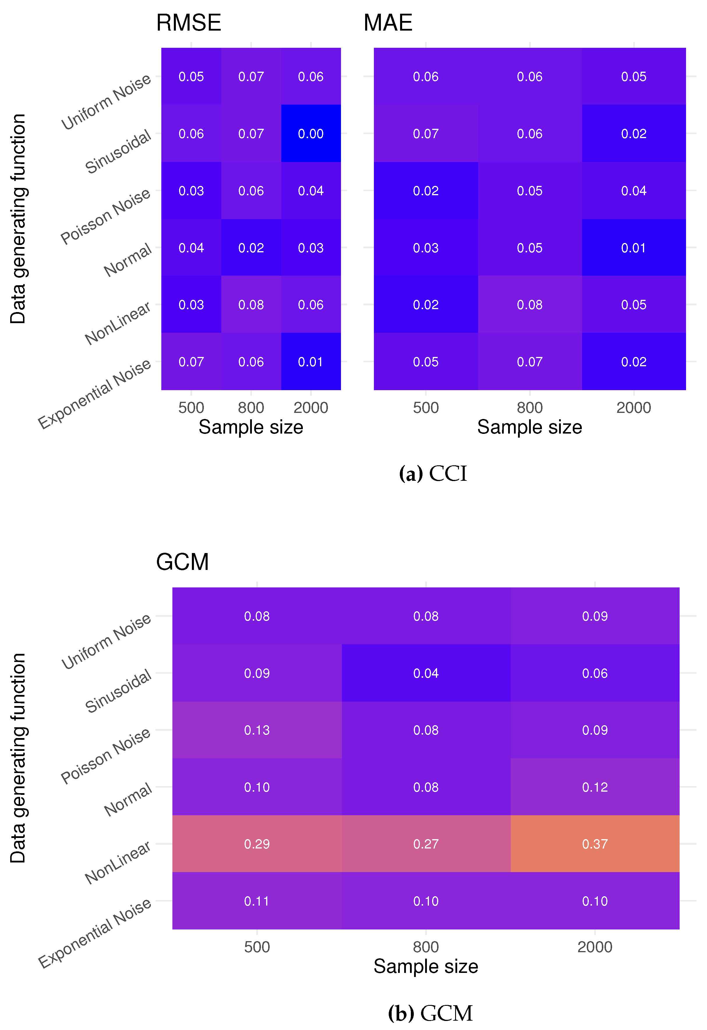
For each simulated distribution and test method, we perform 100 tests under both a true null and a false null hypothesis. We calculate the type I error rate by looking at the number of significant results at a significant level

α = 0.05

. The power of the test under each simulated multivariate distribution is estimated by the number of rejected tests under a false null. The performance metrics for computation testing are Root Mean Square Error and Mean Absolute Error (MAE).

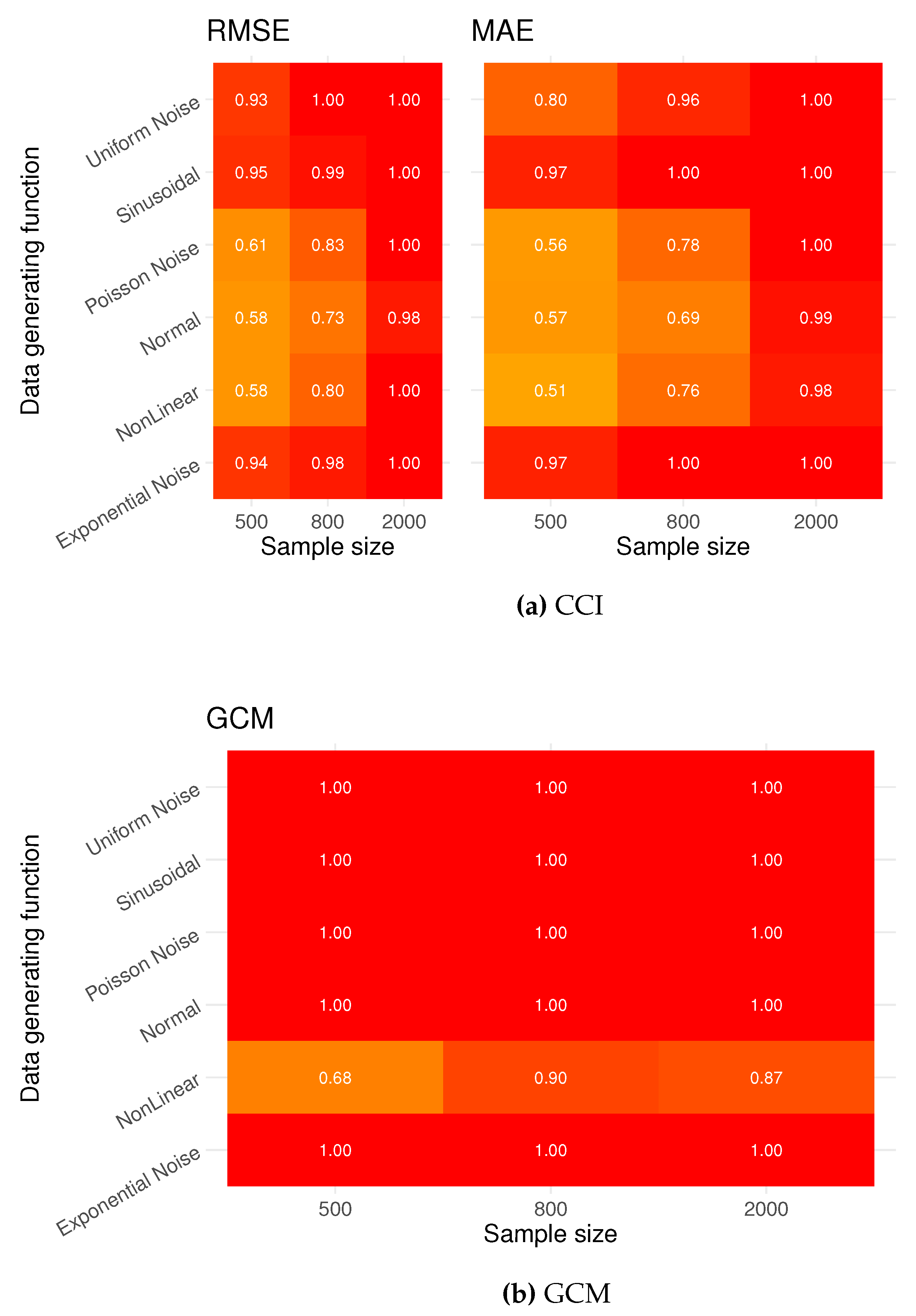
In Figure A1, we see type I error rates; for these simulations examples, CCI testing is more conservative than GCM (Figure A1). The GCM test exhibits a relatively high type I error in scenarios involving the Non-Linear, Normal, and Exponential Noise distributions. This high error rate is likely due to GCM’s reliance on the even distribution of residuals around the regression line, making it susceptible to outliers, which can be produced by these generating functions. Assessing the power of the CCI testing, we see that with a sample of 2000, CCI testing can consistently reject a false null; GCM has a superior rejection rate with lower sample sizes.

Figure A1. Type I error rates: Rejection rates testing a true null

Y ⊥ ⊥ X | Z_{1}, Z_{2}

. The CCI test is considerably more conservative than GCM, and CCI performs better in these scenarios, as GCM relies on the assumption of ”well behaved” residuals.

Figure A1. Type I error rates: Rejection rates testing a true null

Y ⊥ ⊥ X | Z_{1}, Z_{2}

. The CCI test is considerably more conservative than GCM, and CCI performs better in these scenarios, as GCM relies on the assumption of ”well behaved” residuals.

Figure A2. Power: Rejection rates testing the false null

Y ⊥ ⊥ X | Z_{2}

. The results of the CCI test are given in Figure A1 using the performance metrics RMSE and MAE. At sample size 500 CCI testing has low power. The GCM shows high power in almost all scenarios.

Figure A2. Power: Rejection rates testing the false null

Y ⊥ ⊥ X | Z_{2}

. The results of the CCI test are given in Figure A1 using the performance metrics RMSE and MAE. At sample size 500 CCI testing has low power. The GCM shows high power in almost all scenarios.

In conclusion, we see that CCI testing is a viable testing method in continuous cases and can compete with the GCM test, given a sufficient sample size.

Appendix B. Pseudocode for Multivariate Distributions Generating Functions for Categorical Data

The R functions created to generate data are presented in pseudo-code to convey the procedural steps in generating datasets.

Algorithm 1 Interaction Data (Interaction)

1:: $Z_{1} \leftarrow$ Draw N samples from $N (0, 1)$
2:: $Z_{2} \leftarrow$ Draw N samples from $N (0, 1)$
3:: for $i \leftarrow 1 to N$ do
4:: if $Z_{1} [i] < 0 and Z_{2} [i] < 0$ then
5:: $X [i] \leftarrow 0$
6:: else if $Z_{1} [i] < 0 and Z_{2} [i] \geq 0$ then
7:: $X [i] \leftarrow 1$
8:: else if $Z_{1} [i] > = 0 and Z_{2} [i] < 0$ then
9:: $X [i] \leftarrow 2$
10:: else
11:: $X [i] \leftarrow 3$
12:: end if
13:
14:: if $Z_{1} [i] < 0 + Z_{2} [i] < - 1$ then
15:: $Y [i] \leftarrow 0$
16:: else if $Z_{1} [i] < 0 + Z_{2} [i] < 0$ then
17:: $Y [i] \leftarrow 1$
18:: else if $Z_{1} [i] < 0 + Z_{2} [i] < 1$ then
19:: $Y [i] \leftarrow 2$
20:: else
21:: $Y [i] \leftarrow 3$
22:: end if
23:: end for
24:: return ${Z_{1}, Z_{2}, X, Y}$

Algorithm 2 Exponent and Logarithmic Data (ExpLog)

1:: $Z_{1} \leftarrow$ Draw N samples from $N (0, 1)$
2:: $Z_{2} \leftarrow$ Draw N samples from $N (0, 1)$
3:: for $i \leftarrow 1$ to n do
4:: Compute $t e m p X \leftarrow exp (Z 1 [i]) + Z 2 [i]$
5:: if $t e m p X > 1$ then
6:: $X [i] \leftarrow 3$
7:: else if $t e m p X > 0$ then
8:: $X [i] \leftarrow 2$
9:: else if $t e m p X > - 1$ then
10:: $X [i] \leftarrow 1$
11:: else
12:: $X [i] \leftarrow 0$
13:: end if
14:: Compute $t e m p Y \leftarrow log (| Z 1 [i] | + 1) + Z 2 [i]$
15:: if $t e m p Y > 0.5$ then
16:: $Y [i] \leftarrow 3$
17:: else if $t e m p Y > 0$ then
18:: $Y [i] \leftarrow 2$
19:: else if $t e m p Y > - 0.5$ then
20:: $Y [i] \leftarrow 1$
21:: else
22:: $Y [i] \leftarrow 0$
23:: end if
24:: end for
25:: return ${Z_{1}, Z_{2}, X, Y}$

Algorithm 3 Polynomial Data (PolyData)

1:: Initialize number of samples N
2:: $Z_{1} \leftarrow$ Draw N samples from $N (0, 1)$
3:: $Z_{2} \leftarrow$ Draw N samples from $N (0, 1)$
4:: for $i \leftarrow 1$ to N do
5:: if $Z_{1} {[i]}^{2} + Z_{2} {[i]}^{2} > 2$ then
6:: $X [i] \leftarrow 3$
7:: else if $Z_{1} {[i]}^{2} + Z_{2} [i] > 0.5$ then
8:: $X [i] \leftarrow 2$
9:: else if $Z_{1} [i] + Z_{2} {[i]}^{2} > 0$ then
10:: $X [i] \leftarrow 1$
11:: else
12:: $X [i] \leftarrow 0$
13:: end if
14:: if $Z_{1} {[i]}^{3} + Z_{2} [i] > 1$ then
15:: $Y [i] \leftarrow 3$
16:: else if $Z_{1} {[i]}^{2} + Z_{2} {[i]}^{2} > 0$ then
17:: $Y [i] \leftarrow 2$
18:: else if $Z_{1} [i] + Z_{2} {[i]}^{3} > - 1$ then
19:: $Y [i] \leftarrow 1$
20:: else
21:: $Y [i] \leftarrow 0$
22:: end if
23:: end for
24:: return ${Z_{1}, Z_{2}, X, Y}$

Algorithm 4 Trigonometric Data (TrigData)

1:: Initialize number of samples N
2:: $Z_{1} \leftarrow$ Draw N samples from $N (0, 1)$
3:: $Z_{2} \leftarrow$ Draw N samples from $N (0, 1)$
4:: for $i \leftarrow 1$ to n do
5:: if $s i n (Z_{1} [i]) + c o s (Z_{2} [i]) > 1$ then
6:: $X [i] \leftarrow 3$
7:: else if $s i n (Z_{1} [i]) + c o s (Z_{2} [i]) > 0$ then
8:: $X [i] \leftarrow 2$
9:: else if $s i n (Z_{1} [i]) > - 1$ then
10:: $X [i] \leftarrow 1$
11:: else
12:: $X [i] \leftarrow 0$
13:: end if
14:: if $c o s (Z_{1} [i]) - s i n (Z_{2} [i]) > 1$ then
15:: $Y [i] \leftarrow 3$
16:: else if cos( $Z_{1} [i]) - s i n (Z_{2} [i]) > 0$ then
17:: $Y [i] \leftarrow 2$
18:: else if $c o s (Z_{1} [i]) > - 1$ then
19:: $Y [i] \leftarrow 1$
20:: else
21:: $Y [i] \leftarrow 0$
22:: end if
23:: end for
24:: return ${Z_{1}, Z_{2}, X, Y}$

Algorithm 5 Non-linear Data (Non-Linear)

1:: Initialize number of samples N
2:: $Z_{1} \leftarrow runif (N, - 1, 1)$
3:: $Z_{2} \leftarrow runif (N, - 1, 1)$
4:: for $i \leftarrow 1$ to N do
5:: if $sin (Z_{1} [i] \times π) + Z_{2} [i] > 1$ then
6:: $X [i] \leftarrow 3$
7:: else if $sin (Z_{1} [i] \times π) + Z_{2} [i] > 0.5$ then
8:: $X [i] \leftarrow 2$
9:: else if $sin (Z_{1} [i] \times π) + Z_{2} [i] > 0$ then
10:: $X [i] \leftarrow 1$
11:: else
12:: $X [i] \leftarrow 0$
13:: end if
14:: if $cos (Z_{1} [i] \times π) + Z_{2} [i] > 1$ then
15:: $Y [i] \leftarrow 3$
16:: else if $cos (Z_{1} [i] \times π) + Z_{2} [i] > 0.5$ then
17:: $Y [i] \leftarrow 2$
18:: else if $cos (Z_{1} [i] \times π) + Z_{2} [i] > 0$ then
19:: $Y [i] \leftarrow 1$
20:: else
21:: $Y [i] \leftarrow 0$
22:: end if
23:: end for
24:: return ${Z_{1}, Z_{2}, X, Y}$

Algorithm 6 Complex Categorization (ComplexCategorization)

1:: Initialize number of samples N
2:: $Z_{1} \leftarrow$ Draw N samples from $N (0, 1)$
3:: $Z_{2} \leftarrow$ Draw N samples from $N (0, 1)$
4:: for $i \leftarrow 1$ to N do
5:: if $Z_{1} [i] > 0 and Z_{2} [i] > 0$ then
6:: $X [i] \leftarrow 3$
7:: else if $Z_{1} [i] > 0 and Z_{2} [i] \leq 0$ then
8:: $X [i] \leftarrow 2$
9:: else if $Z_{1} [i] \leq 0 and Z_{2} [i] > 0$ then
10:: $X [i] \leftarrow 1$
11:: else
12:: $X [i] \leftarrow 0$
13:: end if
14:: if $Z_{1} [i] + Z_{2} [i] > 1$ then
15:: $Y [i] \leftarrow 3$
16:: else if $Z_{1} [i] + Z_{2} [i] > 0$ then
17:: $Y [i] \leftarrow 2$
18:: else if $Z_{1} [i] + Z_{2} [i] > - 1$ then
19:: $Y [i] \leftarrow 1$
20:: else
21:: $Y [i] \leftarrow 0$
22:: end if
23:: end for
24:: return ${Z_{1}, Z_{2}, X, Y}$

Algorithm 7 Multinomial (Multinominal)

1:: Initialize number of samples N
2:: Initialize $ζ \leftarrow 1.5$
3:: $Z_{1} \leftarrow$ Draw N samples from $N (0, 1)$
4:: $Z_{2} \leftarrow$ Draw N samples from $N (0, 1)$
5:: $r a n d o m \leftarrow$ Draw N samples from $U (0, 1)$
6:: for $i \leftarrow 1$ to N do
7:: $x b_{1} [i] \leftarrow Z_{2} [i] + ζ \times Z_{1} [i] \times Z_{2} [i] + ζ \times Z_{1} [i]$
8:: $x b_{2} [i] \leftarrow Z_{2} [i] - ζ \times Z_{1}$
9:: $x p_{1} [i] \leftarrow \frac{1}{1 + exp (x b_{1} [i]) + exp (x b_{2} [i])}$
10:: $x p_{2} [i] \leftarrow \frac{exp (x b_{1} [i])}{1 + exp (x b_{1} [i]) + exp (x b_{2} [i])}$
11:: if $r a n d o m [i] < x p_{1} [i]$ then
12:: $X [i] \leftarrow " C "$
13:: else if $r a n d o m [i] < x p_{1} [i] + x p_{2} [i]$ then
14:: $X [i] \leftarrow " A "$
15:: else
16:: $X [i] \leftarrow " B "$
17:: end if
18:: end for
19:: $r a n d o m 2 \leftarrow$ Draw N samples from $U (0, 1)$
20:: for $i \leftarrow 1$ to N do
21:: $y b_{1} [i] \leftarrow ζ \times Z_{1} [i] \times Z_{2} [i]$
22:: $y b_{2} [i] \leftarrow exp (Z_{2} [i]) + ζ \times Z_{1} [i]$
23:: $y p_{1} [i] \leftarrow \frac{1}{1 + exp (y b_{1} [i]) + exp (y b_{2} [i])}$
24:: $y p_{2} [i] \leftarrow \frac{exp (y b_{1} [i])}{1 + exp (y b_{1} [i]) + exp (y b_{2} [i])}$
25:: if $r a n d o m 2 [i] < y p_{1} [i]$ then
26:: $Y [i] \leftarrow " X "$
27:: else if $r a n d o m 2 [i] < y p_{1} [i] + y p_{2} [i]$ then
28:: $Y [i] \leftarrow " Y "$
29:: else
30:: $Y [i] \leftarrow " Z "$
31:: end if
32:: end for
33:: return ${Z_{1}, Z_{2}, X, Y}$

Appendix C. Pseudocode for Multivariate Distributions Generating Functions for Continuous Data

Pseudo code for R functions generating data from multivariate continuous distributions.

Algorithm 8 Normal Data

1:: Initialize number of samples N
2:: $Z_{1} \leftarrow$ Draw N samples from $N (0, 1)$
3:: $Z_{2} \leftarrow$ Draw N samples from $N (0, 1)$
4:: $X \leftarrow$ Draw N samples from $N (Z_{1} + Z_{2}, 1)$
5:: $Y \leftarrow$ Draw N samples from $N (Z_{1} + Z_{2}, 1)$
6:: return ${Z_{1}, Z_{2}, X, Y}$

Algorithm 9 Non-Linear Normal Data

1:: Initialize number of samples N
2:: $Z_{1} \leftarrow$ Draw N samples from $N (0, 1)$
3:: $Z_{2} \leftarrow$ Draw N samples from $N (0, 1)$
4:: $X \leftarrow$ Compute $exp (Z_{1} \times Z_{2})$ and add normal noise
5:: $Y \leftarrow$ Compute $Z_{1} \times Z_{2}$ and add normal noise
6:: return ${Z_{1}, Z_{2}, X, Y}$

Algorithm 10 Uniform Noise Data

1:: Initialize number of samples N
2:: $Z_{1}, Z_{2} \leftarrow$ Draw N samples from $N (0, 1)$
3:: $X \leftarrow$ Compute $Z_{1} + Z_{2} + Z_{1} \times Z_{2}$ and add uniform noise
4:: $Y \leftarrow$ Compute $Z_{1} + Z_{2} + Z_{1} \times Z_{2}$ and add uniform noise
5:: return ${Z_{1}, Z_{2}, X, Y}$

Algorithm 11 Exponential Noise Data

1:: Initialize number of samples N and rate parameter rate_param
2:: $Z_{1}, Z_{2} \leftarrow$ Draw N samples from $N (0, 1)$
3:: $X \leftarrow$ Compute $Z_{1} + Z_{2} + Z_{1} \times Z_{2}$ and add exponential noise
4:: $Y \leftarrow$ Compute $Z_{1} + Z_{2} + Z_{1} \times Z_{2}$ and add exponential noise
5:: return ${Z_{1}, Z_{2}, X, Y}$

Algorithm 12 Poisson Noise Data

1:: Initialize number of samples N
2:: $Z_{1}, Z_{2} \leftarrow$ Draw N samples from $N (0, 1)$
3:: $X \leftarrow$ Compute $Z_{1} \times Z_{2}$ and add poisson noise with $λ = 1$
4:: $Y \leftarrow$ Compute $Z_{1} \times Z_{2}$ and add poisson noise with $λ = 1$
5:: return ${Z_{1}, Z_{2}, X, Y}$

Algorithm 13 Sinusoidal Data

1:: Initialize number of samples N and coefficient $a = 1$
2:: $Z_{1}, Z_{2} \leftarrow$ Draw N samples from $N (0, 1)$
3:: $Z \leftarrow Z_{1} + Z_{2}$
4:: $X \leftarrow$ Compute $exp (- Z^{2} / 2) \times sin (a \times (2 Z_{1} + 0.1 Z_{2}))$ and add noise
5:: $Y \leftarrow$ Compute $exp (- Z^{2} / 2) \times sin (a \times (2 Z_{2} + 0.1 Z_{1}))$ and add noise
6:: return ${Z_{1}, Z_{2}, X, Y}$

References

Pearl, J.; Glymour, M.; Jewell, N.P. Causal Inference in Statistics - A Primer; Wiley, 2016.
Ankan, A.; Wortel, I.M.N.; Textor, J. Testing Graphical Causal Models Using the R Package ”dagitty”. Current Protocols 2021, 1. [CrossRef]
Shah, R.D.; Peters, J. The Hardness of Conditional Independence Testing and the Generalised Covariance Measure. Annals of Statistics 2018, 48, 1514–1538. [Google Scholar] [CrossRef]
Zhang, K.; Peters, J.; Janzing, D.; Schölkopf, B. Kernel-based Conditional Independence Test and Application in Causal Discovery. CoRR 2012, abs/1202.3775, [1202.3775].
Runge, J. Conditional independence testing based on a nearest-neighbor estimator of conditional mutual information, 2017, [arXiv:stat.ML/1709.01447].
Taoufik, B.; Rombouts, J.V.; Taamouti, A. Nonparametric Copula-Based Test for Conditional Independence with Applications to Granger Causality. Journal of Business & Economic Statistics 2012, 30, 275–287. [Google Scholar]
Petersen, L.; Hansen, N.R. Testing Conditional Independence via Quantile Regression Based Partial Copulas. Journal of Machine Learning Research 2021, 31. [Google Scholar]
Su, L.; Spindler, M. Nonparametric Testing for Asymmetric Information. Journal of Business & Economic Statistics 2013, 31, 208–225. [Google Scholar]
Fan, J.; Feng, Y.; Xia, L. A projection-based conditional dependence measure with applications to high-dimensional undirected graphical models. Journal of Econometrics 2020, 218, 119–139. [Google Scholar] [CrossRef] [PubMed]
Dawid, A.P. Conditional Independence in Statistical Theory. J. R. Statist. Soc B 1979, 41, 1–31. [Google Scholar] [CrossRef]
Agresti, A. Categorical Data Analysis; John Wiley and Sons, 2002.
Scutari, M.; Strimmer, K. Introduction to Graphical Modelling, 2010.
Collingridge, D.S. A Primer on Quantitized Data Analysis and Permutation Testing. Journal of Mixed Methods Research 2013, 7, 81–97. [Google Scholar] [CrossRef]
Massey, F.J. The Kolmogorov-Smirnov Test for Goodness of Fit. Journal of the American Statistical Association 1951, 46, 68–78. [Google Scholar] [CrossRef]
Chen, T.; Guestrin, C. XGBoost: A Scalable Tree Boosting System. Proceedings of the 22nd ACM SIGKDD International Conference on Knowledge Discovery and Data Mining; ACM: New York, NY, USA, 2016; KDD ’16, pp. 785–794. [CrossRef]
Ho, T.K. Random decision forests. Proceedings of 3rd international conference on document analysis and recognition. IEEE, 1995, Vol. 1, pp. 278–282.
Ke, G.; Meng, Q.; Finley, T.; Wang, T.; Chen, W.; Ma, W.; Ye, Q.; Liu, T.Y. Lightgbm: A highly efficient gradient boosting decision tree. Advances in neural information processing systems 2017, 30, 3146–3154. [Google Scholar]
Dorogush, A.V.; Ershov, V.; Gulin, A. CatBoost: gradient boosting with categorical features support, 2018, [arXiv:cs.LG/1810.11363].
Chen, T.; He, T.; Benesty, M.; Khotilovich, V.; Tang, Y.; Cho, H.; Chen, K.; Mitchell, R.; Cano, I.; Zhou, T.; Li, M.; Xie, J.; Lin, M.; Geng, Y.; Li, Y.; Yuan, J. xgboost: Extreme Gradient Boosting, 2023. R package version 1.7.6.1.
Kuhn.; Max. Building Predictive Models in R Using the caret Package. Journal of Statistical Software 2008, 28, 1–26. [CrossRef]
Peters, J.; Shah, R.D. GeneralisedCovarianceMeasure: Test for Conditional Independence Based on the Generalized Covariance Measure (GCM), 2022. R package version 0.2.0.
Heinze-Deml, C.; Peters, J.; Meinshausen, N. Invariant Causal Prediction for Nonlinear Models. ArXiv e-prints 2017, [arXiv:stat.ME/1706.08576].
Venables, W.N.; Ripley, B.D. Modern Applied Statistics with S, fourth ed.; Springer: New York, 2002. ISBN 0-387-95457-0.
Loy, A.; Follett, L.; Hofmann, H. Variations of Q-Q Plots – The Power of our Eyes!, 2015, [arXiv:stat.ME/1503.02098].
Buja, A.; Cook, D.; Hofmann, H.; Lawrence, M.; Lee, E.K.; F. Swayne, D.; Wickham, H. Statistical inference for exploratory data analysis and model diagnostics. Philosophical Transactions of the Royal Society A: Mathematical, Physical and Engineering Sciences 2009, 367, 4361–4383. [CrossRef] [PubMed]

1	Since p-values are calculated from an empirical distribution, 0.000099 is the lowest p-value possible.

Figure 1. Simulations are based on a common structural framework. $Z_{1}$ and $Z_{2}$ are continuous variables of distinct types, whereas X and Y are categorical variables.

Figure 2. The empirical null distributions of log loss and Kappa scores estimated by MCCV. The dashed lines are the test statistics resulting in p-values of 0.34 and 0.36, respectively.

Figure 3. The empirical null distributions overlayed by ’test’ distributions.

Figure 4. QQ plots of p-values from log loss and Kappa scores comparing the empirical distribution with the theoretical uniform(0,1).

Figure 5. Null and test empirical Monte Carlo distributions when the null hypothesis is incorrect; the two distributions diverge.

Figure 6. Type I error rates, the rate of testing the p-value is strictly less than 0.05 under a true null hypothesis. The CCI test exhibits the best type I error control across simulation scenarios

Figure 7. Heatmaps of power (null: $Y ⊥ ⊥ X | Z_{2}$ ), which is the rate of rejecting a false null hypothesis. Max power is 1, meaning a false null hypothesis is always rejected. The CCI test demands a relatively large sample size to reject a false null consistently, using only one p-value. Ideally, a test needs to achieve at least 80 % power.

Figure 8. Means of type I error and power over all simulations scenarios and testing methods.

Figure 9. QQ plots: These plots visualize the distribution of p-values testing with the CCI test compared to the theoretical counterpart of a uniform(0,1) distribution. The different colors in each plot represent separate datasets within the simulation.

Disclaimer/Publisher’s Note: The statements, opinions and data contained in all publications are solely those of the individual author(s) and contributor(s) and not of MDPI and/or the editor(s). MDPI and/or the editor(s) disclaim responsibility for any injury to people or property resulting from any ideas, methods, instructions or products referred to in the content.

© 2024 by the authors. Licensee MDPI, Basel, Switzerland. This article is an open access article distributed under the terms and conditions of the Creative Commons Attribution (CC BY) license (http://creativecommons.org/licenses/by/4.0/).

Copyright: This open access article is published under a Creative Commons CC BY 4.0 license, which permit the free download, distribution, and reuse, provided that the author and preprint are cited in any reuse.

MDPI Initiatives

Important Links

Choose an area of interest and we will send you notifications of new preprints at your preferred frequency.

Disclaimer