Simultaneous Tuning of the AVR and PSS Parameters Using Particle Swarm Optimization with Periodic Oscillating Exponential Decay

Franklin Alfredo Cabezas-Huerta; Franklin Jesus Simeon-Pucuhuayla; Jaime Eulogio Luyo-Kuong; Dionicio Zocimo Ñaupari-Huatuco; Yuri Percy Molina-Rodriguez

doi:10.20944/preprints202407.0099.v1

Preprint

Article

Simultaneous Tuning of the AVR and PSS Parameters Using Particle Swarm Optimization with Periodic Oscillating Exponential Decay

This version is not peer-reviewed.

Franklin Alfredo Cabezas-Huerta^*,

Franklin Jesus Simeon-Pucuhuayla

,Jaime Eulogio Luyo-Kuong,

Dionicio Zocimo Ñaupari-Huatuco

Yuri Percy Molina-Rodriguez

Franklin Alfredo Cabezas-Huerta^*,

Franklin Jesus Simeon-Pucuhuayla

,Jaime Eulogio Luyo-Kuong,

Dionicio Zocimo Ñaupari-Huatuco

Yuri Percy Molina-Rodriguez

This version is not peer-reviewed.

Downloads

115

Views

Comments

Submitted:

29 June 2024

Posted:

02 July 2024

You are already at the latest version

Abstract

This paper presents a new optimization algorithm to control the voltage of power system generators by the simultaneous tuning of the parameters of Automatic Voltage Regulator (AVR) and Power System Stabilizer (PSS) using a new technique called Particle Swarm Optimization with Periodic Oscillating Exponential Decay (PSO - POED). The proposed algorithm was applied to both the Single-Machine Infinite-Bus (SMIB) Power System and the 9-Bus Multi-Machine Power System. The results of the simulation show that the proposed method is efficient and guarantees an improvement in the dynamic stability and convergence rate of the simulations.

Keywords:

particle swarm optimization

;

dynamic stability

;

automatic voltage regulator

;

power system stabilizer

Subject:

Engineering - Electrical and Electronic Engineering

1. Introduction

The voltage produced by synchronous generators in Electrical Power Systems is a variable whose control is of great importance for the safety and reliability of these systems [1]. Abrupt changes, both in the generation and demand of electrical energy, produce disturbances in Electrical Power Systems that can distort the voltage signals at the terminals of the generators, preventing these signals from remaining within acceptable margins. The most common factors that cause these changes are generator failures or the inclusion of new generators, as well as a variable load demand [2].

The study [3] presents a methodology to optimize the parameters of the AVR and PSS to improve rotor angular stability, approached as a multi-objective problem. Using the

ϵ

-constraint method and Quantum Particle Swarm Optimization (QPSO), the parameters were optimally adjusted for a five-machine equivalent system in the south/southeast of Brazil.

For this reason, it is necessary to include a voltage controller in each of the synchronous generators, which allows its magnitude to be maintained at a desired level, this device is called Automatic Voltage Regulator (AVR). In addition, this device also controls the reactive power, which improves the stability of the Electrical Power Systems. A fast-response, high-gain AVR device allows voltage control, however the controlled signal turns out to be highly oscillatory, which can damage other components. To dampen these oscillations there are two ways: reduce the gain of the AVR or include another device called Power Systems Stabilizer (PSS) [4].

The study [5] highlights the importance of Automatic Voltage Regulators (AVR) in maintaining voltage stability in electrical systems, rapidly adjusting generator voltage to maximum limits and impacting the damping characteristics of synchronous generators. Integrating Power System Stabilizers (PSS) into excitation circuits enhances damping, crucial for stability post-disturbance. This algorithm optimizes PSS in multimachine systems, balancing performance metrics in both frequency and time domains, validated on an IEEE 14-bus system to improve stability against small signals and transients.

To address low-frequency oscillations and the complexity of power systems, intelligent methods and optimization techniques are employed in power system stabilizers (PSS). In [6], a PSS based on PSOPSS and a fuzzy logic controller (FLC) were designed to adjust the excitation controller, significantly improving system stability. Initial simulations showed that this combination is effective in regulating voltage and damping. In a closed-loop voltage control system for a synchronous generator, apart from the existing AVR controller mesh, the PSS is represented by an additional control mesh. The PSS block takes as input the variation of the rotor angle and acts with a signal that enters the comparator, which in turn receives the reference voltage signal and the voltage signal at the generator terminals measured by a sensor [7].

For the AVR and PSS controllers to have robust performance against disturbances, their parameters must be adjusted simultaneously, for which there are currently many mathematical techniques based on evolutionary computing algorithms that allow finding their optimal values, such as: Genetic Algorithms (GA) [8,9], Particle Swarm Optimization (PSO) [4,10,11,12], Simulated Annealing Algorithm (SAA) [13], Bacterial Foraging Optimization Algorithm (BFOA) [10] and Differential Evolution Algorithm (DEA) [9,10]. In addition to them, Artificial Neural Networks [14] and Fuzzy Logic [15] are used for the same purpose. Among these algorithms, PSO stands out, due to the short time in which it usually finds a good solution with a good level of convergence. However, the success achieved when using PSO depends on how well its own parameters are chosen, so solutions can often get trapped in local optima, which undermines their performance in the search for the global optimum [16]. The main contributions of this paper include the following:

It presents a new optimization algorithm to improve the Particle Swarm Optimization, introducing a new way to calculate the inertia weight factor $(ω)$ . Thus, during the first iterations, the particles of the swarm explore large areas in the search space, and as the number of iterations increases, $ω$ decreases exponentially over a period of time by using a periodic decaying cosine function, forcing a more condensed temporal search space, then $ω$ grows to its maximum value and decreases again periodically until the end of the iterations. This cyclic damped oscillation is what characterizes the proposed algorithm.
An objective function is used that includes four parameters of the Temporal Response Analysis of the controlled power system (Peak overshoot, Steady-state error, Settling time and Rise time), and analyze the effects of the AVR and PSS parameters on several generators simultaneously.
The proposed algorithm resulted in better dynamic performance of the power systems as well as the transient response of the power system because it obtained the best tuned parameters of the AVR and PSS.
A discussion and a conclusive case-study of simultaneous tuning of the AVR and PSS parameters using different inertia weight factor of Particle Swarm Optimization are shown.

This article is organized as follows: Section 2 presents the linearized model of the system for studying small-signal stability. Section 3 shows the design of the AVR and PSS controllers. Section 4 gives an overview of the Particle Swarm Optimization (PSO) technique and its variations. Section 5 shows the proposed algorithm. Section 6 presents the application of the proposed algorithm for different case studies, and Section 7 presents the conclusions of the article.

2. Linearized Model of a Single-Machine Infinite-Bus System

This section presents the linearized mathematical model of a single synchronous machine connected to a large Electrical Power System through a transmission line using its equivalent impedance, as seen in Figure 1.

The representative mathematical model of the synchronous machine is of third order and considers only the effects of the armature and field windings by using the following equations:

A. Synchronous Machine Oscillation Equation:

\frac{d^{2} δ}{d t^{2}} = \frac{π f}{H} (P_{m} - P_{e})

(1)

B. Equation for the variation of the flow in the main field of the synchronous machine:

e_{q}^{'} = \frac{1}{T_{d o}^{'}} (E_{f d} - (x_{d} - x_{d}^{'}) i_{d} - e_{q}^{'})

(2)

Where,

δ

is the rotor angle (in electric radians); H is the inertia constant (in seconds);

P_{m}

and

P_{e}

are the mechanical and electrical power of the generator (both in per unit);

e_{q}^{'}

is the internal voltage behind transient reactance on the quadrature axis;

T_{d 0}^{'}

is the open-circuit transient time constant;

E_{f d}

is the field voltage;

x_{d}

is the synchronous reactance of the direct axis;

x_{d}^{'}

is the transient reactance of the direct axis and

i_{d}

is the armature current on the direct axis [17].

There are different types of excitation systems, the type ST1C is used in this paper and is characterized because it acts directly on the field winding of the synchronous machine, and besides that, controlled static rectifiers are used to rectify the field. Regarding the AVR, its model is of first order and its parameters (

K_{A}

and

T_{A}

) are the gain and time constant, respectively.

The Power Systems Stabilizer (PSS) allows damping of low frequency oscillations in power systems, as it dampens the oscillations of the rotor of the synchronous generator by including an auxiliary stabilization signal, producing an electrical torque component in phase with the speed of the generator (

ω

). This device is made up of three blocks: the first block is the stabilizer gain

K_{s t a b}

that determines the amount of damping asigned by the PSS, the second is a signal washout block that applies a high-pass filter, where

T_{w}

is the time constant, and the third is the phase compensation block that provides the appropriate phase advance characteristic to compensate for the phase lag between the excitation input and the electrical torque of the generator, the variables

T_{1}

and

T_{2}

correspond to the time constants.

The block diagram of the third-order linearized model of a synchronous generator with an AVR and PSS is shown in Figure 2, in which the AVR is shown in green, the PSS in red, and the synchronous generator in blue, adapted from [16].

3. Simultaneous Tuning of AVR and PSS Parameters

One way to analyze the efficiency of the optimizing process is through the Temporal Response Analysis. To perform this analysis, a test signal, specifically a unit step signal, is applied to the system and four parameters of the system time response were analyzed:

Peak overshoot ( $M_{p}$ ): it is the maximum peak value of the response curve, measured from the gain of the system (K), which in this case is the unity of the step signal.
Steady - state error ( $E_{s s}$ ): it is the difference between the desired value and the actual value of a system when the response has reached the steady state. To measure this value, it is necessary to identify the size of the signal measured from the instant of time in which the signal enters and no longer leaves an error band located between K ± the Percentage of admissible error, whose value is usually 2% or 5%.
Rise time ( $t_{r}$ ): it is the time elapsed from the emergence of the signal until it crosses the value of the gain K.
Settling time ( $t_{s}$ ): it is the time from the signal’s emergence until it enters and remains within a specific error band.

Figure 3 shows the response signal of a system to a unit step test signal, as well as its parameters that define the system and the performance of its associated controller, adapted from [16].

The parameters of the AVR and PSS are optimized using the algorithm PSO to minimize the oscillations in power system during disturbances through the objective function (OF), seeking to improve the system response parameters such as peak overshoot, settling time, steady-state error and rise time. Besides that, the constraints of this OF are the boundaries of AVR and PSS parameters. The developed OF is an extension of Eq. (3), which is based on the parameters

M_{p}

E_{s s}

t_{s}

and

t_{r}

. In equation 3, we seek to maximize the objective function

O F_{i}

. To do this, we must minimize the denominator, which means minimizing the difference between the settling time

t_{s}

and the rise time

t_{r}

. Furthermore, the sum of the maximum overshoot

M_{p}

and the stationary error

E_{s s}

should be as low as possible. By maximizing

O F_{i}

, the best parameters for the AVR and PSS of generators are obtained, this is because the adjusted values of the four parameters of these controllers directly affect the variables

M_{p}

E_{s s}

t_{s}

and

t_{r}

In equation 4, the objective function OF becomes maximum when the parameters that are in the denominator become minimum, which is what is desired to obtain in Time Response Analysis. OF is given by the sum of objective functions

O F_{i}

as presented in Eq. (4), where each

O F_{i}

is calculated by Eq. (3) and represents the performance of generator i, through its terminal voltage response. In this way, this new function makes it possible to observe the effects of the parameters of the AVR and PSS on several generators simultaneously, which allows the analysis of multi-machine power systems.

O F_{i} = \frac{1}{(1 - e^{-} β) (M_{p} + E_{s s}) + e^{-} β (t_{s} - t_{r})}

(3)

O F = \sum_{i = 1}^{N G} {O F}_{i}

(4)

The improvement in performance of the control system is obtained by maximizing the objective function defined by Eq. (4). The parameter

β

is used as a weighting criterion between the parameters

M_{p}

and

E_{s s}

with the times

t_{s}

and

t_{r}

. For a

β =

0.7, the equilibrium point between these parameters is reached, while for

β >

0.7 the

O F_{i}

tends to reduce the peak overshoot and steady-state error. On the other hand, for

β <

0.7, tends to reduce the rise time and settling time of the response signal. In Eq. (4) can be observed that the new objective function can analyze the performance of the system completely, where the effect of the performance of each generator in the system is taken into account, where NG is the total number of generators. Therefore, it is possible to solve the optimal set of the AVR and PSS parameters that will provide a better dynamic performance as well as the transient response of the system. If the system considered is the SMIB, Eq. (3) can be used to calculate the objective function, since the system has only one generator. An important observation regarding the objective function OF is related to the parameters determined by the AVR and PSS for each generator. These values may not provide the maximum performance of each generator, this is because the parameters that provide this performance can prejudice the responses of other generators affecting the dynamic performance of the system, that is, it may happen that the parameters determined by the PSO do not provide the best response for each generator, but it provides the best response for the system.

4. Particle Swarm Optimization - PSO

The Particle Swarm Optimization (PSO) algorithm was developed by Kennedy and Eberhart in 1995. This algorithm is inspired by the behavior of living beings, such as birds, fish, insects, etc., that move in groups with the purpose of achieving some fundamental objective such as food or security, almost always achieving its objective in optimal conditions. This is because all individuals (particles) seek to achieve the common goal at the same time, while they manage to communicate with each other. At every moment, each individual knows how good his own search is and also knows which individual is getting the best result. With this information, in the next moment, all individuals redirect their exploration towards the individual who is obtaining the best search result, this process being repetitive.

According to this, if any particle is performing the best search and at each instant it improves until it finds the target, all the particles in the swarm will follow it and converge on the target. Mathematically, particles are possible alternative solutions to an optimization problem that are initially scattered randomly in different positions of a multivariable function (objective function) and are delimited to a multidimensional search space. The problem is to find the values of the variables of this function that correspond to the maximum or minimum value (optimal point of the n-dimensional surface of the function).

The quality of the position of each particle i at a time instant t is evaluated by calculating the objective function each time it takes a new position at the next time instant (t+1). In this algorithm, particles are initialized in the search space with random positions (

x_{i}

) and random velocities (

v_{i}

) according to a uniform probability distribution. The best value found for each particle is called

P_{b e s t}

and the best value among all the

P_{b e s t}

is called

G_{b e s t}

The basic formulation of the PSO algorithm is to accelerate each particle towards the locations of

P_{b e s t}

and

G_{b e s t}

. The velocity and position of the particles are updated using equations (5) and (6):

v_{i} (t + 1) = ω . v_{i} (t) + c_{1} . r_{1} . [P_{b e s t_{i}} - x_{i} (t))] + c_{2} . r_{2} . [G_{b e s t} - x_{i} (t)]

(5)

x_{i} (t + 1) = x_{i} (t) + v_{i} (t + 1)

(6)

Equation (5) allows updating the velocity of the particles for the next iteration

v_{i} (t + 1)

, this equation is a function of the previous velocity

v_{i} (t)

, the best position of the particle

P_{b e s t}

, the global best position of the set of particles

G_{b e s t}

and the current position of the particle

x_{i} (t)

Equation (6) updates the position of the next particle in the swarm

x_{i} (t + 1)

, which is calculated by adding the position previously occupied by particle

x_{i} (t)

plus the velocity of particle

v_{i} (t + 1)

, obtained in equation (5).

The parameter

ω

is the inertial weight factor,

c_{1}

and

c_{2}

are the cognitive and social acceleration constants respectively and have values that range between 0 and 2,

r_{1}

and

r_{2}

are random numbers between 0 and 1.

4.1. PSO with Linear Decay (PSO - LD)

This algorithm is a variation of the classic PSO, which proposes a new way to obtain the value of

ω

using the following equation:

ω = ω_{m a x} - \frac{ω_{m a x} - ω_{m i n}}{i t e r_{m a x}} . i t e r

(7)

Where

ω_{m a x}

is the initial value of the inertial weight factor,

ω_{m i n}

is the final value of the inertial weight factor,

i t e r_{m a x}

is the maximum number of iterations and iter is the current iteration.

It is observed that with this variation of the original PSO algorithm, the value of

ω

is high at the beginning and that it decreases linearly in each iteration to a small value during the optimization. In this way, the PSO will have a greater capacity to perform a global search at the beginning and will have greater local search efficiency as it approaches to the end of the process, as seen in Figure 4.

4.2. PSO with Oscillating Inertia Weight (PSO - OIW)

If more complex problems need to be solved, the PSO - LD algorithm could fail to find the best solution, due to the possible large numbers of local solutions, thus leading to premature convergences. It is for this reason that this new algorithm was developed in which the cosine function is used. The inertia weight factor (

ω

) of the PSO - OIW algorithm is calculated as:

ω = [c o s (\frac{2 . π . i t e r}{c y c l e s}) . m] + S

(8)

Where iter is the current iteration, cycles is the number of iterations necessary to complete the period, m is a multiplier on which the size of the function

ω

depends and S is the shift function, which allows the function to be moved

ω

along the y-axis of the Cartesian plane.

The variables m and S are obtained by:

m = \frac{(ω_{m a x} - ω_{m i n})}{2}

(9)

S = (m + ω_{m i n})

(10)

4.3. PSO with Oscillating Exponential Decay (PSO - OED)

The development of this algorithm arose as an idea to unite the best of the PSO - LD and PSO - OIW algorithms, using a cosine function to assign the oscillatory behavior and implement the decay using an exponential function. The inertial weight factor (

ω

) of the PSO - OED algorithm is calculated as:

ω = [c o s (\frac{2 . π . i t e r}{c y c l e s}) . m . E_{d}] + S

(11)

Where iter is the current iteration, cycles is the number of iterations necessary to complete the period, m is a multiplier on which the size of the function

ω

depends,

E_{d}

is the amplitude of the signal and S is the function displacement, which allows the function

ω

to be moved along the y axis of the Cartesian plane. The variables m, S and

E_{d}

are calculated by:

m = \frac{(ω_{m a x} - ω_{m i n})}{2}

(12)

S = (m + ω_{m i n})

(13)

E_{d} = e^{\frac{- i t e r}{i t e r_{m a x}}}

(14)

Equation (11) shows the new expression for calculating the parameter

ω

with an additional variable called

E_{d}

, which is calculated using equation 14. This variable is responsible for the exponential decay of the cosine function.

Figure 6. Inertial weight factor for PSO - OED.

5. Proposed Method

A new metaheuristic optimization algorithm called Particle Swarm Optimization with Periodic Oscillatory Exponential Decay (PSO - POED) is proposed. This algorithm is a variant of the classic PSO algorithm, so the equations for updating the speed and position of the i particles or possible solutions to the optimization problem retain their stochastic (non-deterministic) nature.

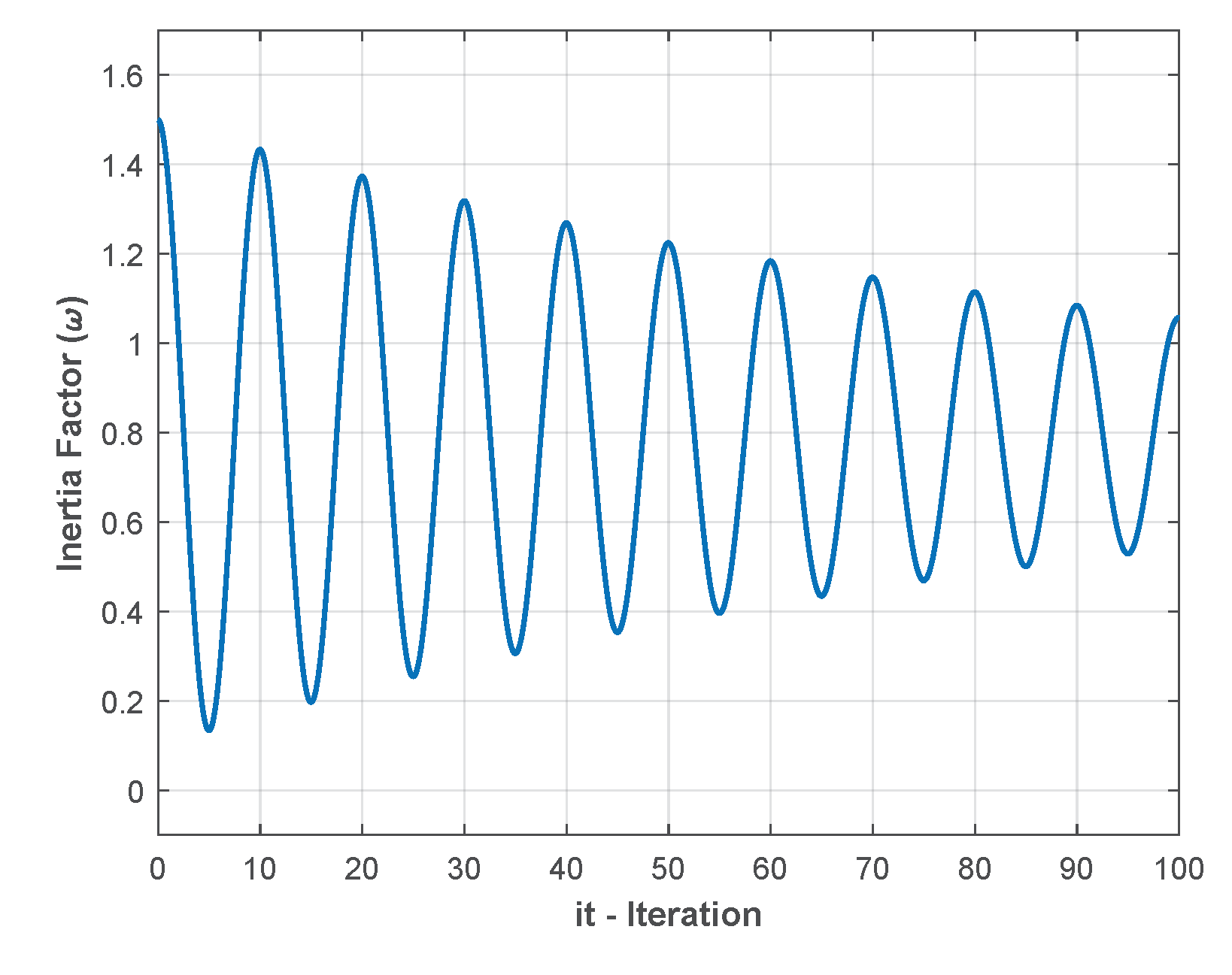
In this algorithm, the inertial weight factor

ω

operates with a decreasing cosine function, which then increases and decreases again periodically, as the number of iterations increases. The inertial weight factor

ω

of the PSO - POED algorithm is calculated by:

ω = [c o s (\frac{2 . π . i t e r}{c y c l e s}) . m . E_{d}] + S

(15)

Where iter is the current iteration, cycles is the number of iterations necessary to complete the period, M is the period of the signal,

E_{d}

is the amplitude of the signal and S is the displacement function, which allows the function

ω

along the y-axis of the Cartesian plane.

The variables

E_{d}

and S are calculated by:

E_{d} = e^{\frac{M . E_{t} - i t e r}{θ}}

(16)

S = (m + ω_{m i n})

(17)

E_{t} = i n t (i t e r / M)

(18)

Where: int(X), is the integer part of X.

M represents the period of the oscillation, while

θ

is the factor that multiplies the amplitude of said oscillation.

Obtaining m by:

m = \frac{(ω_{m a x} - ω_{m i n})}{2}

(19)

Figure 7 shows the behavior of the inertial weight factor of the proposed PSO - POED optimization algorithm.

Figure 8 shows the flow chart corresponding to the proposed PSO - POED optimization algorithm.

5.1. Algorithm of the Proposed Method PSO - POED

To apply the proposed method algorithm, the following steps must be followed:

Start;
Define the initial optimization conditions: Number of particles (N), Maximum number of iterations ( $i t e r_{m a x}$ ), Value of constants $c_{1}$ and $c_{2}$ ;
Define the parameter values of the inertial weight factor ( $ω$ ) of the proposed PSO - POED optimization algorithm: Number of iterations necessary to complete the period (cycles), signal period (M) and signal amplitude ( $E_{d}$ ).
Specify the lower and upper bounds of the variables;
Initialize randomly the position ( $x_{i}$ ) and velocity ( $v_{i}$ ) of the particles for each variable, respecting the lower and upper bounds for ( $x_{i}$ ) and ( $v_{i}$ );
Calculate the objective function for each particle, the $P_{b e s t}$ is the objective function for each particle, while $G_{b e s t}$ will be the best objective function value among the particles.
iteration = iteration + 1;
Updates the inertia weight factor w using Eqs. (15) to (19). The speed and position are also calculated using Eqs. (5) and (6), respectively;
Calculates the value of the objective function for each particle ( $O F_{m}$ );
Define the new $P_{b e s t}$ and $G_{b e s t}$ . If the value of $O F_{m}$ $P_{b e s t m}$ . $P_{b e s t m}$ = $O F_{m}$ . If the value of $P_{b e s t m}$ $G_{b e s t}$ . $G_{b e s t}$ = $P_{b e s t m}$ ;
Verify the stopping criteria. If it is satisfied, go to step 12, If not, go back to step 7;
The solution is obtained, $G_{b e s t}$ ;
End.

6. Simulation Results Using the PSO - POED

In this section, the proposed PSO - POED algorithm was applied to optimally tune the parameters

K_{A}

of the AVR and

K_{s t a b}

T_{1}

and

T_{2}

of the PSS of the synchronous generators of the SMIB and IEEE 9-bar test systems, keeping the values of the other parameters constant:

T_{A} = 0.02 s

T_{R} = 0.02 s

and

T_{W} = 1 s

. The results are compared with those obtained by applying the alternative optimization algorithms PSO - LD, PSO - OIW and PSO - OED. The following simulation parameters were used in all algorithms: Maximum number of iterations = 100,

w_{m a x} = 1.5

w_{m i n} = 0.1

c_{1} = 0.5

c_{2} = 1.5

and

β = 0.005

. Regarding the number of particles, for the Infinite Bar Machine System (SMIB) 50 particles were used, while for the IEEE 9-bar System 100 particles were used.

6.1. Case Study of the Single - Machine Infinite - Bus System

This system is made up of a thermoelectric generator G1, as shown in Figure 9.

In this system, a three - phase short circuit disturbance occurs on the line L1 at 50%. This disturbance that starts at the instant of 1 second and clears after 100 ms, causes the voltage drop produced by the generator G1, which is attempted to be restored by using the AVR and PSS controllers, whose selected parameters will be optimally tuned. Table 1 shows the upper and lower limits of the parameters to be determined.

For the Single - Machine Infinite - Bus system, when using the proposed PSO - POED algorithm, the best values found for the

ω

parameters are:

Cycles = 2,

θ

= 20, M = 50

Figure 10 shows the Time Response Analysis of the voltage signal of the generator G1 after the short circuit disturbance for the best and worst simulation respectively. The signal voltage was corrected by the action of the proposed PSO - POED, the voltage at the terminals of the generator G1 is the Set Point.

The values of the best and worst simulation are shown in Table 2 and Table 3 respectively, in which it can be seen that the proposed PSO - POED algorithm obtains a better average of the objective function and lower standard deviation than the alternative algorithms.

6.2. Case Study of the 9-Bus Multi-Machine System

This system is made up of three synchronous hydraulic generators: G1 (slack), G2 and G3, as seen in Figure 11.

Generators G2 and G3 produce a voltage at their terminals of 1.025 p.u and 1.026 p.u respectively. In the 9-bar IEEE System, a disturbance occurs in the first second of operation, which is cleared after 100 ms. This disturbance consists of a short circuit near the line L5-7, which produces an increase in current and a drop in voltage of the generators. By action of the controllers, this voltage level is brought back in 1ms to the voltage values produced prior to the disturbance. However, some oscillations occur in this recovery, which need to be corrected in the best way to avoid damage to the Power System, which is achieved through adequate tuning of the AVR and PSS parameters.

For the IEEE 9-bar System, when using the proposed PSO - POED algorithm, the best values found for the

ω

parameters are:

Cycles = 4,

θ

= 10, M = 20

Figure 12 shows the Time Response Analysis of the voltage signal of the generator G2 after the short circuit disturbance, which was corrected by the action of the proposed PSO - POED algorithm with which the controller parameters were tuned. The Set Point is the voltage at the terminals of the generator G2.

Figure 12 shows that the maximum peak of the voltage signal corrected by the proposed PSO - POED algorithm is 1.046 p.u., therefore the maximum overshoot (

M_{p}

) is:

M_{p} = 1.046 p . u - 1.025 p . u = 0.0210 p . u

(20)

Similarly:

M_{p} (%) = (\frac{1.046 - 1.025}{1.025}) * 100 % = 2.05 %

(21)

Additionally, it is observed that the signal keeps into the error band since the second peak, whose value is 1.0362. The steady state error (

E_{s s}

) is the difference between this value and the set point (1.025), giving the value of 0.0112%.

In Figure 12 the lower dashed red line marks 10% of the final value, while the upper dashed red line marks 90% of the final value. Once these values have been identified, it follows that the rise time (

t_{r}

) of the signal is 0.2617s, since this value is the difference between the instant in which the signal crosses the set point and the time at which the signal appears.

The admissible tolerance to consider that the system is in steady state is assigned to 2%, therefore the band that indicates that the response signal remains in this state is defined by the upper limit (

u_{l}

) and lower limit (

l_{l}

), as seen in Figure 12, which are obtained according to:

u_{l} = 1.025 + (0.02) (1.025) = 1.0455

(22)

l_{l} = 1.025 - (0.02) (1.025) = 1.0045

(23)

Knowing these values, the settling time (

t_{s}

) of the response signal is 0.3017s because this value is the difference between the time in which the signal enters and remains within the error band, which occurs in the second peak, and the emergence of the signal.

Similarly, alternative algorithms variants of the classic PSO were applied in order to evaluate their performance and compare the results obtained with the proposed algorithm. Figure 13 shows the response signals to the disturbance applying the alternative algorithms and the proposed PSO - POED algorithm.

Figure 13 shows that the signal of the proposed PSO - POED algorithm is the fastest, since it reaches the reference first, so its rise time (

t_{r}

) is the shortest among the four algorithms. Likewise, it is observed that the signal of the proposed PSO - POED algorithm presents the lowest maximum overshoot value (

M_{p}

), the shortest settling time (

t_{s}

) and the lowest steady state error (

E_{s s}

)

In a similar way, this analysis is carried out for the G3 generator of the 9-Bus Multi -Machine Power System. Figure 14 shows the Time Response Analysis of the voltage signal of the generator G3 after the short circuit disturbance, which was corrected by the action of the proposed PSO - POED algorithm with which the parameters of its controllers were tuned.

Figure 14 shows that the maximum peak of the voltage signal corrected by the proposed PSO - POED algorithm is 1.047 p.u., therefore the maximum overshoot (

M_{p}

) is:

M_{p} = 1.047 p . u - 1.026 p . u = 0.0210 p . u .

(24)

Similarly:

M_{p} (%) = (\frac{1.047 - 1.026}{1.026}) * 100 % = 2.05 %

(25)

Additionally, it is observed that the steady state error (

E_{s s}

) is: 0.0077%.

Similarly, in Figure 14 the lower red dashed line marks 10% of the final value, while the upper dashed red line marks 90% of the final value. Once these values have been identified, it follows that the growth time (

t_{r}

) of the signal is 0.242s.

Considering 2% as the admissible tolerance value for the system to be in steady state, the upper (

l_{s}

) and lower (

l_{i}

) limits are calculated according to:

l_{s} = 1.026 + (0.02) (1.026) = 1.0465

(26)

l_{i} = 1.026 - (0.02) (1.026) = 1.0055

(27)

Knowing these values, the settling time (

t_{s}

) of the response signal is 0.2817s.

Similarly, alternative algorithms variants of the classic PSO were applied in order to evaluate their performance and compare the results obtained with the proposed algorithm. Figure 15 shows the response signals to the disturbance applying the alternative algorithms and the proposed PSO - POED algorithm.

Figure 15 shows that the signal of the proposed PSO - POED algorithm is the fastest, since it reaches the reference first, so its growth time (

t_{r}

) is the shortest among the four algorithms. Likewise, it is observed that the signal of the proposed PSO - POED algorithm presents the lowest maximum overshoot value (

M_{p}

), the shortest settling time (

t_{s}

) and the lowest steady state error (

E_{s s}

The parameters of the AVR and PSS controllers are tuned to values within established ranges. These limits for both controllers are shown in Table 4.

Table 4 shows that the established limits are different from those indicated in Table 1, this is because the SMIB System has a thermoelectric generator, while in the 9-bar IEEE System the generators are hydraulic.

Table 5 shows the AVR and PSS parameters obtained by applying the proposed algorithm and the alternative algorithms, which were also applied in this paper for comparison purposes. Likewise, the convergence results for the 100 simulations carried out using the different algorithms are shown.

Table 5 shows that the proposed algorithm (PSO - POED) is superior in several aspects to the alternative algorithms (PSO - LD, PSO - OIW and PSO - OED), mainly by observing the best result obtained from the 100 simulations (Best), as well as the worst and the average result (Worst and Average, respectively), which turns out to be greater than the others. The value of the standard deviation (Stand.Dev.) obtained by using the PSO - POED is higher than the others because the results obtained are significantly high. In fact, the worst solution found by PSO - POED far exceeds the better solutions from the other algorithms.

Table 6 shows the values of the parameters of the voltage signal of the generators in the Time Response Analysis, which were obtained by applying the different algorithms.

Table 6 shows that by applying the proposed algorithm (PSO - POED), better values are obtained for the parameters of rise time (

t_{r}

), settling time (

t_{s}

), steady state error (

E_{s s}

) and peak overshoot (

M_{p}

) than when applying the alternative algorithms (PSO - LD, PSO - OIW and PSO - OED), which is true for both synchronous generators.

7. Conclusions

In this paper, a new algorithm for the simultaneous tuning of the optimal parameters of the Automatic Voltage Regulator (AVR) and the Power System Stabilizer (PSS) using the proposed technique of the Particle Swarm Optimization with Periodic Oscillating Exponential Decay (PSO-POED) was proposed. The PSO-POED is characterized by a modification in the inertia weight factor, so that it has the form of an oscillatory function with periodic exponential decay. This modification aims to provide an improvement in the search quality of the optimum point for tuning the parameters. Thus, the proposed method shall be a potentially efficient and robust alternative for simultaneous tuning of the parameters of AVR and PSS.

Declaration of Competing Interest

The authors declare that they have no known competing financial interests or personal relationships that could have appeared to influence the work reported in this paper.

References

Kundur, P. Power system stability. Power system stability and control 2007, 10, 7–1. [Google Scholar]
Saadat, H.;others. Power systemanalysis; Vol.2,McGraw-hill,1999.
Costa Filho, R.N.D.; Paucar, V.L. Robust coordinated design of AVR+ PSS using quantum particle swarm optimization. ITEGAM-JETIA 2020, 6, 15–20. [Google Scholar] [CrossRef]
Rodrigues, F.; Molina, Y.; Silva, C.; Naupari, Z. Simultaneous tuning of the AVR and PSS parameters using particle swarm optimization with oscillating exponential decay. International Journal of Electrical Power & Energy Systems 2021, 133, 107215. [Google Scholar]
Marić, P.; Kljajić, R.; Chamorro, H.R.; Glavaš, H. Power system stabilizer tuning algorithm in a multimachine system based on S-domain and time domain system performance measures. Energies 2021, 14, 5644. [Google Scholar] [CrossRef]
Salesi-Mousaabadi, M.; Shahgholian, G. Simultaneous adjustment of AVR and optimized PSS outputs effect in power systems for stability improvement. Journal of Power Technologies 2023, 103. [Google Scholar]
Rodrigues, F.; Molina, Y.; Araujo, C. Simultaneous tuning of AVR and PSS using particle swarm optimization with two stages. IEEE Latin America Transactions 2020, 18, 1623–1630. [Google Scholar] [CrossRef]
Selvabala, B.; Devaraj, D. Co-ordinated design of AVR-PSS using multi objective genetic algorithm. Swarm, Evolutionary, and Memetic Computing: First International Conference on Swarm, Evolutionary, and Memetic Computing, SEMCCO 2010, Chennai, India, December16-18, 2010. Proceedings 1. Springer, 2010, pp. 481–493. 16 December.
Selvabala, B.; Devaraj, D. Co-ordinated tuning of AVR-PSS using differential evolution algorithm. 2010 Conference Proceedings IPEC. IEEE, 2010, pp. 439–444.
Manuaba, I.; Abdillah, M.; Priyadi, A.; Purnomo, M.H. Coordinated tuning of PID-based PSS and AVR using bacterial foraging-PSOTVAC-DE algorithm. Control and Intelligent Systems 2015, 43, 1–9. [Google Scholar] [CrossRef]
Usman, J.; Mustafa, M.W.; Aliyu, G. Design of AVR and PSS for power system stability based on iteration particle swarm optimization. International Journal of Engineering and Innovative Technology (IJEIT) 2012, 2. [Google Scholar]
Nirmal, J.F.; Auxillia, D.J. Adaptive PSO based tuning of PID controller for an Automatic Voltage Regulator system. 2013 International Conference on Circuits, Power and Computing Technologies (ICCPCT). IEEE, 2013, pp. 661–666.
Špoljarić, T.; Pavić, I.; Alinjak, T. Performance Comparison of No-preference and Weighted Sum Objective Methods in Multi-Objective Optimization of AVR-PSS Tuning in Multi-machine Power System. Tehnički vjesnik 2022, 29, 1931–1940. [Google Scholar]
Mitra, P.; Chowdhury, S.; Chowdhury, S.; Pal, S.; Crossley, P. Intelligent AVR and PSS with Adaptive hybrid learning algorithm. 2008 IEEE Power and Energy Society General Meeting-Conversion and Delivery of Electrical Energy in the 21st Century. IEEE, 2008, pp. 1–7.
Khezri, R.; Bevrani, H. Fuzzy-based coordinated control design for AVR and PSS in multi-machine power systems. 2013 13th Iranian Conference on Fuzzy Systems (IFSC). IEEE, 2013, pp. 1–5.
Rodrigues, F.W. ; others. Projeto simultâneo do regulador automático de tensão e estabilizador de sistema de potência utilizando otimização por enxame de partículas modificado 2019.
Silva Junior, J.N.R.d. Sintonia ótima de regulador automático de tensão e estabilizador de sistema de potência utilizando algoritmo de otimização por enxame de partículas 2012.

Figure 1. Single machine-infinite bus-system.

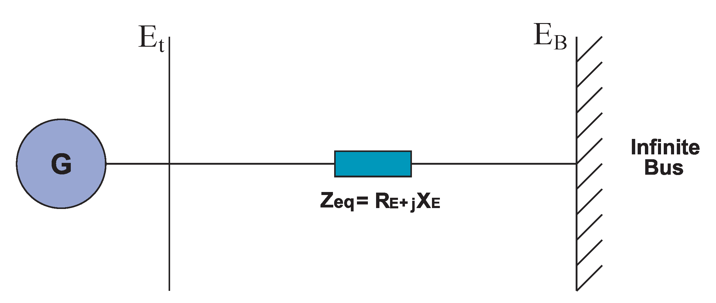
Figure 2. Block diagram of a Synchronous Generator with an AVR and PSS.

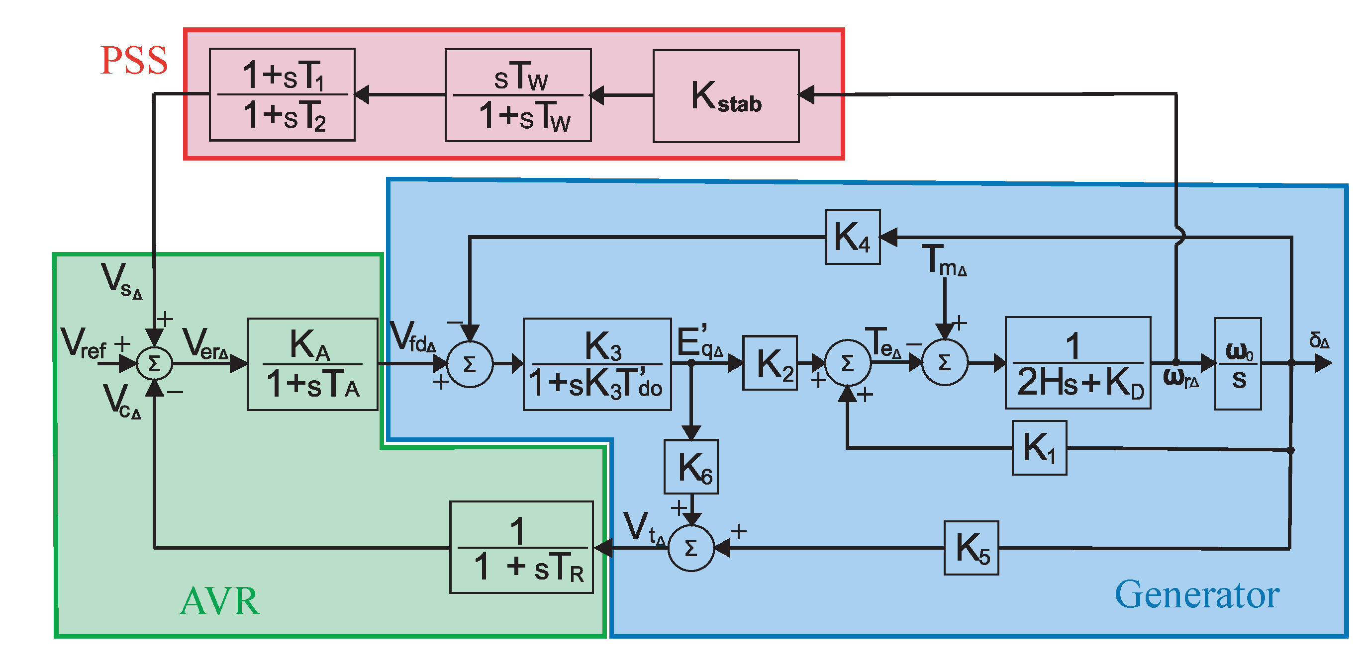
Figure 3. Typical response signal of an underdamped system to a test signal and its performance parameters.

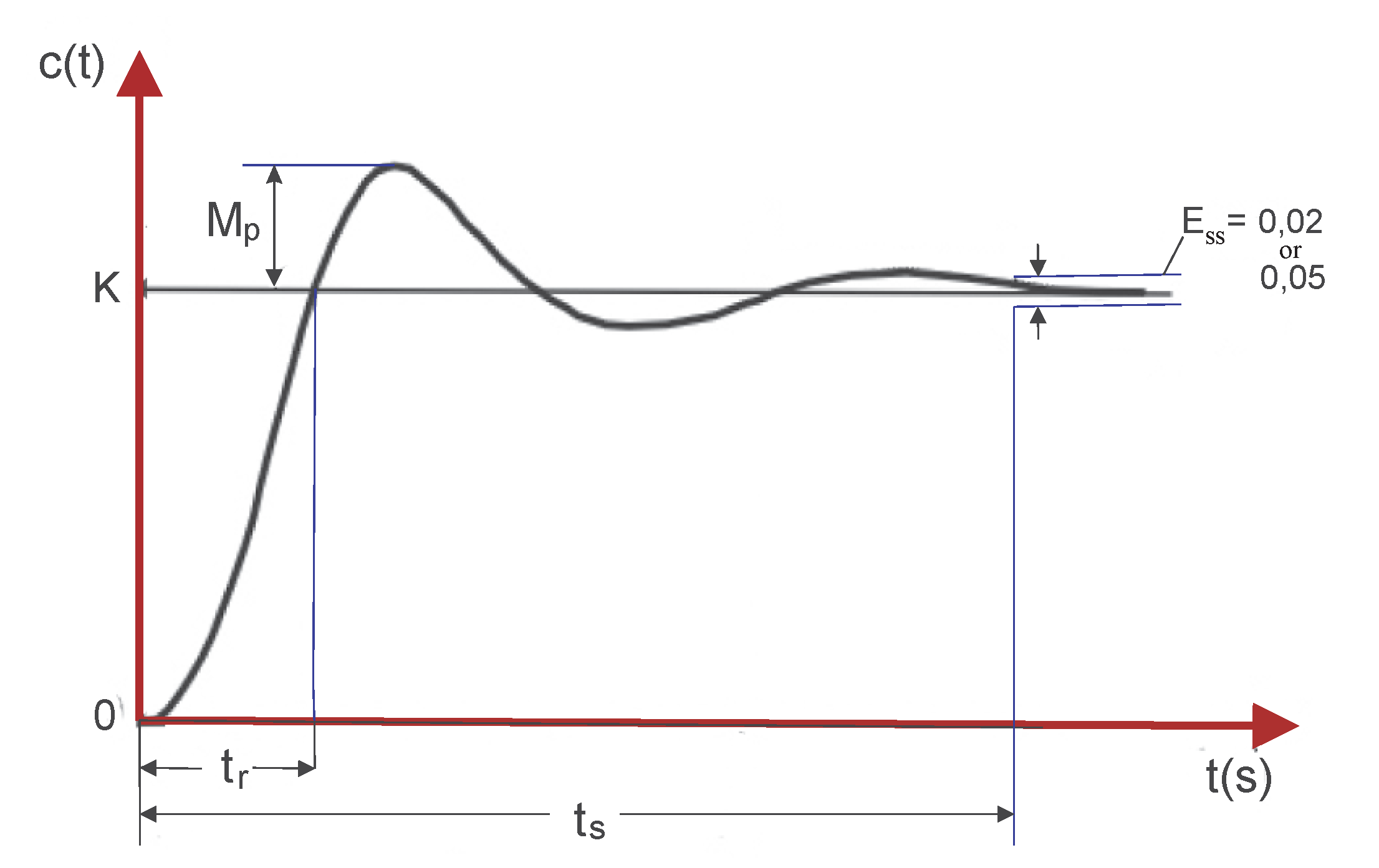
Figure 4. Inertia weight factor for PSO - LD.

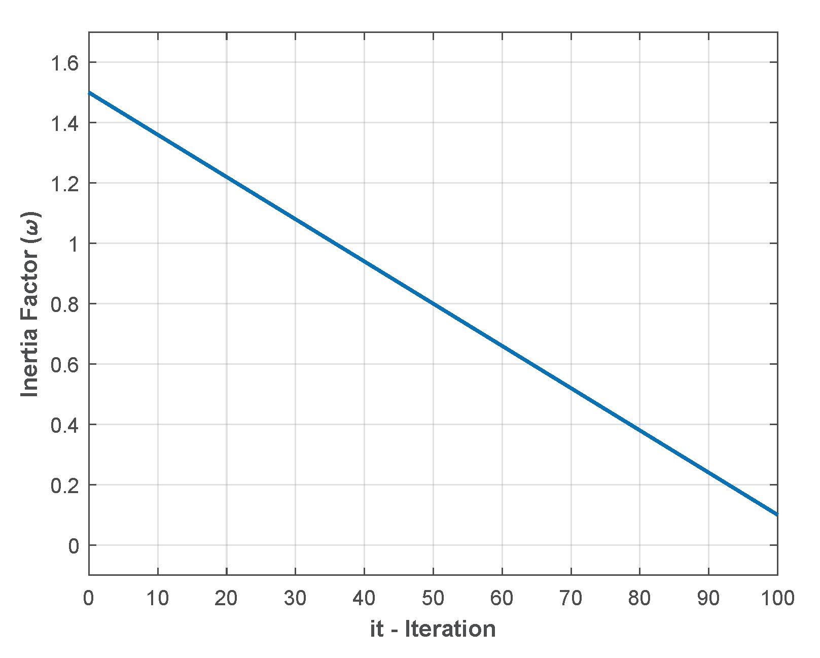
Figure 5. Inertia weight factor for PSO - OIW.

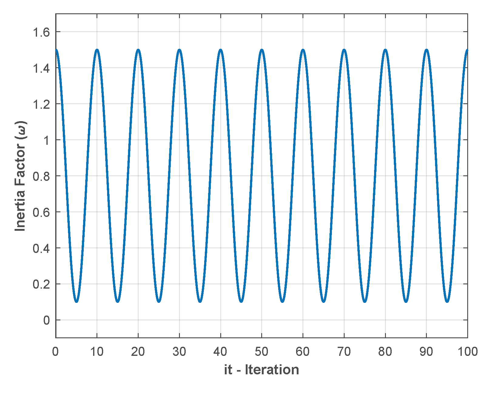
Figure 7. Inertial weight factor for PSO - POED.

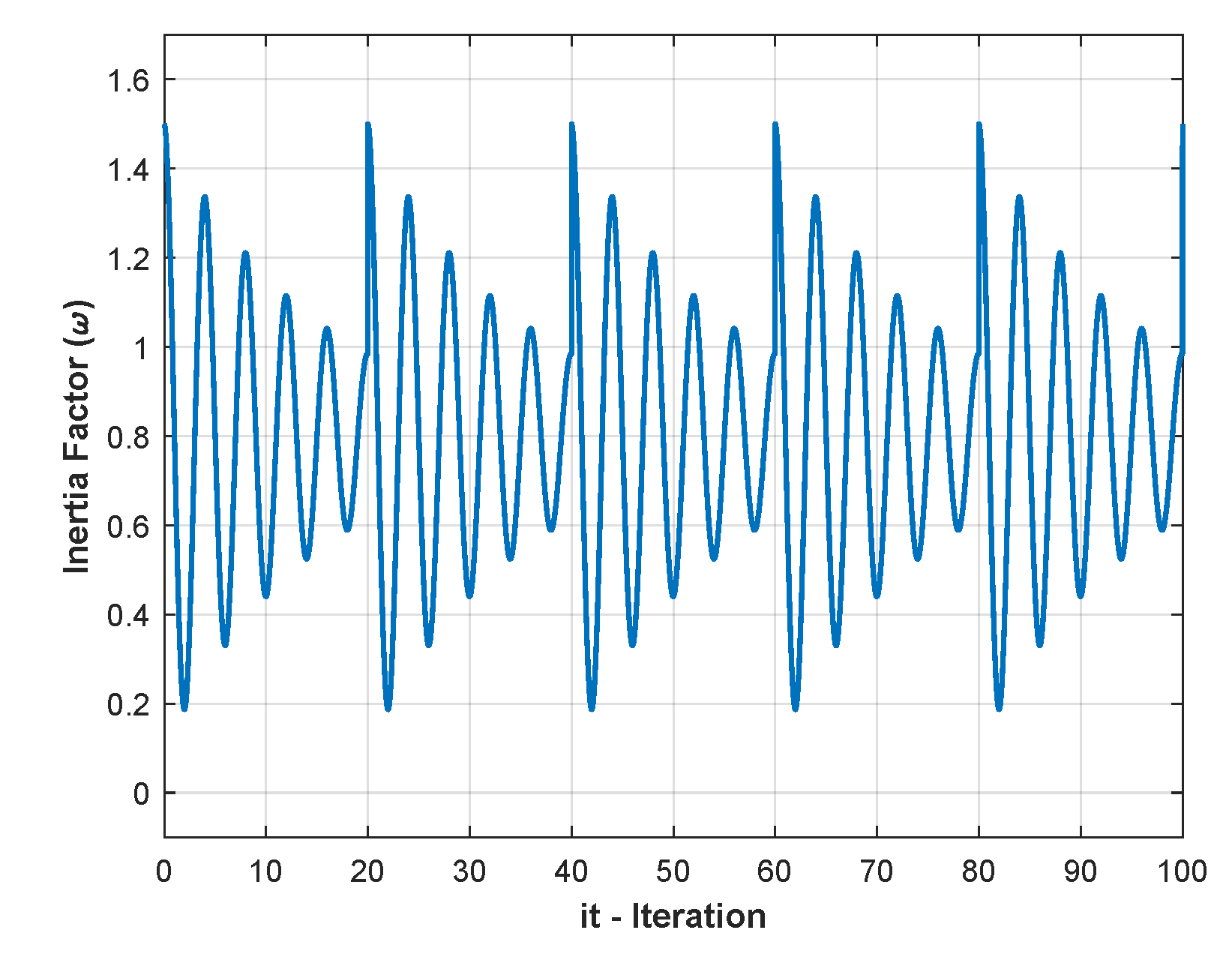
Figure 8. Flowchart of the proposed optimization algorithm PSO - POED.

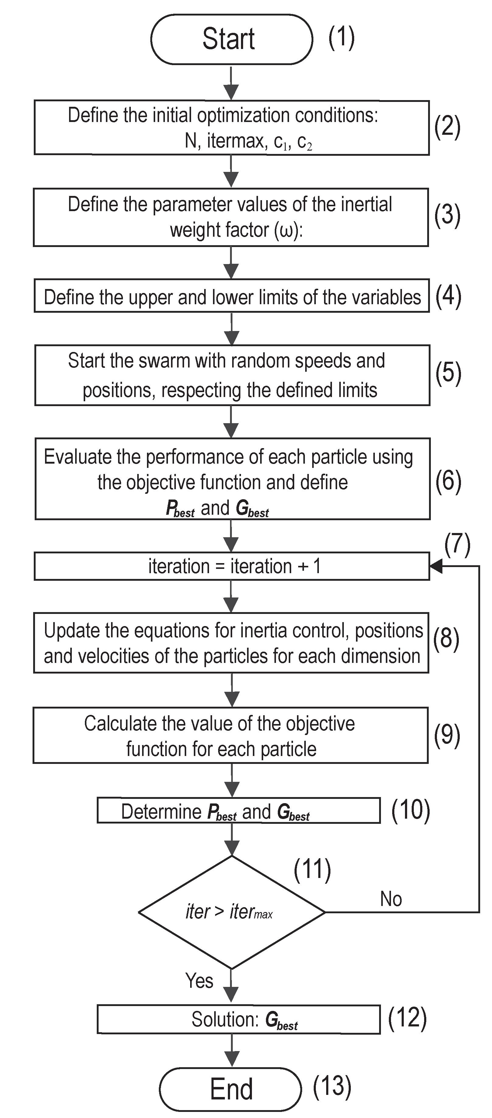
Figure 9. System used for SMIB.

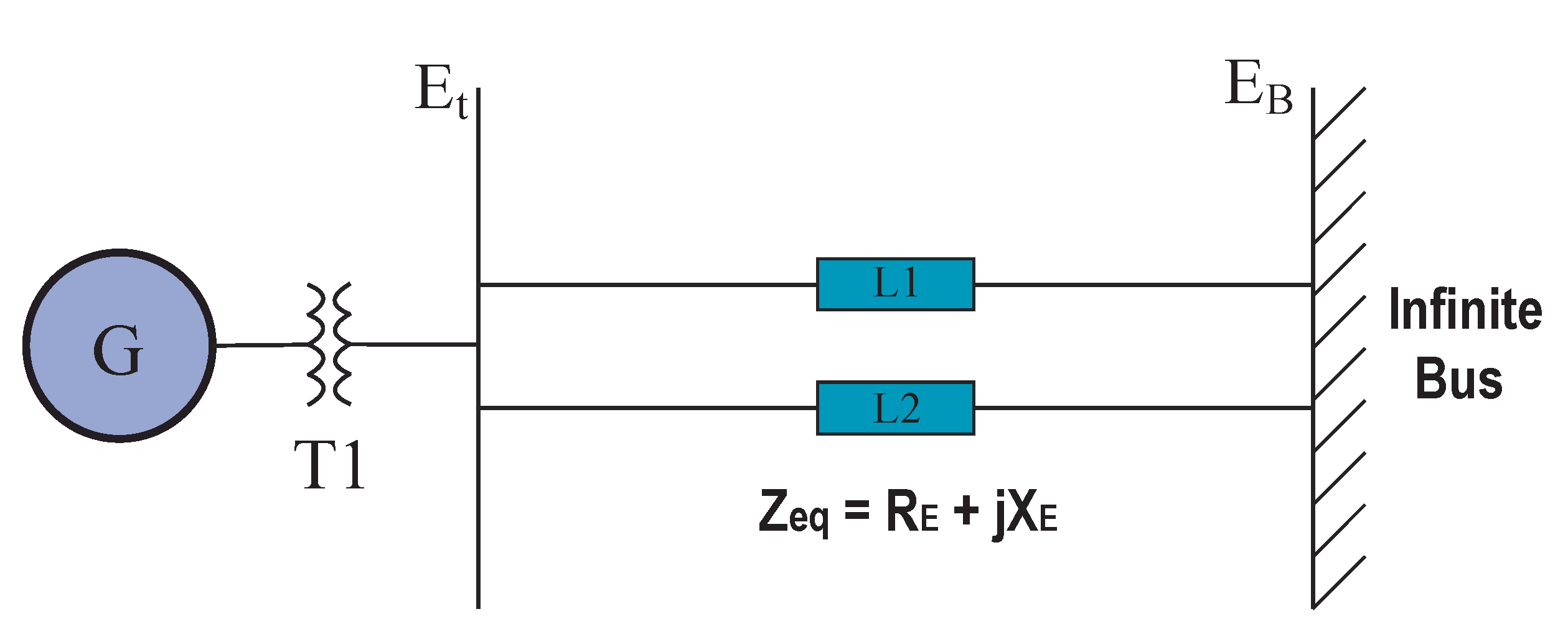
Figure 10. Comparison of methods for SMIB

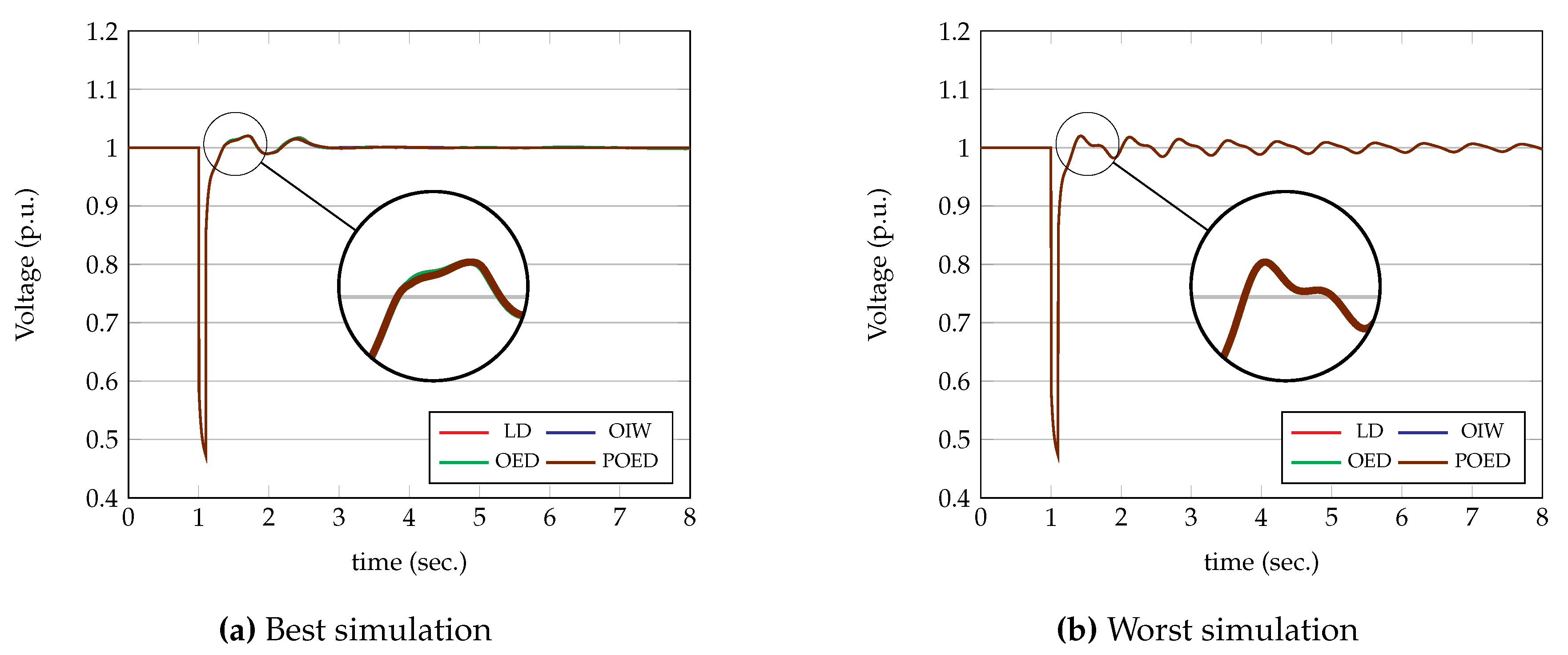
Figure 11. 9-Bus Multi-Machine System.

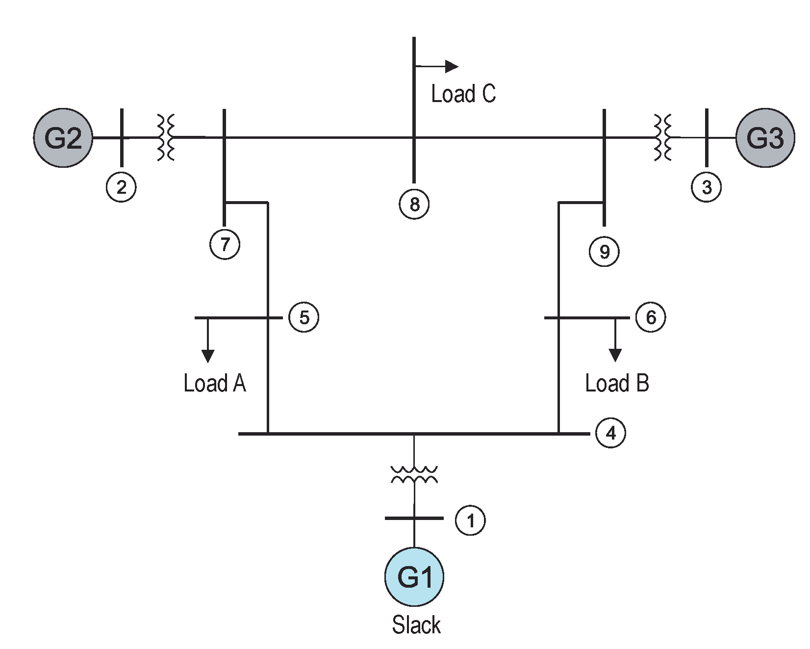
Figure 12. POED for 9 buses - G2 - Best

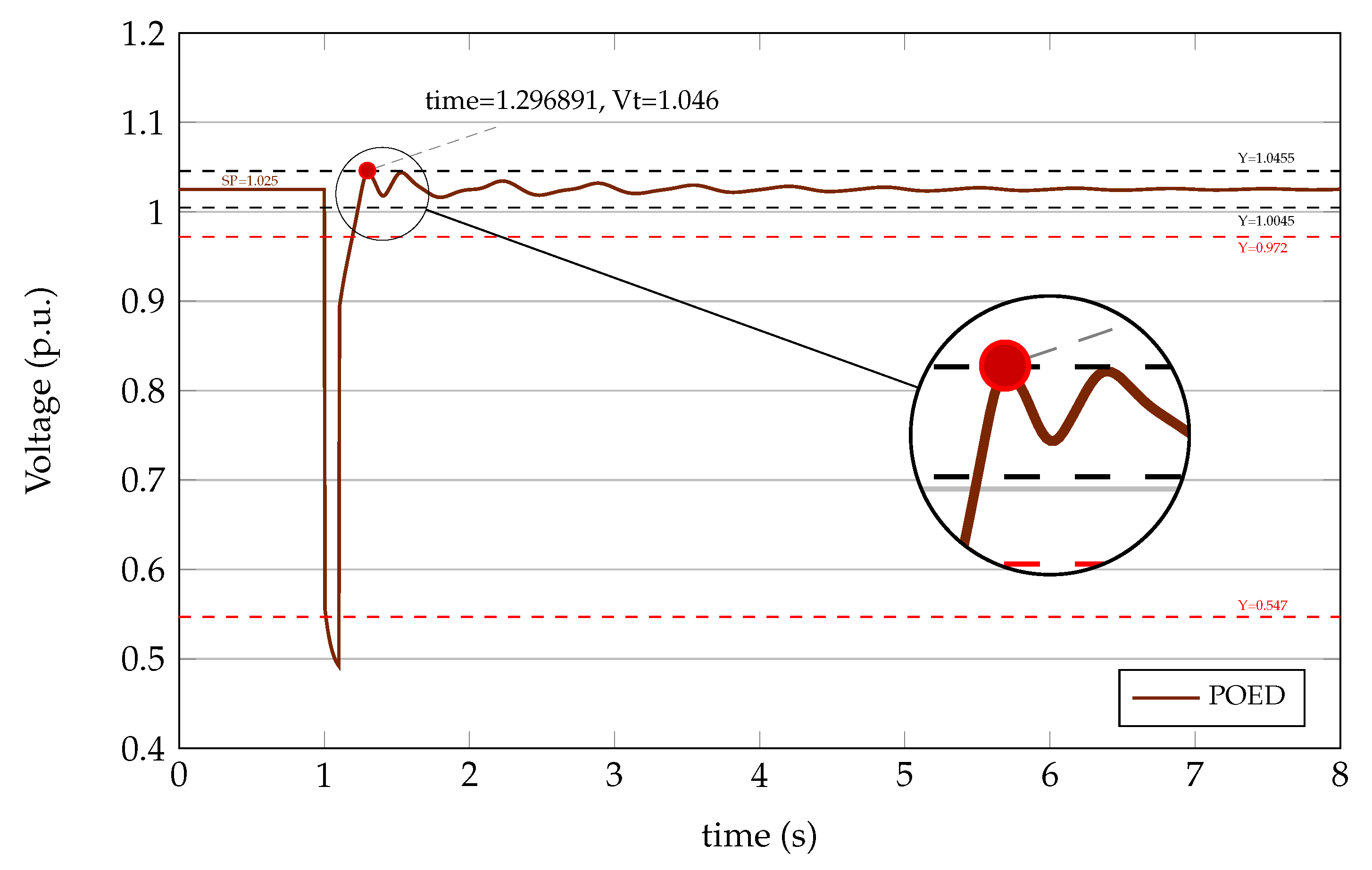
Figure 13. Comparison of methods for 9 buses - G2 - Best

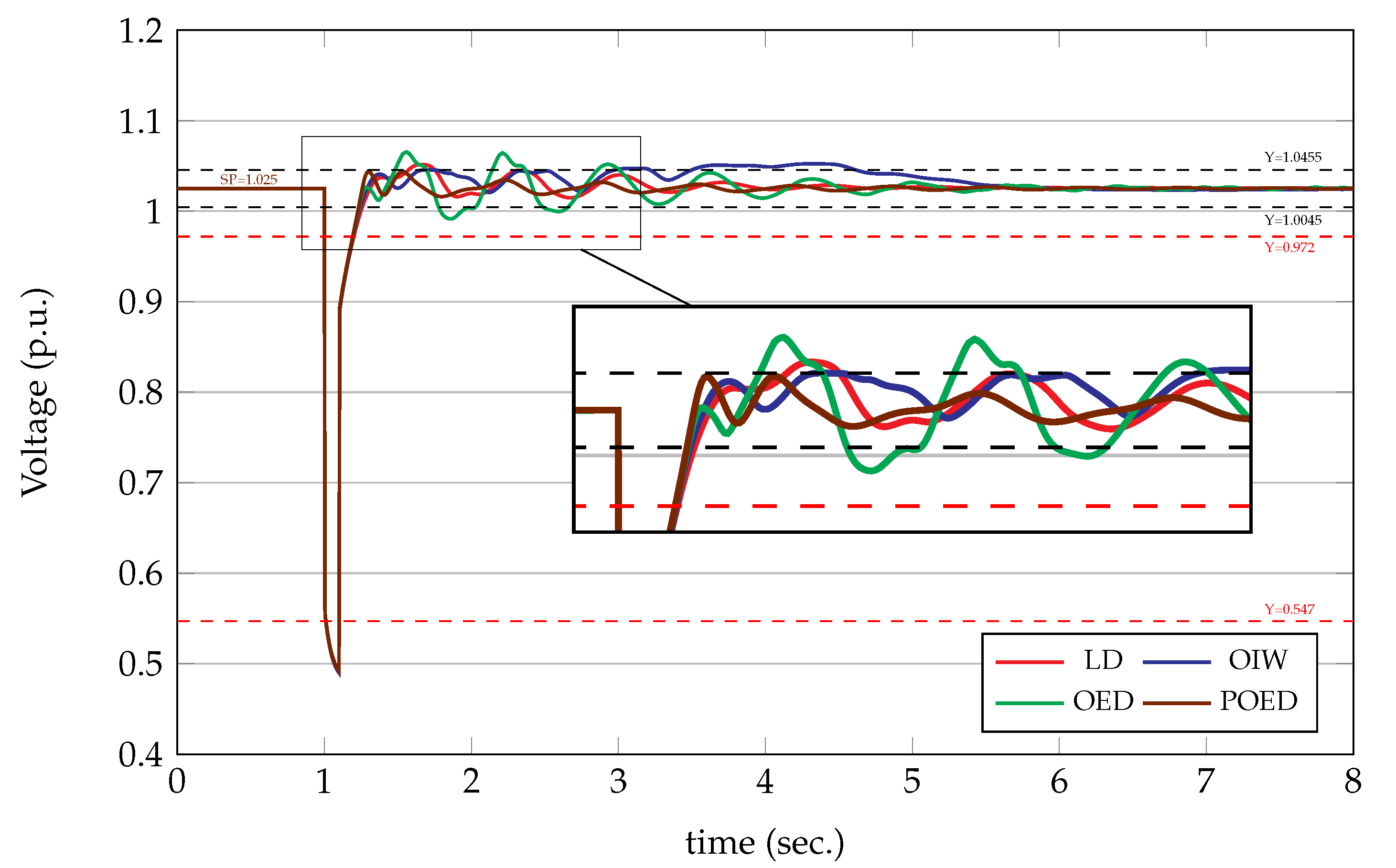
Figure 14. POED for 9 buses - G3 - Best

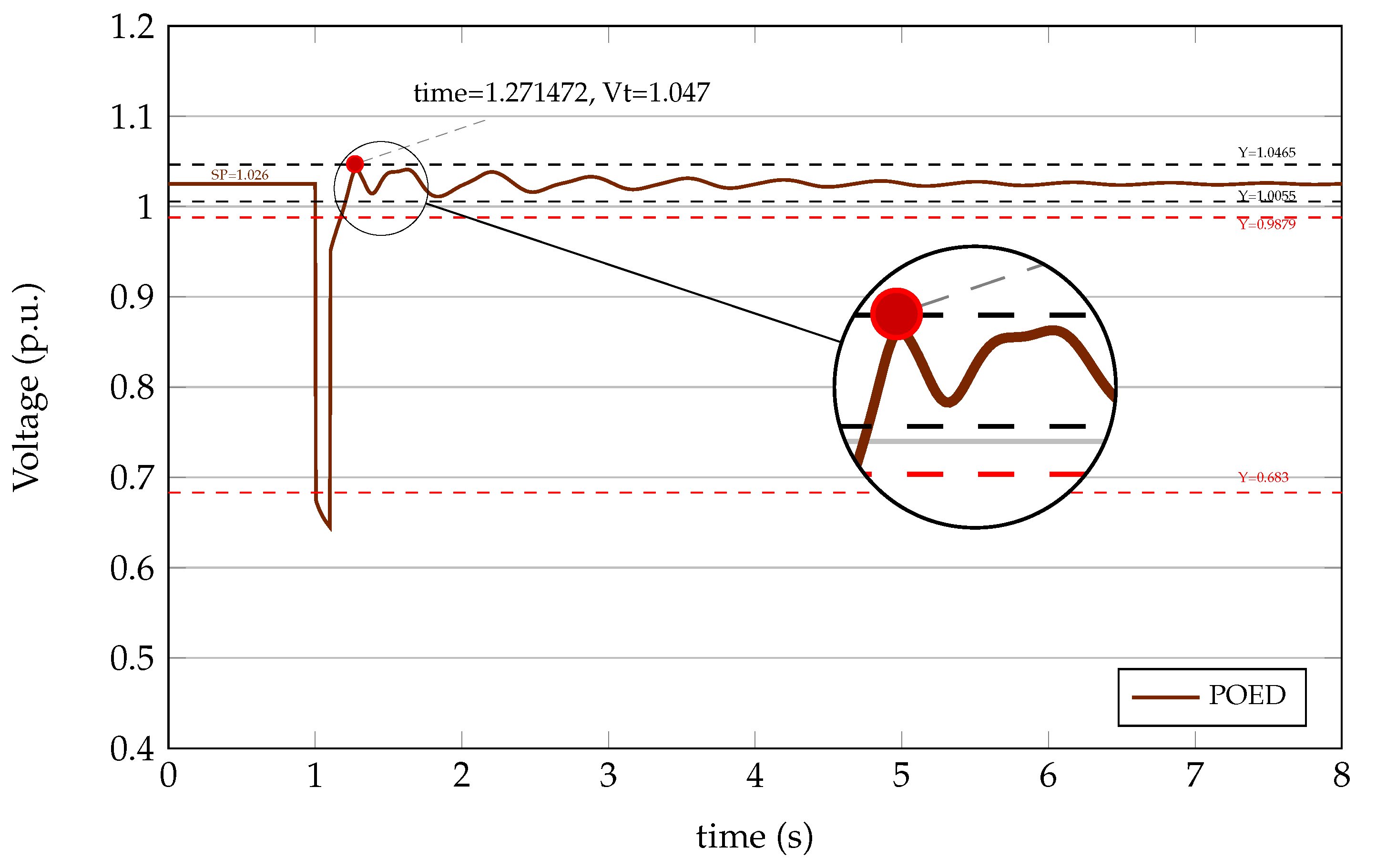
Figure 15. Comparison of methods for 9 buses - G3 - Best

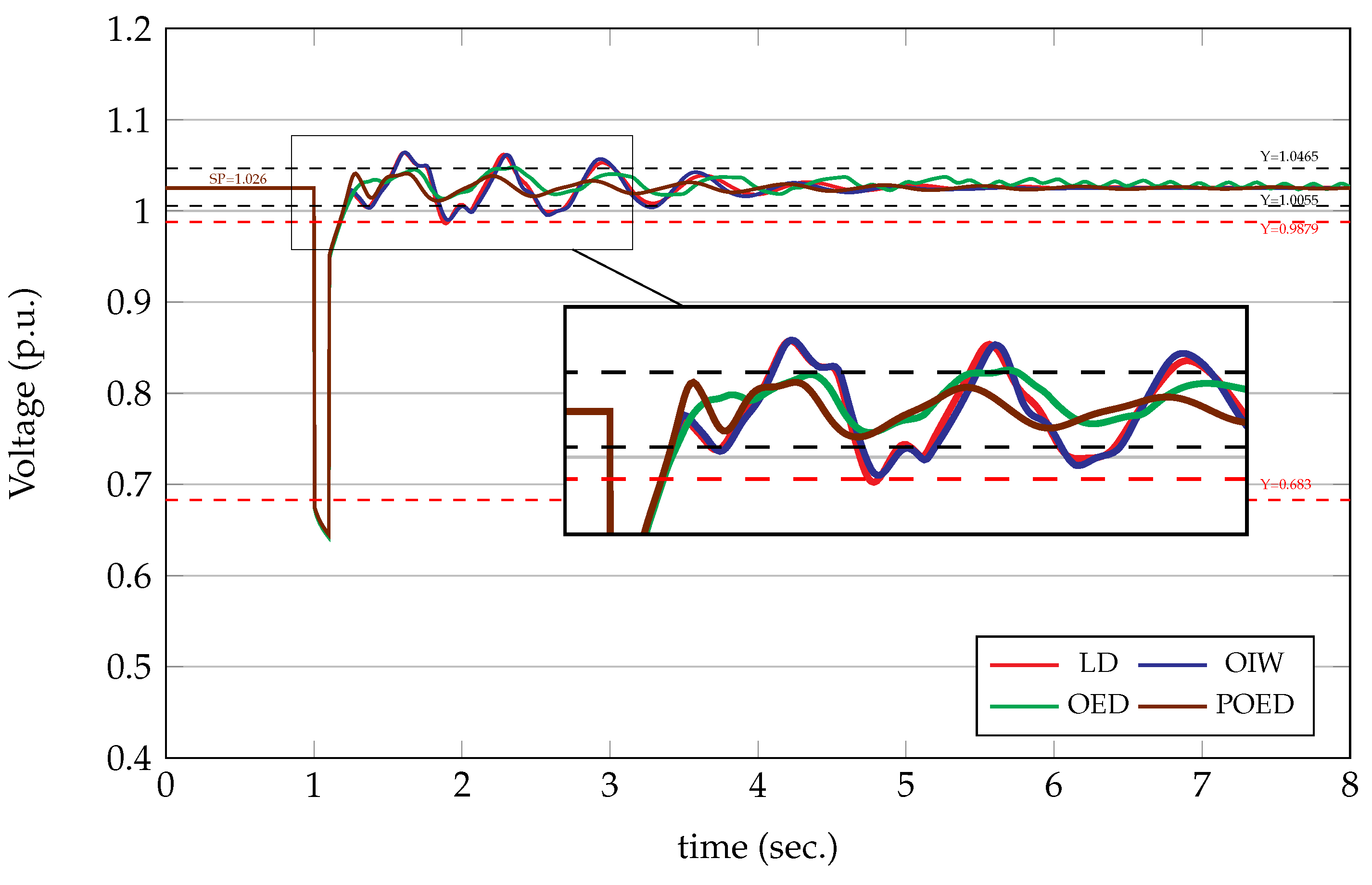
Table 1. Upper and lower limits of the parameters of the AVR and PSS of the SMIB.

Parameters	$K_{A} (p . u .)$	$K_{s t a b} (p . u .)$	$T_{1} (s)$	$T_{2} (s)$
Upper limit	400	2	3	0.5
Lower limit	1	0.1	1	0.0001

Table 2. AVR and PSS parameters obtained by applying the different algorithms.

	Solution					Objective Function
Algorithm		$K_{A}$ (p.u)	$K_{s t a b}$ (p.u)	$T_{1}$ (s)	$T_{2}$ (s)	Stand.Dev.	Average	Best	Worst
PSO-LD	Best	124.06	0.1	1	0.5	2.367	5.259	9.934	2.791
	Worst	100.47	2	3	0.0001
PSO-OIW	Best	124.06	0.1	1	0.5	2.118	5.031	9.934	2.791
	Worst	104.68	1.92	1	0.0001
PSO-OED	Best	124.06	0.1	1	0.5	2.220	5.220	9.934	2.791
	Worst	100.19	1.62	3	0.0001
Proposed	Best	124.06	0.1	1	0.5	2.108	5.305	9.934	2.791
PSO-POED	Worst	109.36	2	1.54	0.0102

Table 3. Time Response parameters obtained by applying the different algorithms.

	Best Solution				Worst Solution
Algorithm	$t_{r}$ (s)	$t_{s}$ (s)	$E_{s s}$ (%)	$M_{p}$ (%)	$t_{r}$ (s)	$t_{s}$ (s)	$E_{s s}$ (%)	$M_{p}$ (%)
PSO-LD	0.332	0.422	0.229	2.0	0.352	0.702	0.0000	2.0
PSO-OIW	0.332	0.422	0.229	2.0	0.352	0.702	0.0002	2.0
PSO-OED	0.332	0.422	0.229	2.0	0.352	0.702	0.0002	2.0001
PSO-POED	0.332	0.422	0.229	2.0	0.352	0.702	0.0004	2.0

Table 4. IEEE 9-Bar System AVR and PSS Parameter Limits.

Parameters	$K_{A} (p . u .)$	$K_{s t a b} (p . u .)$	$T_{1} (s)$	$T_{2} (s)$
Upper limit	400	50	1	0.05
Lower limit	1	0.1	0.6	0.005

Table 5. AVR and PSS parameters obtained by applying the different algorithms.

	Best Solution					Objective Function
Algorithm	Generator	$K_{A}$ (p.u)	$K_{s t a b}$ (p.u)	$T_{1}$ (s)	$T_{2}$ (s)	Stand.Dev.	Average	Best	Worst
PSO-LD	$G_{2}$	37.29	1.2197	1	0.0356	0.6917	13.9374	14.1578	12.0357
	$G_{3}$	400	1	1	0.0261
PSO-OIW	$G_{2}$	39.75	49.1465	0.0868	0.0489	0.4835	14.1358	14.5754	13.7565
	$G_{3}$	400	1	1	0.0305
PSO-OED	$G_{2}$	400	1	0.6001	0.0050	0.1208	14.5941	14.7762	14.0978
	$G_{3}$	34.77	50	1	0.0470
Proposed	$G_{2}$	400	0.1038	1	0.0271	4.1126	35.9307	39.9424	20.1955
PSO-POED	$G_{3}$	400	0.1457	1	0.0464

Table 6. Parameters of the voltage signal in the Time Response Analysis of both generators using the different algorithms.

Algorithm	Generator	Terminal Voltage
		$t_{r}$ (s)	$t_{s}$ (s)	$E_{s s}$ (%)	$M_{p}$ (%)
PSO-LD	$G_{2}$	1.1417	1.2517	2.5856	4.4956
PSO-OIW	$G_{2}$	1.1517	1.2517	3.0245	4.3509
PSO-OED	$G_{2}$	1.1416	1.2417	2.5890	3.9360
Proposed PSO-POED	$G_{2}$	0.2617	0.3017	0.0112	2.0500
PSO-LD	$G_{3}$	1.1050	1.2117	2.3702	4.0054
PSO-OIW	$G_{3}$	1.1050	1.2117	2.3655	4.0567
PSO-OED	$G_{3}$	1.1050	1.2117	2.6455	3.9099
Proposed PSO-POED	$G_{3}$	0.2417	0.2817	0.0077	2.0500

Disclaimer/Publisher’s Note: The statements, opinions and data contained in all publications are solely those of the individual author(s) and contributor(s) and not of MDPI and/or the editor(s). MDPI and/or the editor(s) disclaim responsibility for any injury to people or property resulting from any ideas, methods, instructions or products referred to in the content.

© 2024 by the authors. Licensee MDPI, Basel, Switzerland. This article is an open access article distributed under the terms and conditions of the Creative Commons Attribution (CC BY) license (http://creativecommons.org/licenses/by/4.0/).

Copyright: This open access article is published under a Creative Commons CC BY 4.0 license, which permit the free download, distribution, and reuse, provided that the author and preprint are cited in any reuse.

Downloads

115

Views

Comments

Subscription

Notify me about updates to this article or when a peer-reviewed version is published.

MDPI Initiatives

Important Links

Choose an area of interest and we will send you notifications of new preprints at your preferred frequency.

Disclaimer

Simultaneous Tuning of the AVR and PSS Parameters Using Particle Swarm Optimization with Periodic Oscillating Exponential Decay

Abstract

Keywords:

Subject:

1. Introduction

2. Linearized Model of a Single-Machine Infinite-Bus System

3. Simultaneous Tuning of AVR and PSS Parameters

4. Particle Swarm Optimization - PSO

4.1. PSO with Linear Decay (PSO - LD)

4.2. PSO with Oscillating Inertia Weight (PSO - OIW)

4.3. PSO with Oscillating Exponential Decay (PSO - OED)

5. Proposed Method

5.1. Algorithm of the Proposed Method PSO - POED

6. Simulation Results Using the PSO - POED

6.1. Case Study of the Single - Machine Infinite - Bus System

6.2. Case Study of the 9-Bus Multi-Machine System

7. Conclusions

References

MDPI Initiatives

Important Links

Subscribe