1. Introduction
Recent developments in quantum computing have enabled the application of machine learning paradigms within a quantum framework [
1,
2]. This innovative field leverages quantum physics principles, like entanglement, superposition, and interference, to execute computational loads [
3,
4]. With these properties, it is theorized that quantum computers can leverage computational time in critical areas, such financial transactions decisions, new materials and drugs discovery, cryptography, and so on [
5]. Unlike classical computers, quantum computers process information using quantum bits (qubits). The qubit’s state, represented by its orientation in a high-dimensional complex Hilbert ℂ
⊗n space (being n the number of qubits), is managed by quantum gates. These unitary operators perform reversible operations on qubits, altering their orientation within the Hilbert space. These operations can implement superposition, entanglement, and interference properties to the quantum circuit, composed of qubit, allowing computers to generate unique and more complex patterns than those produced by classical computational systems. In this way, it is expected that quantum machine learning (QML) models will surpass the predictive performance of traditional ML approaches, reaching the called quantum advantage, where a complex problem can be efficiently tackled with a quantum framework [
1,
6].
Despite being a newly developed field, applications of the QML are broad and promising. One of its possible applications lies within the renewable energy area, an important player for containing the adverse effects of climate change caused by the emission of greenhouse gases. The majority of greenhouse gases come from electricity production operations [
7,
8]. Their collateral effects have been linked to damage to the ecological area [
9,
10], and the occurrence of extreme weather events [
11,
12], among other negative consequences [
13,
14]. The adverse effects of pollutant gas emissions also negatively impact the global economy, causing the loss of billions of USD worldwide [
15,
16,
17,
18].
Within this context, renewable energies pose as a major player in mitigating the harmful effects of climate change. Recently, there has been a global movement towards developing greener and renewable energy sources. One can highlight the importance of solar power, which has led the Global investments in renewable energies [
19,
20].
While renewable energies offer significant benefits in cleaner energy production, their inherently stochastic and intermittent nature presents challenges. Therefore, the development of precise and reliable tools for predicting energy output from these sources is crucial. Machine learning (ML) has emerged as a valuable tool in this regard, demonstrating its ability to identify complex relationships within time-series data, in this manner enhancing the accuracy of renewable energy forecasting. Numerous works have employed ML to assess the behavior of key environmental indicators [
21,
22,
23,
24], including renewable energy sources [
7,
25,
26,
27,
28]. However, Quantum machine learning (QML), remains in its early stages, with an absence of studies exploring its application in time-series scenarios and, consequently, in the modeling of renewable energy sources [
29,
30].
To address the knowledge gap in QML applications within renewable energy, this study proposes the development of a simulated quantum neural network (QNN) framework to forecast solar irradiance up to 3 hours in advance. The framework utilizes the benchmarking dataset from Folsom, as introduced by Pedro et al. [
31]. The main objectives of this work are as follows:
To address the information gap in the scientific literature regarding solar irradiance estimation using QML predictive models.
To assess the feasibility of a QML model designed for forecasting solar irradiance up to 3 hours in advance.
To evaluate different configurations for the QNN framework, investigating several parameters composing its structure and their impact in the model’s output.
To investigate different optimization strategies, and their impact on the model’s output.
To evaluate the QNN performance compared to classical ML counterparts.
2. Materials and Methods
2.1. Solar Irradiance
Solar irradiance touching the Earth’s surface can be categorized into three distinct types. The first type, Direct Normal Irradiance (DNI), includes all solar irradiance reaching the Earth's surface directly without dispersion. When dispersion occurs, it is referred to as diffuse irradiance (DI). The third type, Global Horizontal Irradiance (GHI), encompasses the total solar energy reaching the Earth's surface from all directions, i.e. DNI and DI included [
32].
Accurate forecasting of GHI and DNI is essential to the cost-efficient implementation of photovoltaic projects and the proper development of public policies or plans related to solar energy [
33,
34,
35].
2.2. The Folsom Dataset
The Folsom dataset spans 2014 to 2016, containing meticulously checked minute-by-minute measurements of GHI and DNI from Folsom, California, USA. This region holds elevated interest for solar irradiance given its importance on the USA economy, and its status as a technological HUB, housing millions of people [
26,
31]. The Folsom dataset was conceived to be used as a benchmark dataset to promote the development of solar forecasting models [
31], containing ground-based sky images, satellite data, and forecasts from numerical weather prediction models. For the present project, the dataset was limited to GHI and DNI measurements and sky images.
As mentioned previously, solar irradiance is stochastic and intermittent. Additionally, its forecasting depends on many factors, such as the celestial body motion, weather, geographic location, cloud coverage, and albedo, to cite a few [
25,
36]. A way to mitigate these effects, along with daily and seasonal variances of solar irradiance [
37], is using the normalization by the modelling of the clear-sky index,
, a dimensionless number comprised between 0 and 1defined as below:
In equation 1, the term
usually refers to GHI or DNI. The denominator
is a modeled value of clear-sky irradiance, representing the maximum incident irradiance reaching Earth's surface. For this dataset, the clear sky model developed by Ineichen and Perez [
38] was implemented, taking into account the characteristics of the study location.
In the original work by Pedro and colleagues [
31], from the calculated
clear-sky index value, three feature vectors were engineered, namely Backward average (B
i), Lagged average values (L
i), and the clear-sky Variability (V
i). It is important to highlight that these features are calculated within the time window preceding the desired forecasting interval. Additionally, the sky-images were collected from all sky-dome pixels, using 8-bit color images from a camera pointed toward the sky. The pixels were converted to a floating-point vector representing three different color channels: Red (R), Green (G), and Blue (B). Furthermore, the vectors relating the red-to-blue and the normalized red-to-blue ratios were also calculated. Finally, for each of the previous features, the mean value, standard deviation, and entropy were determined, resulting in fifteen features related to the sky-images [
31]. The total amount of features is then 18, including also the engineered feature vectors.
Table 1 compiles the 18 attributes used by Pedro et al. [
31].
At this point, it is essential to make clear that the solar irradiance forecasting in this project was made upon the prediction of the clear-sky index value for each irradiance, i.e.
and
, which are later used to determine the values for GHI and DNI, respectively. Such an approach has been used in the original work of Pedro et al. [
31] and other solar irradiance forecasting works [
7,
25,
26]. This approach is preferred over direct GHI and DNI forecasting, as the clear sky index is a normalized and non-seasonalized solar irradiance measurement, which may improve determination of future values [
39].
2.3. Classical Machine Learning Models
Traditional ML methodologies process data through their structure. To this end, different strategies have been developed in the previous decades, each with specific characteristics. For this present study, three classical methodologies were implemented.
The first one was the Support Vector Regression (SVR). This ML model is a variation of the Support Vector Machine (SVM) but designed specifically for regression scenarios. Similarly to the SVM, the SVR uses kernel functions to extrapolate the dataset to higher dimensions, allowing it to learn complex non-linear interactions within the dataset [
40,
41]. Furthermore, the SVR also uses convex optimization to improve its computational performance, also mitigating the error during the training phase [
42,
43,
44].
Another approach under consideration in this work was the Group Model of Data Handling (GMDH). Its configuration resembles a multilayer perceptron (MLP), and it has a self-organizing structure that allows it to select its best configuration for a given dataset [
45,
46,
47]. The output from the GMDH is a polynomial approximation of the target variable, resulting from a combination of the dependent and independent attributes [
24,
48,
49].
Another classical ML model implemented in this study was the Extreme Gradient Boost (XGBoost), a tree-based structure [
50]. In essence, the XGBoost consists of sampling the outputs of smaller trees composing it, ultimately combining them into a larger and more complex structure. This unique feature categorizes it as an ensemble method, given that its structure aggregates multiple models. The ensemble strategy employed by the XGBoost model enhances its robustness and reduces its sensitivity to data variance. Additionally, it serves as a regularization technique, effectively mitigating the risk of overfitting [
24,
41].
2.4. Qubits and Quantum Gates
Quantum bits are the paramount basis of quantum information processing [
51]. They serve much like classical bits, being able to store information depending on their state [
52]. However, qubits have a unique property that sets them apart from their classical counterpart: they can assume different states simultaneously. Mathematically, qubits can be understood as vectors where
and
for the excited and non-excited states, respectively, considering only one qubit. For a general n-qubit system, the resulting quantum state can be described by Equation 2 as follows:
In Equation 2, the quantum state
results from a linear combination of
quantum states, for a n-qubit system [
53]. Additionally, the term
, where
, corresponds to the amplitude of a given quantum state and has a property such
. The absolute value amplitude can be understood as the probability for the qubit to assume a specific quantum state. Note that the quantum system allows superposition and entanglement of the qubits states.
In quantum computing, the information carried by the qubits is processed using quantum gates. Quantum gates are fundamental operators that apply unitary transformations in the qubit, describing its system’s evolution [
3]. These operators can be mathematically represented by unitary matrices, defined as:
Equation 3 describes that a unitary quantum gate operator has its inverse equal to its complex conjugate. This property is paramount to quantum information processing, as it allows the operation to be reversed and keeps the vector distance unchanged when applied to multiple qubits [
3,
53].
Applying one or more quantum gates in the qubits composing a quantum system is called a quantum circuit. The quantum circuits composing the QNN implemented in this work are discussed in the following subsection.
2.5. Quantum Machine Learning
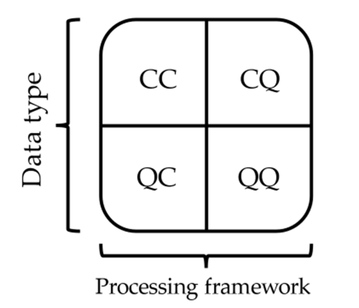
The integration between classical ML and the newer quantum computer framework can be achieved in diverse ways, as initially proposed by Aimeur et al. [
54], and this can be visualized in
Figure 1 [
3].
From
Figure 1, we observe that the four combinations are based on the origin of the data (classical “C” or quantum “Q”) and its processing methodology (also classical or quantum). The top-left represents the classical machine learning approach, where a classical computer evaluates classical information. On the bottom-right of the chart, the quantum data being processed by a quantum machine. In the context of this project, the “CQ” approach was adopted since the Folsom dataset, which was obtained through classical means, was processed using a quantum computer.
It is important to note that a simulated quantum computer was employed for the quantum processing component of this project. The use of simulated quantum circuits is a common practice given the current state of quantum computers, which are categorized as Noisy Intermediate-Scale Quantum (NISQ) machines. Although quantum computers have advanced to the point where a significantly large number of qubits is feasible, the real quantum hardware in NISQ machines still cannot provide sufficiently long coherence times (i.e., the qubit state is not maintained long enough) and are not entirely fault-tolerant. Consequently, these devices are currently unable to deliver the theorized quantum advantage.[
55,
56,
57].
Additionally, the availability of real quantum hardware is still minimal, restricted to a few enterprises that actively invest in such technology. These limitations hamper a deeper investigation of QML methodologies, as using the real NISQ devices requires monetary investments while offering limited computational power in its current state and may require an extended queue time in order to use them [
3,
55,
56,
58,
59]. Therefore, to overcome these adversities, many researchers opt to simulate their quantum circuits, an approach adopted by the present study.
2.5.1. QNN Structure
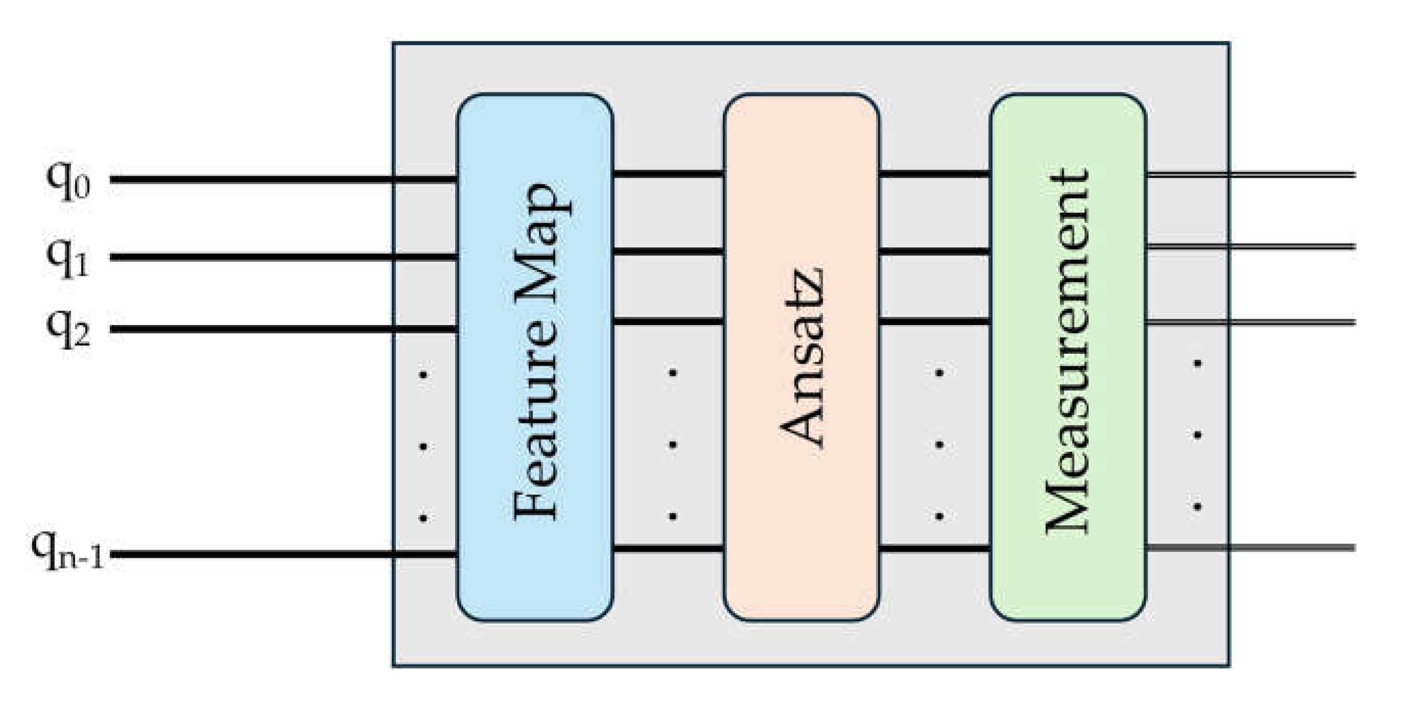
As previously mentioned, quantum computers utilize qubits to process information, a fundamental distinction between quantum and classical ML frameworks. This results in an entirely new structure for the QML approach. In the context of QML, the QNN model consists of three basic components: a Feature Map, an Ansatz, and Measurement, which are constituents of quantum circuits where data is processed. A generic QNN architecture is depicted in
Figure 2 [
60].
In
Figure 2, it is possible to visualize the structures composing the QNN model (encapsulated by the grey rectangle). The data coming from the n-qubits (
to
) enter the QNN structure from left to right, passing through the feature map, the ansatz and finally the measurement stage, where the output is mapped to a classical bit configuration.
2.5.2. Feature Map
The feature map is a fundamental component of the QNN circuit. Since the Folsom dataset is of classical origin, it must be encoded in a way that allows it to be processed by a quantum framework. The feature map serves this purpose by mapping the classical inputs into a quantum space defined within a highly complex Hilbert space, enabling a quantum computer to process the data [
61,
62,
63]. This step is arguably the most critical part of QML design, as it transforms the data structure deeply and non-linearly, achieving alterations that are not feasible through classical methods.
The current literature registers two methods for transforming classical data into a quantum format. The first one is called implicit, and it is related to directly applying a quantum circuit to implement the mapping strategy, defined as [
62]:
In Equation 4, a generic feature map takes the classical data vector , where , and encodes it into a quantum framework by using a parameterized quantum circuit containing n-qubits with initial states . The second mapping strategy is called explicit and is related to using variational quantum circuits to determine the best mapping configuration. This study employs the implicit approach to facilitate the validation of proper encoding.
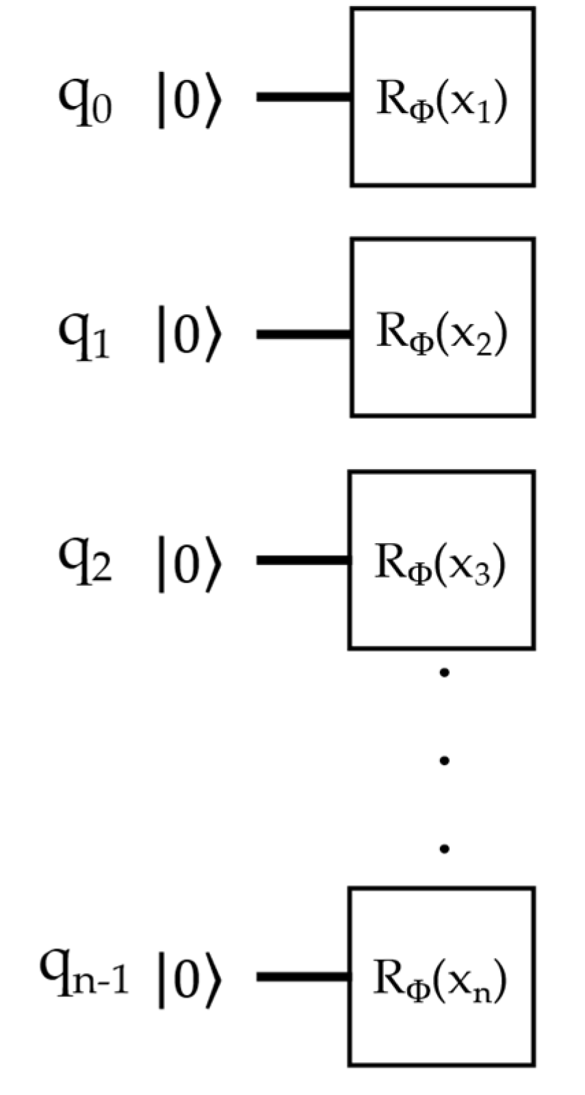
Considering the implicit feature mapping strategy, there are several distinct encoding strategies that can be applied. In the context of this project, two feature mapping approaches were investigated. The first one is called angle encoding. This approach is very simple, consisting of applying rotational quantum gates to all n-qubits in the quantum circuit. However, it still offers a powerful way to transform classical data into a quantum paradigm [
3,
52]. Each rotational gate is parameterized, taking as input the numerical input vector
from the classical dataset. Later, the input information is passed as the rotation angles for the quantum gates [
52]. Therefore, the angle encoding uses the number of quantum qubits in its circuit with the same dimensions in the dataset, i.e., the total of predictors used to forecast solar irradiation [
64]. The angle encoding mapping strategy can be represented mathematically by the following equation:
Equation 5 informs that, for a n-qubit system, the rotational gate
is applied to each one of the input parameters of the original classical dataset, resulting in the quantum state
.
Figure 3 represents a generic angle encoding mapping for n-qubits at an initial
state.
In this approach,
can assume any Pauli’s gate form, i.e., X, Y, Z or I. Detailed information regarding these quantum gates can be found in dedicated references such as in Nielsen and Chuang [
51].
The second feature mapping strategy investigated in this project was the ZZ feature map. It is the second-order Pauli expansion circuit [
58]. This approach maps classical data to a quantum framework using a quantum circuit that transforms input data as [
65]:
In Equation 6, the mapping quantum circuit
results from a relationship between the data-mapping term
and the Pauli gates,
, having a diagonal form [
66]. Furthermore, S represents a set of qubit indices in the feature map; and I is a set containing all these index sets. Commonly, the term
is defined as:
The ZZ feature map is also a parameterized circuit, where the input values from its gates come from the classical dataset. The ZZ feature map circuit is presented in
Figure 4 [
52].
From
Figure 4, the ZZ feature map initiates its circuit by applying Hadamard gates to the initial
state of the n-qubit system. It then proceeds to apply a rotation, where
. After that, the circuit utilizes controlled-NOT gates pairwise, i.e., it takes {j, k} ⊆ {q
0, q
1, …, q
n-1} for j < k, to implement entangle states in the system [
52].
2.5.3. Ansatz
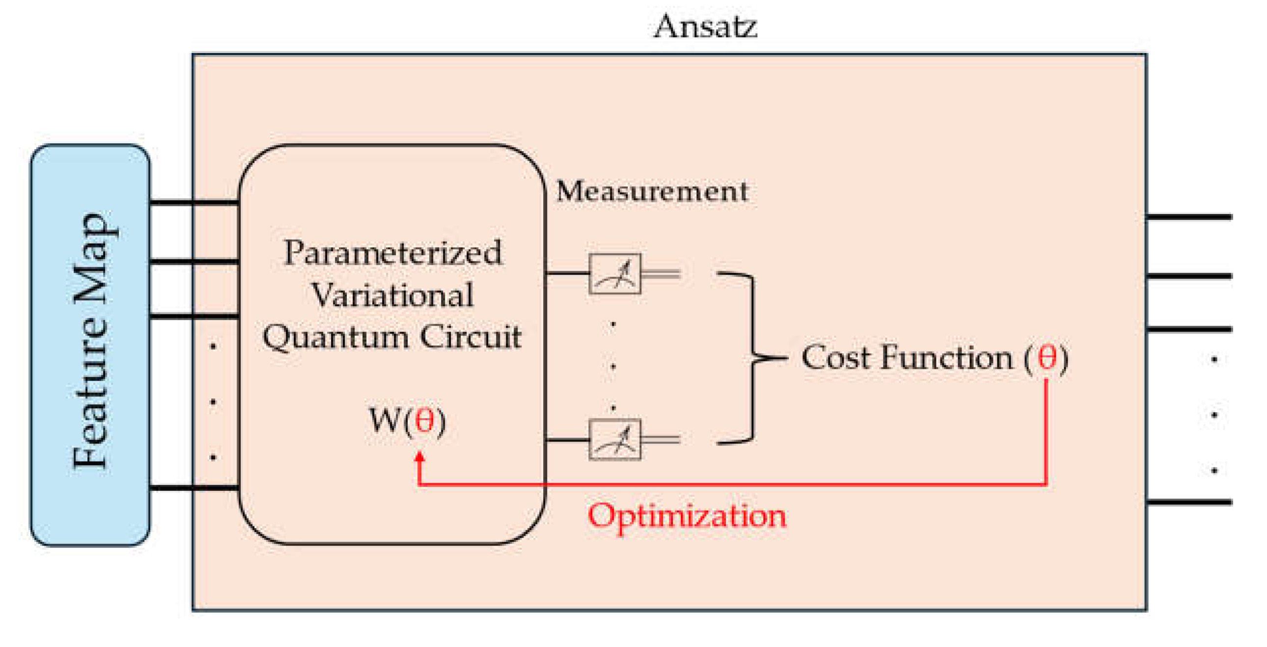
The second component of the QNN structure is the ansatz. In quantum computing, ansatz refers to the initial guess for a quantum state, which will be used as a starting point for the computation. In the context of the QNN model, similarly to classical ML, it assumes the role of the training weights of the QML. To this end, the ansatz is implemented as a parameterized variational quantum circuit. The ansatz has parameters trained for each iteration through a classical optimization algorithm, reckoned by a classical computer [
67]. A generic variational quantum circuit configuration is depicted as follows [
3].
From
Figure 5, the quantum circuit's parameters, the ansatz takes as input the previously mapped classical data. Then, its parameters θ are updated each iteration after consulting the cost function value. This process is usually done by an iterative classical optimization algorithm, which aims to reduce its value each iteration. Note that, at this point, the measurement shown in
Figure 5 refers to the ansatz’s optimization process not the final measurement performed at the end of the QNN structure (
Figure 2).
For this project, three different ansazts were investigated. The first is a simple Ry ansatz, similar to the parameterized quantum circuit previously discussed for the feature map. It consists of applying parameterized Pauli Y quantum gates. The second strategy was the Two Local ansatz. This ansatz is composed of alternating rotations and entanglement layers using parameterized gates [
68,
69]. The rotational gates are applied individually for each qubit, while the entanglement is issued over two qubits according to the desired entanglement strategy. Two entanglement strategies were evaluated in this project: linear and full entanglement. The former consists of entangling a i-th qubit with its successor i+1 for all qubits where
for a n-qubit system. The latter entanglement strategy consists of entangling all qubits with each other. The qubit entanglement may be repeated. An example for the TwoLocal quantum circuit ansatz with linear entanglement and two repetitions is depicted as follows [
70].
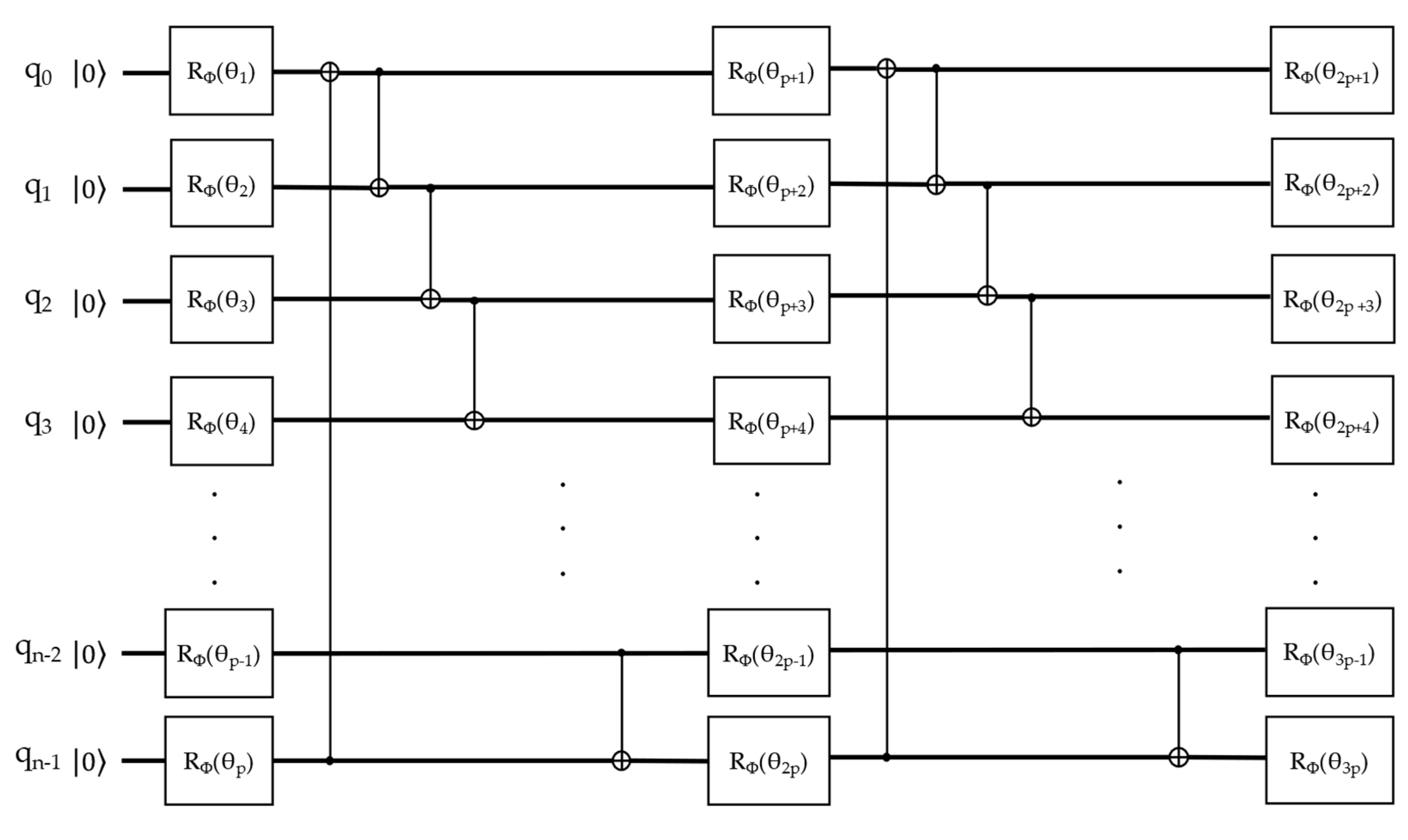
Figure 6 depicts a TwoLocal Ansatz with linear entanglement and two repetitions. It is possible to visualize that the rotational gates
accept parameterized values θ as inputs. These values represent the total change in qubit orientation, measured in radians. The total of parameters to be trained will depend on the total number of repetitions in the ansatz circuit. In the given example, since the quantity of qubits is the same as the number of dimensions in the classical dataset, defined as
, there is a total of p parameters in the first rotational layer (i.e., p = n-1). Afterwards, linear entanglement is implemented using controlled-NOT gates in pairwise fashion. Later, the first repetition takes place, doubling the total count of parameters that can be trained. This is followed by another linear entanglement, which precedes the second repetition. In this example, a total of 3p trainable weights need to be determined by the optimization algorithm.
The final ansatz used in this project was the Quantum Approximate optimization Algorithm (QAOA). It is a hybrid ansatz approach combining classical and quantum frameworks [
71]. The QAOA is a more specific form of variational quantum eigensolvers (VQE) quantum circuits, which aim to find the lowest eigenvalue of the Hamiltonian of a system [
52,
72]. To this end, the parameterized ansatz circuit prepares the quantum state such as
, where
represents the parameterized ansatz. In this context, this relationship can be rewritten as [
3]:
In Equation 8, the cost function,
, is calculated using the expected values of the system's Hamiltonians. The cost function is then minimized using classical optimizers algorithms [
3,
73]. Differently from the VQE, the QAOA approach uses a specially optimized ansatz, consisting of unique parameterizations of the problem Hamiltonian and rotational gates. The main configuration of QAOA is determined by a single integer parameter, which sets the depth of the ansatz circuit and directly influences the quality of the approximated result [
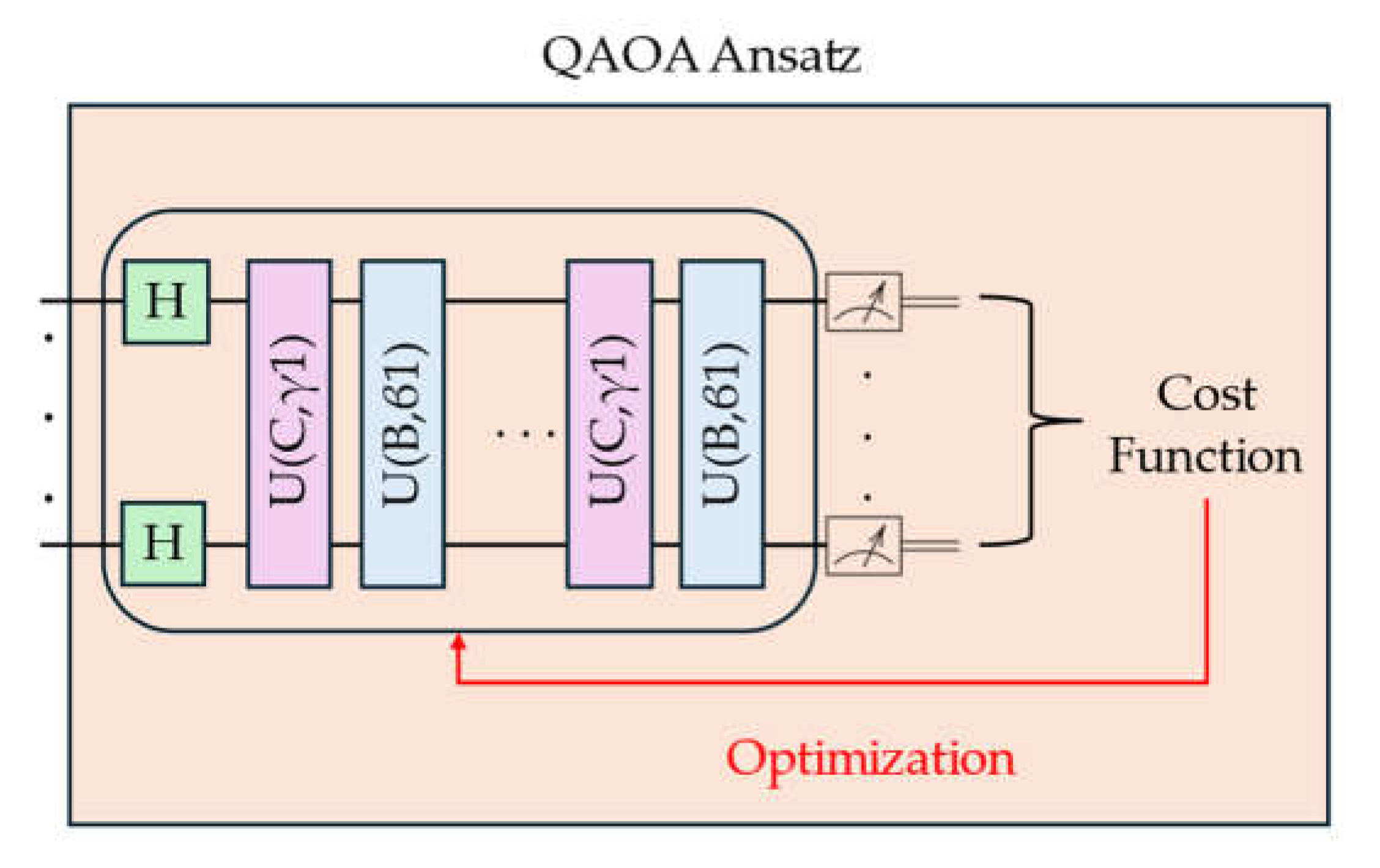
71]. A generic quantum circuit representing the QAOA ansatz is presented as follows [
3].
In
Figure 7,
C and
B define the ansatz state starting with a uniform superposition, after implementing the Hadamard gates upon all the qubits. The term
C is defined as
, where
represents a string satisfying a set of
, and the diagonal element of the Hamiltonian of a system,
, is defined as
= C(z). The term B represents the sum of Pauli X operators in the quantum circuit
. Finally,
and
[
3].
Beyond the number of qubits and the quantum gates composing them, the number of circuit repetitions also significantly characterizes both feature maps and ansatz. This is repeating the circuit in sequence m-times to the same qubits [
3]. This results in an embedded circuit in the form
. Considering the ansatz structure, repetition of its quantum circuit can be can be compared to classical layers in a classical neural network [
74]. Works on this subject have shown that repeating circuits for feature maps can encode data to come up with universal approximation theorems of QML algorithms when
, improving their output [
3]. In this project, a repetition of 1 and 2 were investigated when using the TwoLocal ansatz, as previously discussed.
2.5.4. Optimization Algorithm
Optimization algorithms play an essential role in both classical and quantum ML models. There are several strategies to optimize the cost function. In this project three optimization algorithms were investigated.
The first one is the Constrained Optimization BY Linear Approximation (COBYLA) algorithm. It is a method of numerical optimization used for problems with constraints, where the derivative of the objective function is not known. [
75]. It minimizes a scalar function of one or more variables using linear approximation over a simplex, not requiring the cost function gradient to converge, thus mitigating errors related to gradient evaluation [
76,
77,
78]. Its usage in QML models has been investigated in previous studies, showing to require a reduced number of iterations and provides good accuracy [
78,
79].
The second optimizer investigated was the Limited-memory Broyden-Fletcher-Goldfarb-Shanno Bound (L-BFGS-B). This is a quasi-Newton algorithm, meaning it does not require a second derivative of the objective function to minimize the value of a differentiable scalar function. The L-BFGS-B is an interactive model that solves unconstrained, non-linear optimization problems, updating the estimated value of the objective function with each iteration. [
80,
81]. Application of this optimization strategy for quantum problems can be found in the literature, achieving good convergence speed and accuracy [
82,
83].
Finally, the last approach investigated in this project was the Quantum Natural Simultaneous Perturbation Stochastic Approximation (QN-SPSA) optimizer. Different from the previous optimizers, this algorithm is a gradient-based approach to minimize the cost function value. This is done by taking the derivative of an objective function, f(x), and changing the x-value to minimize it for each step. Considering the case for multiple inputs, f(x
1, ... x
n), the optimization must consider the partial derivatives of the function concerning each one of its inputs. In this case, one must calculate the gradient of the function
. Thus, for the latter case, the new values x that minimize f(x) for an arbitrary time-step can be calculated as [
40,
42]:
where in Equation 8, the updated values of the attribute
result from the variation of the previous
by an amount
of the gradient of the function
. Here,
is the learning rate,
, and it regulates the total of the change attribute to the new vector. The learning rate, a hyperparameter of the gradient descent optimizer, has a direct influence on the convergence of the cost function. Slight values for the learning rate may require more steps, t, to achieve convergence. Conversely, larger learning rate amounts can cause the gradient change to become too unstable, even preventing the function from converging towards its minima [
40].
The QN-SPSA optimizer is based on the SPSA one [
84], but seeks to achieve convergence by sampling the natural gradient instead of the first-order one. This approach resembles the Monte Carlo method, where the higher the number of samplings, the more accurate the model is. This may lead to an exact, analytic result for the objective function [
85]. The QN-SPSA is well-suited for use in large-scale population models, adaptive modeling, and optimization of simulations. This makes the QN-SPSA approach to speed up the natural gradient calculation by decreasing in expense of its accuracy [
85].
The QN-SPSA implementation in Qiskit requires the fidelity and perturbation values when a specific learning rate number is passed to its function. The fidelity refers to the measurement of the closeness between two quantum states, which in this case are the Hessian of the fidelity matrix defined by the ansatz and its real value. The perturbation refers to the magnitude of the fluctuations on the parameters of the quantum circuit for the finite difference approximation of the gradients. Perturbation and learning rate can be set to have the same values when implementing the QN-SPSA optimizer [
84]. It achieves this by approximating Hessian of the fidelity of the ansatz circuit.
2.5.5. Measurement
The final step of the QNN structure is measuring the achieved quantum state after previous data processing by the feature map and ansatz quantum. Differently from quantum gates, which apply reversible operations, the measurement of the qubit state is not reversible. The measurement of a qubit’s state makes it collapse into one of its possible states defined in Equation 2 [
53]. As previously mentioned, the larger the amplitude value, the more probable the wave-function is to collapse into a specific quantum state.
3. Results
The classical forecasting models were implemented using the Scikit-Learn library for Python [
86], while the QNN approach was built and simulated using Qiskit [
87]. The hyperparameters of the classical ML models were selected using the GridSearch strategy, but for GMDH which is a self-organizing model. The dataset was split in the 80/20 Pareto fashion for the training and testing phases, without shuffling the dataset. The computer used to build and run the models has a 13
th generation i7 processor, 32 Gb of RAM, and an RTX 4080 GPU.
The ML and QNN models’ performances were evaluated using the root mean square error (RMSE), the coefficient of determination (R2) and the forecast skill (FS). These are some of the commonly used metrics to analyze the performance of predictive models.
3.1. Parameter Selection
For each forecasting horizon, the best parameters subset from the eighteen total was selected. To this end, the recursive feature elimination (RFE) was implemented [
41]. It consists of selecting the best features, starting with the whole set of predictors and selecting the most relevant ones according to a previously selected ML model. The present study implemented the RFE using a random forest (RF) model to select the best subset of attributes. Subsequently, after all the attributes have been used, they are given importance. Finally, the least important predictor is removed, and the RFE restarts. This process is repeated until a desired number of features is achieved.
Different features values were evaluated. It was observed that, for smaller numbers, RFE would return only attributes related to one type of data information. This is: the selected parameters would be temporal (Bi, Vi, and Li) or spatial (R, B, G, and their derivates). Finally, the total of attributes was set to 5. The motivation behind this is twofold:
- 6.
To keep both information from statistical features, related to temporal information, and sky image features, related to spatial data.
- 7.
To keep the problem complexity low for quantum machine learning simulation,
From the RFE output, it was observed that for forecasting intervals of 5 and 10 minutes, most of the predictors were tied to the dataset’s temporal dimension, encompassing elements B, V, and L, along with two spatial predictors. However, as the forecasting window expanded, the balance shifted. This time, three out of five predictors were associated with the dataset’s spatial dimension, i.e., sky images, leaving only two tied to the temporal aspect. This suggests a dynamic interaction between spatial and temporal factors depending on the length of the forecasting horizon, where spatial information conveys more relevant information for solar irradiance forecasting. The selected predictors are presented in the following
Table 2:
3.2. Feature Map Quantum Circuit Configuration Selection
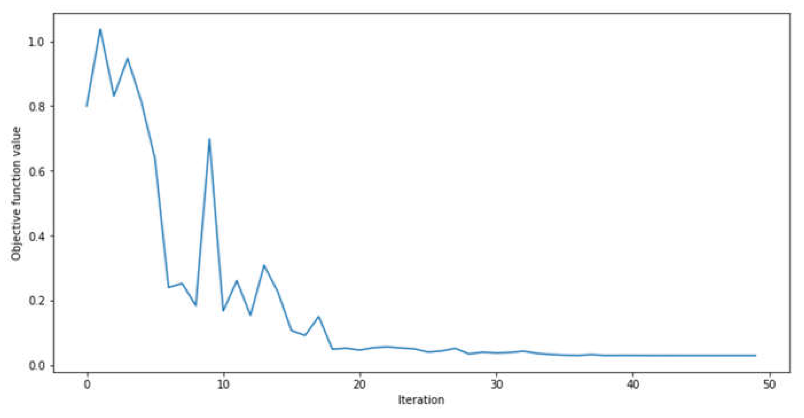
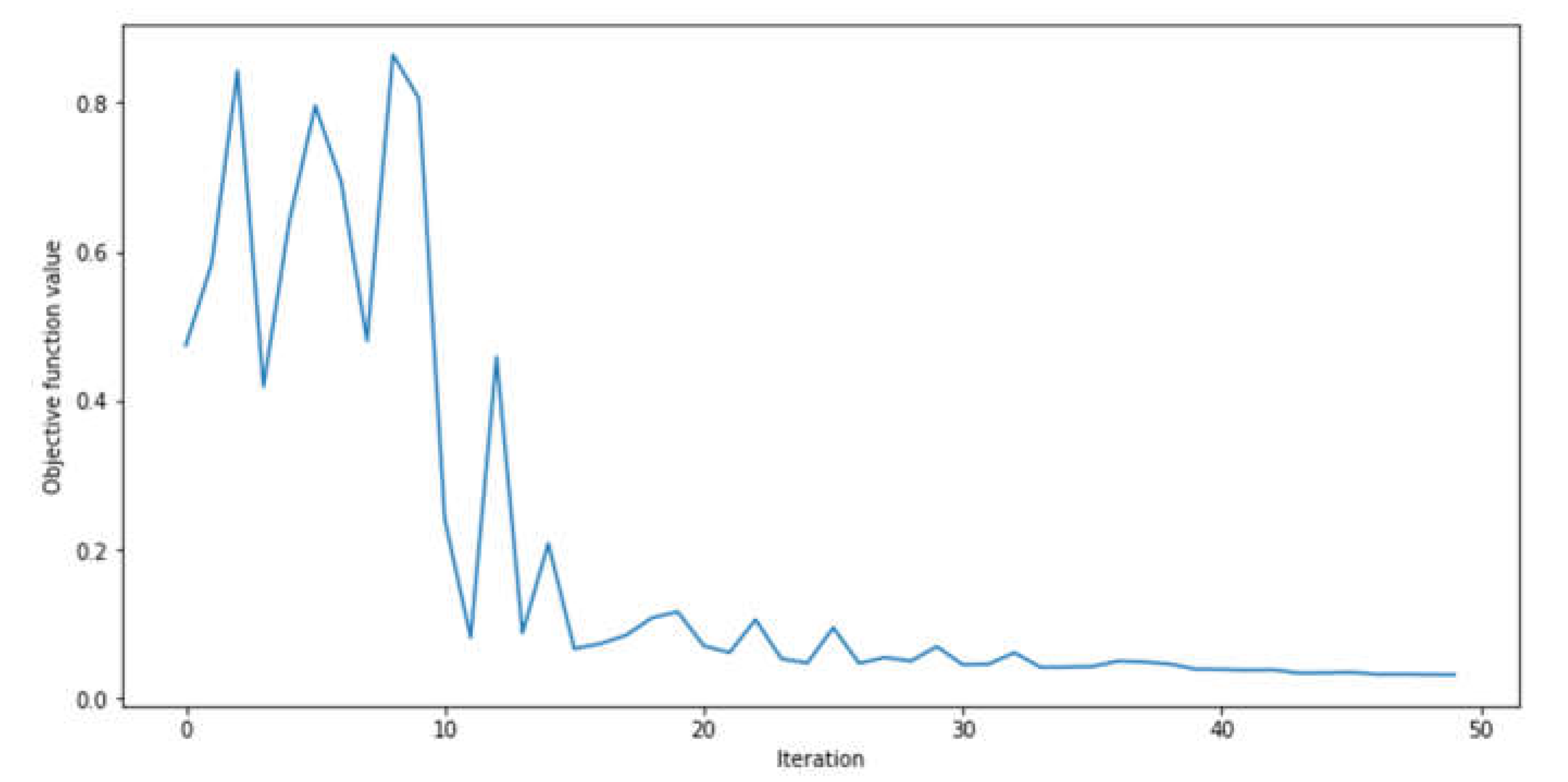
For the feature map quantum circuit, different rotations were assessed for the angle encoding strategy. The 5 minutes prediction window and global horizontal irradiance were used to benchmark the best feature map strategy. During this phase, we kept the ansatz constant, applying a simple rotational Pauli Y gate to each qubit in the circuit. We also used the COBYLA algorithm for optimization. It’s worth noting that we did test different ansatz rotations and optimization algorithms during this phase. However, these alternatives did not yield better results than the chosen configuration. Due to its significant computational time requirements, the TwoLocal ansatz was not considered during this phase. The Pauli Y rotation yielded an RMSE of 56.91 W/m2 and R2 of 95.99% for the selected feature map circuit configuration. At this point, Pauli X and Pauli Z gates were discarded as angle encoding strategies for the feature map quantum circuit. The graph showing the convergence of this approach is presented in the following figure:
Figure 8 shows that the feature map for the given configuration presented downward fashion from iteration one until around iteration twenty. Afterward, the results showed convergence towards.
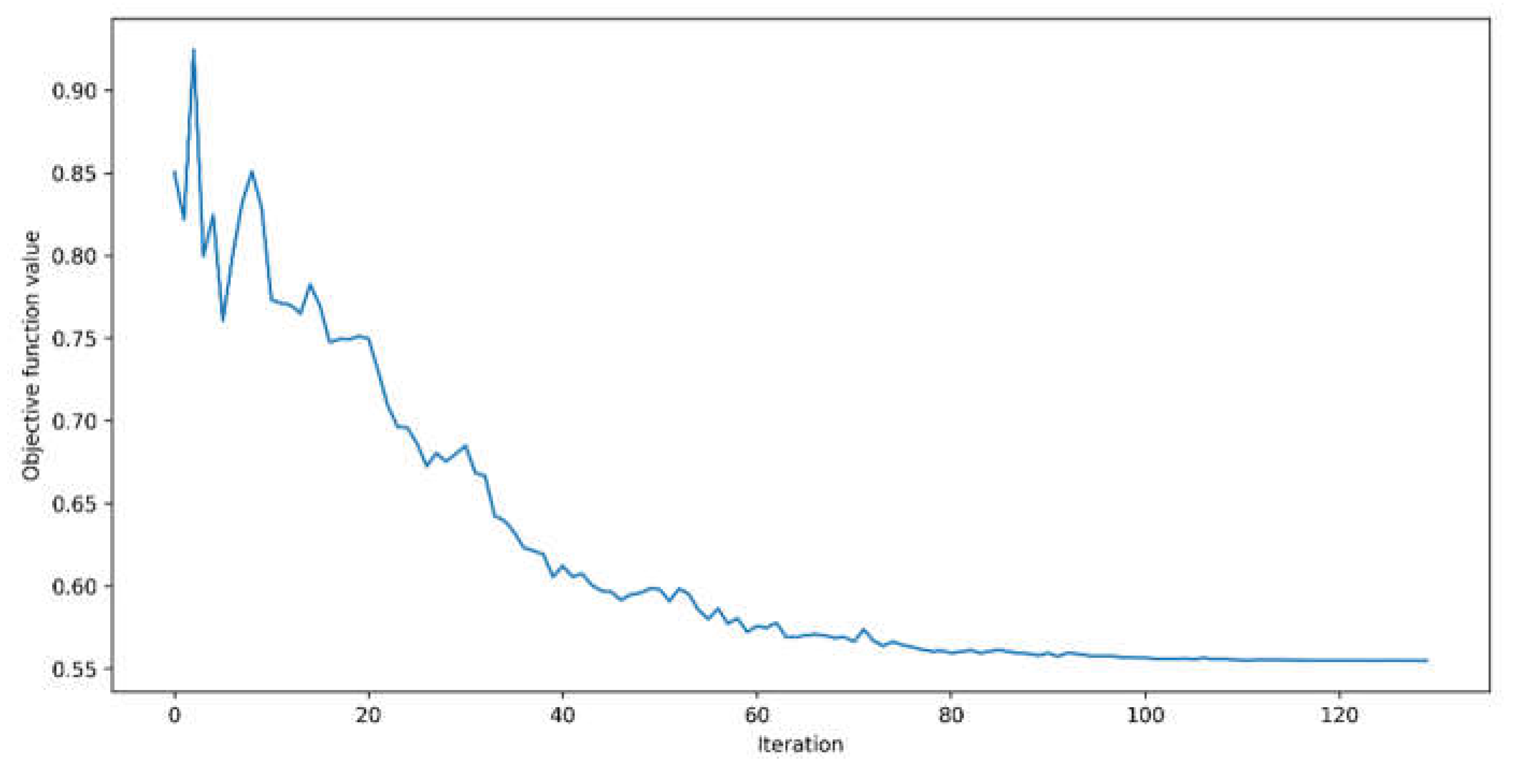
Figure 8 and
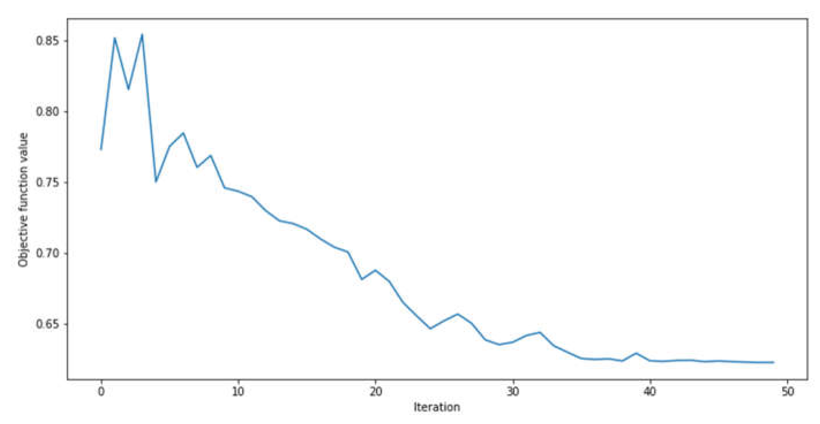
Figure 9 show that the objective function achieved convergence at around forty iterations in both cases. However, when Pauli Y was implemented as a feature map quantum circuit, the model's convergence was near zero. At the same time, in the ZZ approach, it occurred not long past the 0.65 value, indicating poorer performance than its predecessor. This can be observed by analyzing their metrics’ values, where the first approach had an RMSE of approximately 155% superior.
The second feature map investigated was the ZZ feature map. Again, using the forecasting horizon of 5 minutes for GHI as a benchmarking dataset, with Pauli Y ansatz and COBYLA optimizer, the ZZ data encoding output RMSE was 447.78 W/m2 and R2 of -1.48. The metrics elucidate that the ZZ feature map yielded inferior values than the ones provided by the Ry angle encoding. The graph showing the convergence of this approach is presented as follows:
3.3. Ansatz Quantum Circuit Configuration Selection
For the ansatz quantum circuit, it was first investigated the configuration using the previously selected Pauli Y as feature map angle encoding, with the Two Local anstaz with Pauli Y gate for rotation, controlled-x gate for entanglement, and COBYLA as optimizer for the 5 minutes forecasting horizon dataset for GHI. Note that the Pauli Y rotation used as ansatz has already been evaluated in the previous subsection (
Figure 8).
Considering the Two Local approach, two different entanglements were investigated: linear and full. The former presented better results than the latter. This configuration returned an RMSE of 58.08 W/m2 and R2 of 95.82%. The convergence for this model can be visualized in the following figure.
In
Figure 10 the convergence occurs after around 40 iterations and near to zero value for the objective function, after a bumpy behavior of its objective function value.
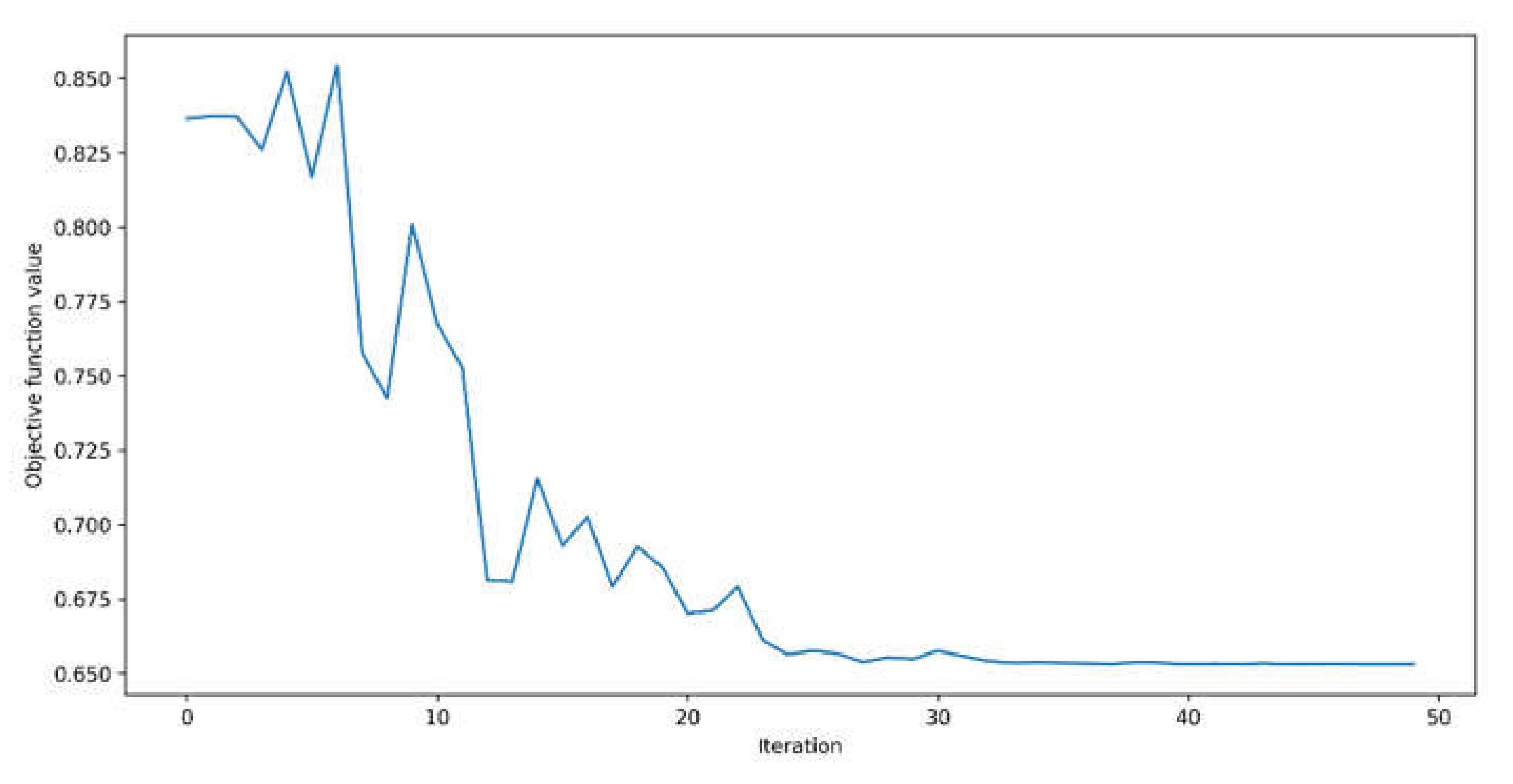
Figure 11 presents a smoother objective function value, with the convergence occurring only after 100 iterations and well before the zero value of the objective function, indicated in the image’s y-axis. The superior performance of the angle encoding approach for the feature map circuit is again observed from the given results. Considering the ZZ feature map results presented in
Figure 9 and
Figure 11, this mapping circuit was discarded as an encoding strategy for the QNN model.
Changing the rotation angle encoding to ZZ feature map and using Two Local ansatz with COBYLA optimizer, the QNN model returned subpar results, with RMSE of 402.04 W/m2 and R2 of -1.00. Its convergence can be presented in the following figure:
Finally, the QAOA was evaluated using a similar configuration, considering only the Pauli Y as a feature map quantum circuit. For this ansatz, the circuit depth was set to two. The convergence of this ansatz circuit is presented in the following figure:
Figure 12 shows that QAOA convergence is similar to the one in
Figure 10, which occurs around 30 iterations. Assessing the values present in the y-axis, the QAOA ansatz does not converge to a value near zero, indicating its suboptimal performance. The QAOA ansatz for the given configuration returned an RMSE of 498.86 W/m
2 and R
2 of -2.08, being the worst-performing approach so far.
3.4. Optimization Algorithm
The selection of the best-suited optimizer was benchmarked using the previously selected Pauli Y feature map approach for GHI forecasting 5 minutes. Pauli Y, TwoLocal, and QAOA ansatz were also evaluated during this phase. The QN-SPSA optimizer used a learning rate and perturbation values of 0.5 for the Pauli Y ansatz, 0.1 for the Two Local ansatz, and 0.3 for the QAOA ansatz. Different values were tested for QN-SPSA when applied to each ansatz were not able to surpass the results from the selected learning rates.
Table 3 compiles the results for selecting the best optimization algorithm for each evaluated configuration.
Table 3 shows that the best configuration for the QNN model is composed by the Pauli Y angle encoding as a feature map, using the Two Local ansatz, and L-BFGS-B optimizer. Regarding the QN-SPSA optimizer, it achieved better results from those output by COBYLA and L-BFGS-B when used together with Ry ansatz quantum circuit. However, when the TwoLocal approach was implemented, it was the worst-performing approach among the ones investigated. The QAOA ansatz also did not provide good outcomes for solar irradiance forecasting using the benchmarking configuration. It had a similar behavior as the one observed using the ZZ feature map, where the convergence occurred far from the zero value (
Figure 9 and
Figure 11). The following graph shows the convergence of the best-performing configuration present in the following figure:
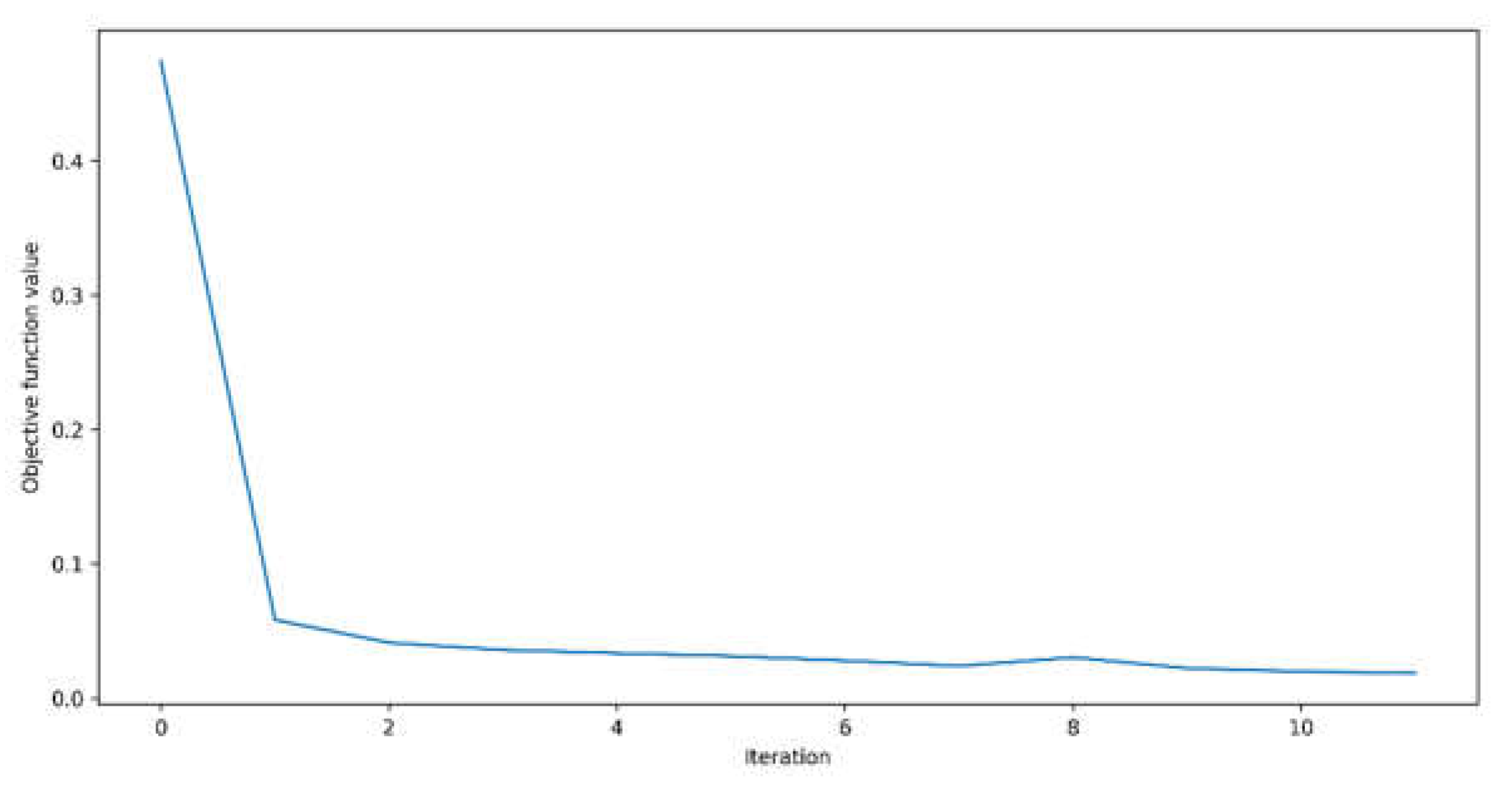
Figure 13 showcases the convergence of the best-performing configuration for QNN. Compared with
Figure 8, which uses COBYLA as an optimizer, it is noticeable that the convergence with L-BFGS-B optimizer occurs faster after around five iterations, having almost no oscillations along its path. The final configuration improved by almost 15% of the output yielded by the second-best performing configuration considering the RMSE metric (
Table 3).
3.5. Number of Repetitions for the Ansatz
Additionally, the TwoLocal ansatz was implemented using two repetitions for its configuration, already discussed in
Figure 6, using controlled-NOT gates for entanglement. To this end, the best QNN configuration, previously defined and presented in
Figure 13, was used. Using the TwoLocal ansatz with two repetitions yielded superior outputs metric values for 5-minute GHI forecasting, achieving an RMSE of 39.74 W/m
2 and R
2 of 98.04%, meaning an enhancement of over 23% compared to the second-best configuration. However, its processing time proved prohibitive, as it took eight times longer (42 hours) than the configuration presented in
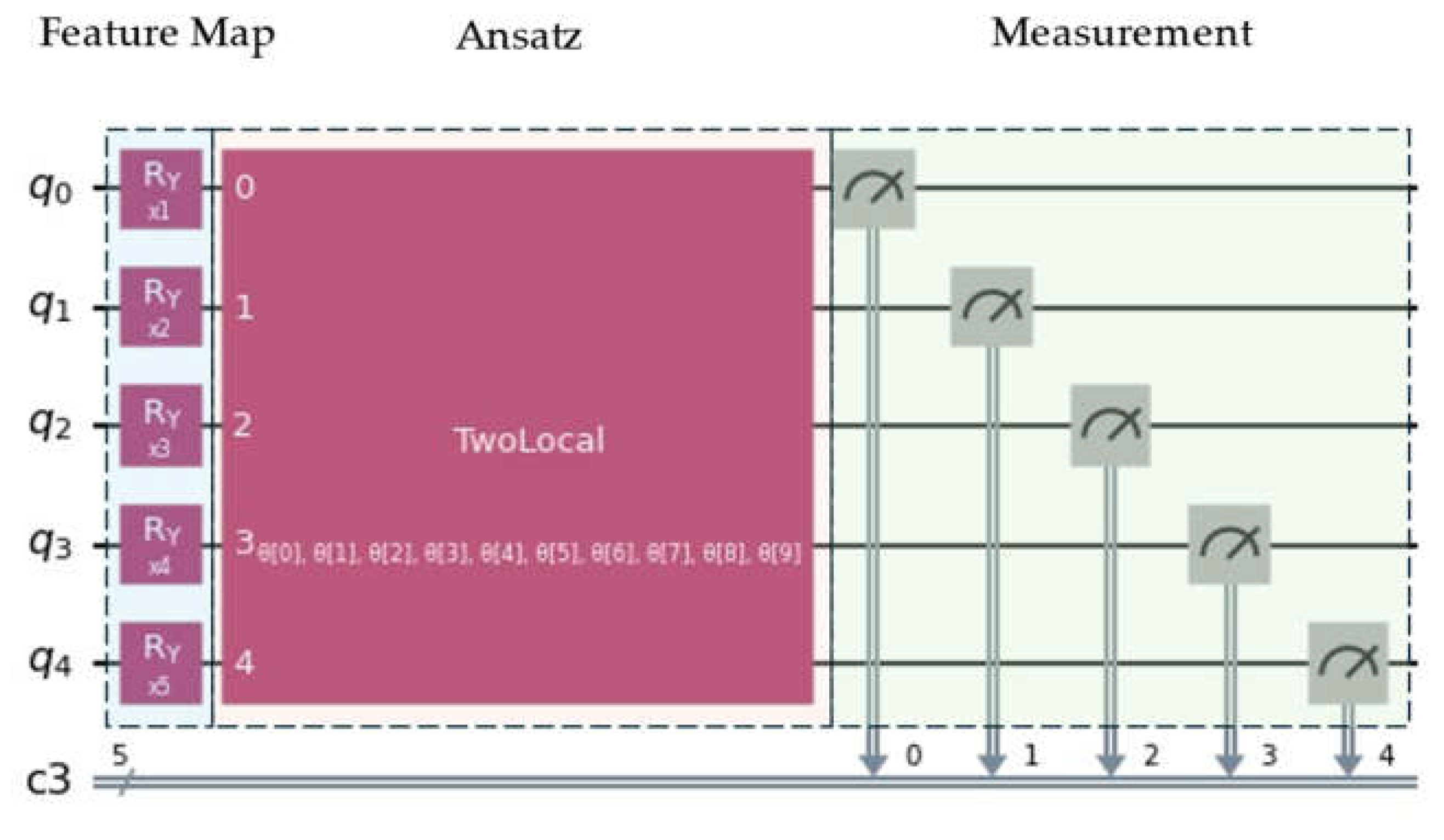
Table 3 (5 hours). Therefore, the Two Local ansatz with two repetitions was not selected for the final QNN configuration. The selected QNN configuration is presented in the following
Figure 14:
3.5. Solar Irradiance Forecasting Results
The best configurations for both classical and quantum neural networks have been selected, and the models were implemented for solar irradiance forecasting up to 3 hours ahead. Their outputs are compiled in
Table 4 and
Table 5, for GHI and DNI predictions, respectively. They are discussed in the follow-up section. The unit for RMSE metric is W/m
2.
4. Discussions
4.1. QML Models Found in the Literature
As previously stated, this study has successfully implemented a simulated QNN model utilizing the Qiskit library in Python. Existing studies have applied simulated quantum machine learning to renewable energy, whether using PennyLane [
88], Qiskit, or other available libraries.
In the work by Correa-Jullian et al. [
89], a QML model using SVM was implemented for wind turbine fault detection. Their work proved that the quantum approach could improve the results over traditional ML methodologies, being able to overcome some of them. Another quantum application in the renewable energy area can be found in the work by Sagingalieva et al. [
90]. There, the authors forecasted the photovoltaic energy output using a hybrid model, combining both classical and quantum paradigms. Their methodology achieved excellent results, proving the feasibility of this architecture in solar power prediction. The usage of QML strategies for microgrid control has been investigated in the work of Jing and colleagues [
91]. In their work, the authors used a hybrid QML model based on the Harrow Hassidim Lloyd (HHL) algorithm for microgrid management, which proved to yield remarkable results for such a task
Considering that QML is still in its nascent phase, few works addressing solar irradiance forecasting can be found. In the work by Senekane and Taele [
92], the authors implemented a quantum SVM model for solar irradiance forecasting. Their work proved the efficacy of using QML for solar irradiance forecasting. In a more recent work, the authors Sushmit and Mahbubul [
74] explored the implementation of a hybrid QML methodology for solar irradiance forecasting. Their methodology was tested across various locations and demonstrated its reliability as a forecasting tool. The structure employed in the current study mirrors the approach taken by Sushmit and Mahbubul. They utilized a parameterized quantum circuit with angle encoding as a feature map and an ansatz closely resembling the TwoLocal circuit used in this study. Their findings indicated that the QNN alone could not surpass the hybrid configurations examined, yielding RMSE and R
2 values comparable to those in
Table 4. Another study published by Yu et al. [
63] investigated the combination of a quantum circuit embedded in a recurrent neural network for GHI forecasting 1-hour. Their methodology also holds similarities to the one presented in this study, like the use of angle encoding. On the other hand, their ansatz circuit was somewhat distinct, presenting entanglement and rotation operations over the qubits. Their results for the annual prediction performance returned average results for RMSE of 61.76 W/m
2 and 94.6% for R
2, showing significant improvement over the classical ML evaluated.
The present study yields similar outcomes compared to the published studies in QML for solar irradiance forecasting. It’s noteworthy that references [
63,
74] utilize hybrid QML configurations to enhance their solar irradiance predictions [
93]. Nevertheless, based on the evaluation metrics, our study matches these predictions effectively.
4.2. GHI and DNI Forecasting Results
From tables 4 and 5, it is noticeable the superior performance of the XGBoost approach when compared to its competitors. It managed to overcome each other models for every assessed time horizon, especially for GHI, where it reached the best values of 28.74 and 98.98% for RMSE and R
2, respectively. This is not a surprise, given that the XGBoost is a well stablished ML model, and its superiority for solar energy forecasting has been attested in several studies [
25,
94,
95,
96]. The remarkable XGBoost performance can be explained twofold:
Considering the forecasting interval between 5- to 120-minutes, the models SVR and GMDH could also provide similar results to those from XGBoost, differing slightly. For this same time window, the QNN model was the fourth best-performing approach, also able to provide competitive results for GHI and DNI forecasting. The superiority of the classical models over the QNN approach is due to their much more mature implementation in a classical device, whilst QML software remains in its early stages [
99], employing very limited number of qubits. Additionally, classical ML approaches explicitly for a target task often overcome non-hybrid QML structures. Nevertheless, the quantum paradigm still can provide competitive results, as reported in [
89,
99].
Additional investigation of tables 4 and 5 reveals that for the longer forecasting horizon of 3-hours, the QNN approach managed to reach the second-best performance among the assessed models. Commonly, in time-series forecasting of spatiotemporal environmental indicators, it is expected that the predictive performance of the models decreases as the forecasting horizon expands. This behavior can be explained by the lack of additional information from the input parameters, causing the model’s performance to deteriorate for longer horizons [
21,
100]. This phenomenon occurs for the assessed models, as it is possible to observe that for the forecasting comprising the interval of 60- to 180-minutes. However, the QNN approach presents a much more robust performance than the classical ones. For instance, in the 60- to 120-minutes interval for GHI forecasting, the QNN model exhibits the less performance deterioration, as indicated by the performance metrics. This pattern does not hold for DNI forecasting, where the QNN approach displays a significantly more volatile behavior relative to other models. Remarkably, when forecasting both types of irradiances for a 3-hour period, the QNN model secured the second-best performance among the evaluated paradigms. This fact can be an indication that the quantum model may identify and retrieve relevant spatiotemporal information from the input dataset in such a manner not attainable by the current classical approaches. This capability significantly enhances its performance over extended prediction windows.
Finally, from the results in tables 4 and 5, it is also possible to observe that the overall performance for all the evaluated models decreased considerably for DNI predictions. Such a behavior is common among predictive models. The GHI represents the total radiation that arrives at the Earth’s surface from all directions. On the other hand, the DNI is a highly directional measurement, where even minor obstacles can prevent the sun-ray to reach Earth's surface, resulting in inaccuracies in its modelling [
25,
101].
Although the outcomes are suboptimal for shorter forecasting windows, i.e. from 5- to 120-minutes ahead, when compared to conventional ML frameworks, the quantum paradigm provides a compelling perspective on its utility in forecasting solar irradiance, more specifically for longer prediction intervals. This approach could potentially contribute significantly to advancing investigations in the renewable energies’ domain. As the current quantum computing technology evolves, the application of quantum circuits models using real quantum hardware is expected to become more tangible. In this context, the implementation of QML models on real quantum devices will lead to faster processing times with superior accuracy currently possible. This would ultimately allow the achievement of quantum supremacy [
5].
5. Conclusions
This study investigated the potential of applying quantum machine learning to develop a forecasting model for the GHI and DNI to optimize solar energy production. The widely recognized Folsom dataset served as the benchmark for this investigation. In this analysis, the most effective subset of predictors, encompassing both spatial and temporal attributes, were chosen for each of the forecasting horizons, which ranged from 5- to 180-minutes. The attribute selection was made using the RFE approach. Different configurations for the quantum model were examined, and the best-performing one was selected. The QML results were compared to classical ML algorithms, namely SVR, XGBoost and GMDH.
Results for the parameters selection showed that the influence of spatial-related predictors increased as the time window escalated. For the QML, the best configuration for the QNN model was achieved using Pauli Y as angle encoding for the feature map, TwoLocal ansatz with Pauli Y, and controlled-NOT gates, containing one repetition, with L-BFGS-B optimizer. The overall best results for irradiance forecasting were reached using the XGBoost model for all investigated time horizons. The QNN model, however, was able to provide competitive results for horizons spanning from 5- to 120-minutes, especially for forecasting GHI. However, the expansion of the forecasting horizon to 180-minutes revealed that the QNN model managed to overcome the classical approaches of SVR and GMDH, indicating superior capacity for identifying and extracting spatiotemporal information from the dataset than its competitors. The overall performance of the models for the DNI forecasting was inferior when compared to the GHI results.
For future works, the proposed QNN methodology could be evaluated for other renewable energy applications, such as wind speed forecasting for wind energy production. In addition, a more complex ansatz configuration containing more than one repetition could be investigated. Finally, it is expected that further investigation of the QNN model applied to real quantum hardware may allow the usage of deeper quantum circuits. This would permit the implementation of more complex quantum circuit configurations, such as larger repetitions for the ansatz, promoting a more expressive quantum machine learning model, while having improved processing time and more accurate outcomes.
Author Contributions
Conceptualization, J.V.G.T. and B.G.; methodology, P.A.C.R., J.V.G.T. and B.G.; software, V.O.S, F.P.M., P.A.C.R.; validation, P.A.C.R., J.V.G.T. and B.G.; formal analysis, P.A.C.R.; investigation, P.A.C.R., J.V.G.T. and B.G.; resources, J.V.G.T. and B.G.; data curation, J.V.G.T. and B.G.; writing—original draft preparation, V.O.S., F.P.M. and P.A.C.R.; writing—review and editing, V.O.S., F.P.M., P.A.C.R., J.V.G.T. and B.G.; visualization, V.O.S. , F.P.M. and P.A.C.R.; supervision, J.V.G.T. and B.G.; project administration, J.V.G.T. and B.G.; funding acquisition, B.G. and J.V.G.T. All authors have read and agreed to the published version of the manuscript.
Funding
This research study was funded by the Natural Sciences and Engineering Research Council of Canada (NSERC) Alliance, grant No. 401643, in association with Lakes Environmental Software Inc., and by the Conselho Nacional de Desenvolvimento Científico e Tecnológico—Brasil (CNPq), grant no. 303585/2022-6.
Data Availability Statement
Conflicts of Interest
The author Jesse Van Griensven Thé is employed by the company Lakes Environmental. The remaining authors declare that this research was conducted in the absence of any commercial or financial relationships that could be construed as potential conflicts of interest.
References
- Biamonte, J.; Wittek, P.; Pancotti, N.; Rebentrost, P.; Wiebe, N.; Lloyd, S. Quantum Machine Learning. Nature 2017, 549, 195–202. [Google Scholar] [CrossRef] [PubMed]
- Sachdeva, N.; Harnett, G.S.; Maity, S.; Marsh, S.; Wang, Y.; Winick, A.; Dougherty, R.; Canuto, D.; Chong, Y.Q.; Hush, M.; et al. Quantum Optimization Using a 127-Qubit Gate-Model IBM Quantum Computer Can Outperform Quantum Annealers for Nontrivial Binary Optimization Problems 2024.
- Schuld, M.; Petruccione, F. Machine Learning with Quantum Computers; Springer Nature, 2021; ISBN 978-3-030-83098-4.
- Cerezo, M.; Verdon, G.; Huang, H.-Y.; Cincio, L.; Coles, P.J. Challenges and Opportunities in Quantum Machine Learning. Nat Comput Sci 2022, 2, 567–576. [Google Scholar] [CrossRef] [PubMed]
- Brooks, M. THE RACE TO FIND QUANTUM COMPUTING’S SWEET SPOT. Available online: https://www.nature.com/articles/d41586-023-01692-9.pdf (accessed on 13 June 2024).
- Alchieri, L.; Badalotti, D.; Bonardi, P.; Bianco, S. An Introduction to Quantum Machine Learning: From Quantum Logic to Quantum Deep Learning. Quantum Mach. Intell. 2021, 3, 28. [Google Scholar] [CrossRef]
- Vidal Bezerra, F.D.; Pinto Marinho, F.; Costa Rocha, P.A.; Oliveira Santos, V.; Van Griensven Thé, J.; Gharabaghi, B. Machine Learning Dynamic Ensemble Methods for Solar Irradiance and Wind Speed Predictions. Atmosphere 2023, 14, 1635. [Google Scholar] [CrossRef]
- Osman, A.I.; Chen, L.; Yang, M.; Msigwa, G.; Farghali, M.; Fawzy, S.; Rooney, D.W.; Yap, P.-S. Cost, Environmental Impact, and Resilience of Renewable Energy under a Changing Climate: A Review. Environ Chem Lett 2023, 21, 741–764. [Google Scholar] [CrossRef]
- Walther, G.-R.; Post, E.; Convey, P.; Menzel, A.; Parmesan, C.; Beebee, T.J.C.; Fromentin, J.-M.; Hoegh-Guldberg, O.; Bairlein, F. Ecological Responses to Recent Climate Change. Nature 2002, 416, 389–395. [Google Scholar] [CrossRef] [PubMed]
- Duffy, P.B.; Field, C.B.; Diffenbaugh, N.S.; Doney, S.C.; Dutton, Z.; Goodman, S.; Heinzerling, L.; Hsiang, S.; Lobell, D.B.; Mickley, L.J.; et al. Strengthened Scientific Support for the Endangerment Finding for Atmospheric Greenhouse Gases. Science 2019, 363, eaat5982. [Google Scholar] [CrossRef]
- Zhang, W.; Zhou, T. Significant Increases in Extreme Precipitation and the Associations with Global Warming over the Global Land Monsoon Regions. Journal of Climate 2019, 32, 8465–8488. [Google Scholar] [CrossRef]
- Ebi, K.L.; Vanos, J.; Baldwin, J.W.; Bell, J.E.; Hondula, D.M.; Errett, N.A.; Hayes, K.; Reid, C.E.; Saha, S.; Spector, J.; et al. Extreme Weather and Climate Change: Population Health and Health System Implications. Annu. Rev. Public Health 2021, 42, 293–315. [Google Scholar] [CrossRef] [PubMed]
- Bezirtzoglou, C.; Dekas, K.; Charvalos, E. Climate Changes, Environment and Infection: Facts, Scenarios and Growing Awareness from the Public Health Community within Europe. Anaerobe 2011, 17, 337–340. [Google Scholar] [CrossRef]
- Khoury, C.K.; Brush, S.; Costich, D.E.; Curry, H.A.; Haan, S.; Engels, J.M.M.; Guarino, L.; Hoban, S.; Mercer, K.L.; Miller, A.J.; et al. Crop Genetic Erosion: Understanding and Responding to Loss of Crop Diversity. New Phytologist 2022, 233, 84–118. [Google Scholar] [CrossRef] [PubMed]
- The Economic Cost of Air Pollution: Evidence from Europe; OECD Economics Department Working Papers; 2019; Vol. 1584;
- Errigo, I.M.; Abbott, B.W.; Mendoza, D.L.; Mitchell, L.; Sayedi, S.S.; Glenn, J.; Kelly, K.E.; Beard, J.D.; Bratsman, S.; Carter, T.; et al. Human Health and Economic Costs of Air Pollution in Utah: An Expert Assessment. Atmosphere 2020, 11, 1238. [Google Scholar] [CrossRef]
- Fisher, S.; Bellinger, D.C.; Cropper, M.L.; Kumar, P.; Binagwaho, A.; Koudenoukpo, J.B.; Park, Y.; Taghian, G.; Landrigan, P.J. Air Pollution and Development in Africa: Impacts on Health, the Economy, and Human Capital. The Lancet Planetary Health 2021, 5, e681–e688. [Google Scholar] [CrossRef] [PubMed]
- Chen, Z.; Wang, F.; Liu, B.; Zhang, B. Short-Term and Long-Term Impacts of Air Pollution Control on China’s Economy. Environmental Management 2022, 70, 536–547. [Google Scholar] [CrossRef] [PubMed]
- IRENA Renewable Capacity Statistics 2024. 2024.
- World Energy Investment 2023. 2023.
- Costa Rocha, P.A.; Oliveira Santos, V.; Scott, J.; Van Griensven Thé, J.; Gharabaghi, B. Application of Graph Neural Networks to Forecast Urban Flood Events: The Case Study of the 2013 Flood of the Bow River, Calgary, Canada. International Journal of River Basin Management 2024, 1–18. [Google Scholar] [CrossRef]
- Oliveira Santos, V.; Costa Rocha, P.A.; Scott, J.; Van Griensven Thé, J.; Gharabaghi, B. Spatiotemporal Air Pollution Forecasting in Houston-TX: A Case Study for Ozone Using Deep Graph Neural Networks. Atmosphere 2023, 14, 308. [Google Scholar] [CrossRef]
- Oliveira Santos, V.; Costa Rocha, P.A.; Thé, J.V.G.; Gharabaghi, B. Graph-Based Deep Learning Model for Forecasting Chloride Concentration in Urban Streams to Protect Salt-Vulnerable Areas. Environments 2023, 10, 157. [Google Scholar] [CrossRef]
- Oliveira Santos, V.; Guimarães, B.M.D.M.; Neto, I.E.L.; de Souza Filho, F. de A.; Costa Rocha, P.A.; Thé, J.V.G.; Gharabaghi, B. Chlorophyll-a Estimation in 149 Tropical Semi-Arid Reservoirs Using Remote Sensing Data and Six Machine Learning Methods. Remote Sensing 2024, 16, 1870. [Google Scholar] [CrossRef]
- Rocha, P.A.C.; Santos, V.O. Global Horizontal and Direct Normal Solar Irradiance Modeling by the Machine Learning Methods XGBoost and Deep Neural Networks with CNN-LSTM Layers: A Case Study Using the GOES-16 Satellite Imagery. Int J Energy Environ Eng 2022, 13, 1271–1286. [Google Scholar] [CrossRef]
- Marinho, F.P.; Rocha, P.A.C.; Neto, A.R.R.; Bezerra, F.D.V. Short-Term Solar Irradiance Forecasting Using CNN-1D, LSTM, and CNN-LSTM Deep Neural Networks: A Case Study With the Folsom (USA) Dataset. Journal of Solar Energy Engineering 2023, 145, 041002. [Google Scholar] [CrossRef]
- Carneiro, T.C.; Rocha, P.A.C.; Carvalho, P.C.M.; Fernández-Ramírez, L.M. Ridge Regression Ensemble of Machine Learning Models Applied to Solar and Wind Forecasting in Brazil and Spain. Applied Energy 2022, 314, 118936. [Google Scholar] [CrossRef]
- Oliveira Santos, V.; Costa Rocha, P.A.; Scott, J.; Van Griensven Thé, J.; Gharabaghi, B. Spatiotemporal Analysis of Bidimensional Wind Speed Forecasting: Development and Thorough Assessment of LSTM and Ensemble Graph Neural Networks on the Dutch Database. Energy 2023, 278, 127852. [Google Scholar] [CrossRef]
- Liu, H.; Tang, W. Quantum Computing for Power Systems: Tutorial, Review, Challenges, and Prospects. Electric Power Systems Research 2023, 223, 109530. [Google Scholar] [CrossRef]
- Yousef, L.A.; Yousef, H.; Rocha-Meneses, L. Artificial Intelligence for Management of Variable Renewable Energy Systems: A Review of Current Status and Future Directions. Energies 2023, 16, 8057. [Google Scholar] [CrossRef]
- Pedro, H.T.C.; Larson, D.P.; Coimbra, C.F.M. A Comprehensive Dataset for the Accelerated Development and Benchmarking of Solar Forecasting Methods. Journal of Renewable and Sustainable Energy 2019, 11, 036102. [Google Scholar] [CrossRef]
- Duffie, J.A.; Beckman, W.A.; Blair, N. Solar Engineering of Thermal Processes, Photovoltaics and Wind; John Wiley & Sons, 2020; ISBN 978-1-119-54028-1.
- El Boujdaini, L.; Mezrhab, A.; Moussaoui, M.A. Artificial Neural Networks for Global and Direct Solar Irradiance Forecasting: A Case Study. Energy Sources, Part A: Recovery, Utilization, and Environmental Effects 2021, 1–21. [CrossRef]
- Cavaco, A.; Canhoto, P.; Collares Pereira, M. Procedures for Solar Radiation Data Gathering and Processing and Their Application to DNI Assessment in Southern Portugal. Renewable Energy 2021, 163, 2208–2219. [Google Scholar] [CrossRef]
- Gupta, R.; Yadav, A.K.; Jha, S.; Pathak, P.K. Long Term Estimation of Global Horizontal Irradiance Using Machine Learning Algorithms. Optik 2023, 283, 170873. [Google Scholar] [CrossRef]
- Larson, D.P.; Li, M.; Coimbra, C.F.M. SCOPE: Spectral Cloud Optical Property Estimation Using Real-Time GOES-R Longwave Imagery. Journal of Renewable and Sustainable Energy 2020, 12, 026501. [Google Scholar] [CrossRef]
- Garcia-Gutierrez, L.; Voyant, C.; Notton, G.; Almorox, J. Evaluation and Comparison of Spatial Clustering for Solar Irradiance Time Series. Applied Sciences 2022, 12, 8529. [Google Scholar] [CrossRef]
- Ineichen, P.; Perez, R. A New Airmass Independent Formulation for the Linke Turbidity Coefficient. Solar Energy 2002, 73, 151–157. [Google Scholar] [CrossRef]
- Lauret, P.; Alonso-Suárez, R.; Le Gal La Salle, J.; David, M. Solar Forecasts Based on the Clear Sky Index or the Clearness Index: Which Is Better? Solar 2022, 2, 432–444. [Google Scholar] [CrossRef]
- Géron, A. Hands-On Machine Learning with Scikit-Learn, Keras, and TensorFlow; O’Reilly Media, Inc., 2022; ISBN 978-1-09-812246-1.
- James, G.; Witten, D.; Hastie, T.; Tibshirani, R.; Taylor, J. An Introduction to Statistical Learning: With Applications in Python; Springer International Publishing, 2023; ISBN 978-3-031-38746-3.
- Goodfellow, I.; Bengio, Y.; Courville, A. Deep Learning; MIT Press, 2016; ISBN 978-0-262-03561-3.
- Chollet, F. Deep Learning with Python, Second Edition; Simon and Schuster, 2021; ISBN 978-1-63835-009-5.
- Tanveer, M.; Rajani, T.; Rastogi, R.; Shao, Y.H.; Ganaie, M.A. Comprehensive Review on Twin Support Vector Machines. Ann Oper Res 2022. [Google Scholar] [CrossRef]
- Azimi, H.; Bonakdari, H.; Ebtehaj, I.; Gharabaghi, B.; Khoshbin, F. Evolutionary Design of Generalized Group Method of Data Handling-Type Neural Network for Estimating the Hydraulic Jump Roller Length. Acta Mech 2018, 229, 1197–1214. [Google Scholar] [CrossRef]
- Elkurdy, M.; Binns, A.D.; Bonakdari, H.; Gharabaghi, B.; McBean, E. Early Detection of Riverine Flooding Events Using the Group Method of Data Handling for the Bow River, Alberta, Canada. International Journal of River Basin Management 2022, 20, 533–544. [Google Scholar] [CrossRef]
- Zaji, A.H.; Bonakdari, H.; Gharabaghi, B. Reservoir Water Level Forecasting Using Group Method of Data Handling. Acta Geophys. 2018, 66, 717–730. [Google Scholar] [CrossRef]
- Stajkowski, S.; Hotson, E.; Zorica, M.; Farghaly, H.; Bonakdari, H.; McBean, E.; Gharabaghi, B. Modeling Stormwater Management Pond Thermal Impacts during Storm Events. Journal of Hydrology 2023, 620, 129413. [Google Scholar] [CrossRef]
- Bonakdari, H.; Ebtehaj, I.; Gharabaghi, B.; Vafaeifard, M.; Akhbari, A. Calculating the Energy Consumption of Electrocoagulation Using a Generalized Structure Group Method of Data Handling Integrated with a Genetic Algorithm and Singular Value Decomposition. Clean Techn Environ Policy 2019, 21, 379–393. [Google Scholar] [CrossRef]
- Chen, T.; Guestrin, C. XGBoost: A Scalable Tree Boosting System. In Proceedings of the Proceedings of the 22nd ACM SIGKDD International Conference on Knowledge Discovery and Data Mining; ACM: San Francisco California USA, August 13, 2016; pp. 785–794. [Google Scholar]
- Nielsen, M.A.; Chuang, I.L. Quantum Computation and Quantum Information; 10th, anniversary (Eds.) ; Cambridge University Press: Cambridge ; New York, 2010; ISBN 978-1-107-00217-3.
- Combarro, E.F.; Gonzalez-Castillo, S.; Meglio, A.D. A Practical Guide to Quantum Machine Learning and Quantum Optimization: Hands-on Approach to Modern Quantum Algorithms; Packt Publishing Ltd, 2023; ISBN 978-1-80461-830-1.
- Sutor, R.S. Dancing with Qubits: How Quantum Computing Works and How It May Change the World; Expert insight; Packt: Birmingham Mumbai, 2019; ISBN 978-1-83882-736-6. [Google Scholar]
- Aïmeur, E.; Brassard, G.; Gambs, S. Machine Learning in a Quantum World. In Proceedings of the Advances in Artificial Intelligence; Vol. 3060; Tawfik, A.Y., Goodwin, S.D., Eds.; Springer Berlin Heidelberg: Berlin, Heidelberg, 2006; pp. 431–442. [Google Scholar]
- Lau, J.W.Z.; Lim, K.H.; Shrotriya, H.; Kwek, L.C. NISQ Computing: Where Are We and Where Do We Go? AAPPS Bull. 2022, 32, 27. [Google Scholar] [CrossRef]
- Li, G.; Ding, Y.; Xie, Y. Tackling the Qubit Mapping Problem for NISQ-Era Quantum Devices. In Proceedings of the Proceedings of the Twenty-Fourth International Conference on Architectural Support for Programming Languages and Operating Systems; ACM: Providence RI USA, April 4, 2019; pp. 1001–1014. [Google Scholar]
- Ullah, M.H.; Eskandarpour, R.; Zheng, H.; Khodaei, A. Quantum Computing for Smart Grid Applications. IET Generation Trans & Dist 2022, 16, 4239–4257. [Google Scholar] [CrossRef]
- Orazi, F.; Gasperini, S.; Lodi, S.; Sartori, C. Hybrid Quantum Technologies for Quantum Support Vector Machines. Information 2024, 15, 72. [Google Scholar] [CrossRef]
- Zheng, K.; Van Griensven, J.; Fraser, R. A Quantum Machine Learning Approach to Spatiotemporal Emission Modelling. Atmosphere 2023, 14, 944. [Google Scholar] [CrossRef]
- Quantum Neural Networks - Qiskit Machine Learning 0.7.2. Available online: https://qiskit-community.github.io/qiskit-machine-learning/tutorials/01_neural_networks.html (accessed on 10 June 2024).
- Schuld, M.; Killoran, N. Quantum Machine Learning in Feature Hilbert Spaces. Phys. Rev. Lett. 2019, 122, 040504. [Google Scholar] [CrossRef] [PubMed]
- Mengoni, R.; Di Pierro, A. Kernel Methods in Quantum Machine Learning. Quantum Mach. Intell. 2019, 1, 65–71. [Google Scholar] [CrossRef]
- Yu, Y.; Hu, G.; Liu, C.; Xiong, J.; Wu, Z. Prediction of Solar Irradiance One Hour Ahead Based on Quantum Long Short-Term Memory Network. IEEE Trans. Quantum Eng. 2023, 4, 1–15. [Google Scholar] [CrossRef]
- Sierra-Sosa, D.; Telahun, M.; Elmaghraby, A. TensorFlow Quantum: Impacts of Quantum State Preparation on Quantum Machine Learning Performance. IEEE Access 2020, 8, 215246–215255. [Google Scholar] [CrossRef]
- PauliFeatureMap. Available online: https://docs.quantum.ibm.com/api/qiskit/qiskit.circuit.library.PauliFeatureMap (accessed on 12 June 2024).
- Havlicek, V.; Córcoles, A.D.; Temme, K.; Harrow, A.W.; Kandala, A.; Chow, J.M.; Gambetta, J.M. Supervised Learning with Quantum Enhanced Feature Spaces. Nature 2019, 567, 209–212. [Google Scholar] [CrossRef]
- Variational Circuits — PennyLane. Available online: https://pennylane.ai/qml/glossary/variational_circuit/ (accessed on 3 June 2024).
- NLocal. Available online: https://docs.quantum.ibm.com/api/qiskit/qiskit.circuit.library.NLocal (accessed on 12 June 2024).
- TwoLocal. Available online: https://docs.quantum.ibm.com/api/qiskit/qiskit.circuit.library.TwoLocal (accessed on 12 June 2024).
- Funcke, L.; Hartung, T.; Heinemann, B.; Jansen, K.; Kropf, A.; Kühn, S.; Meloni, F.; Spataro, D.; Tüysüz, C.; Chinn Yap, Y. Studying Quantum Algorithms for Particle Track Reconstruction in the LUXE Experiment. J. Phys.: Conf. Ser. 2023, 2438, 012127. [Google Scholar] [CrossRef]
- Farhi, E.; Goldstone, J.; Gutmann, S. A Quantum Approximate Optimization Algorithm 2014.
- VQE. Available online: https://docs.quantum.ibm.com/api/qiskit/0.26/qiskit.algorithms.VQE (accessed on 12 June 2024).
- QAOA. Available online: https://docs.quantum.ibm.com/api/qiskit/0.26/qiskit.algorithms.QAOA (accessed on 12 June 2024).
- Sushmit, M.M.; Mahbubul, I.M. Forecasting Solar Irradiance with Hybrid Classical–Quantum Models: A Comprehensive Evaluation of Deep Learning and Quantum-Enhanced Techniques. Energy Conversion and Management 2023, 294, 117555. [Google Scholar] [CrossRef]
- COBYLA. Available online: https://docs.quantum.ibm.com/api/qiskit/0.26/qiskit.algorithms.optimizers.COBYLA (accessed on 12 June 2024).
- Quick, J.; Annoni, J.; King, R.; Dykes, K.; Fleming, P.; Ning, A. Optimization Under Uncertainty for Wake Steering Strategies. J. Phys.: Conf. Ser. 2017, 854, 012036. [Google Scholar] [CrossRef]
- Zhang, Z.; Zhang, C.; Qiao, Y.; Zhou, Y.; Wang, S. Design and Mass Optimization of Numerical Models for Composite Wind Turbine Blades. JMSE 2023, 11, 75. [Google Scholar] [CrossRef]
- Miki, T.; Tsukayama, D.; Okita, R.; Shimada, M.; Shirakashi, J. Variational Parameter Optimization of Quantum-Classical Hybrid Heuristics on Near-Term Quantum Computer. In Proceedings of the 2022 IEEE International Conference on Manipulation, Manufacturing and Measurement on the Nanoscale (3M-NANO); IEEE: Tianjin, China, August 8 2022; pp. 415–418. [Google Scholar]
- Miháliková, I.; Friák, M.; Pivoluska, M.; Plesch, M.; Saip, M.; Šob, M. Best-Practice Aspects of Quantum-Computer Calculations: A Case Study of the Hydrogen Molecule. Molecules 2022, 27, 597. [Google Scholar] [CrossRef] [PubMed]
- Dalvand, Z.; Hajarian, M. Solving Generalized Inverse Eigenvalue Problems via L-BFGS-B Method. Inverse Problems in Science and Engineering 2020, 28, 1719–1746. [Google Scholar] [CrossRef]
- L_BFGS_B. Available online: https://docs.quantum.ibm.com/api/qiskit/0.37/qiskit.algorithms.optimizers.L_BFGS_B (accessed on 12 June 2024).
- Wilson, M.; Stromswold, R.; Wudarski, F.; Hadfield, S.; Tubman, N.M.; Rieffel, E.G. Optimizing Quantum Heuristics with Meta-Learning. Quantum Mach. Intell. 2021, 3, 13. [Google Scholar] [CrossRef]
- Li, J.; Alam, M.; Saki, A.A.; Ghosh, S. Hierarchical Improvement of Quantum Approximate Optimization Algorithm for Object Detection: (Invited Paper). In Proceedings of the 2020 21st International Symposium on Quality Electronic Design (ISQED); IEEE: Santa Clara, CA, USA, March, 2020; pp. 335–340. [Google Scholar]
- Gacon, J.; Zoufal, C.; Carleo, G.; Woerner, S. Simultaneous Perturbation Stochastic Approximation of the Quantum Fisher Information. Quantum 2021, 5, 567. [Google Scholar] [CrossRef]
- QNSPSA. Available online: https://docs.quantum.ibm.com/api/qiskit/0.40/qiskit.algorithms.optimizers.QNSPSA (accessed on 12 June 2024).
- Pedregosa, F.; Varoquaux, G.; Gramfort, A.; Michel, V.; Thirion, B.; Grisel, O.; Blondel, M.; Prettenhofer, P.; Weiss, R.; Dubourg, V.; et al. Scikit-Learn: Machine Learning in Python. Journal of Machine Learning Research 2011, 12, 2825–2830. [Google Scholar]
- Javadi-Abhari, A.; Treinish, M.; Krsulich, K.; Wood, C.J.; Lishman, J.; Gacon, J.; Martiel, S.; Nation, P.D.; Bishop, L.S.; Cross, A.W.; et al. Quantum Computing with Qiskit 2024.
- Bergholm, V.; Izaac, J.; Schuld, M.; Gogolin, C.; Ahmed, S.; Ajith, V.; Alam, M.S.; Alonso-Linaje, G.; AkashNarayanan, B.; Asadi, A.; et al. PennyLane: Automatic Differentiation of Hybrid Quantum-Classical Computations 2022.
- Correa-Jullian, C.; Cofre-Martel, S.; San Martin, G.; Lopez Droguett, E.; De Novaes Pires Leite, G.; Costa, A. Exploring Quantum Machine Learning and Feature Reduction Techniques for Wind Turbine Pitch Fault Detection. Energies 2022, 15, 2792. [Google Scholar] [CrossRef]
- Sagingalieva, A.; Komornyik, S.; Senokosov, A.; Joshi, A.; Sedykh, A.; Mansell, C.; Tsurkan, O.; Pinto, K.; Pflitsch, M.; Melnikov, A. Photovoltaic Power Forecasting Using Quantum Machine Learning 2023.
- Jing, H.; Li, Y.; Brandsema, M.J.; Chen, Y.; Yue, M. HHL Algorithm with Mapping Function and Enhanced Sampling for Model Predictive Control in Microgrids. Applied Energy 2024, 361, 122878. [Google Scholar] [CrossRef]
- Senekane, M.; Taele, B.M. Prediction of Solar Irradiation Using Quantum Support Vector Machine Learning Algorithm. SGRE 2016, 07, 293–301. [Google Scholar] [CrossRef]
- Ayoade, O.; Rivas, P.; Orduz, J. Artificial Intelligence Computing at the Quantum Level. Data 2022, 7, 28. [Google Scholar] [CrossRef]
- Li, X.; Ma, L.; Chen, P.; Xu, H.; Xing, Q.; Yan, J.; Lu, S.; Fan, H.; Yang, L.; Cheng, Y. Probabilistic Solar Irradiance Forecasting Based on XGBoost. Energy Reports 2022, 8, 1087–1095. [Google Scholar] [CrossRef]
- Phan, Q.-T.; Wu, Y.-K.; Phan, Q.-D. Short-Term Solar Power Forecasting Using XGBoost with Numerical Weather Prediction. In Proceedings of the 2021 IEEE International Future Energy Electronics Conference (IFEEC); IEEE: Taipei, Taiwan, November 16, 2021; pp. 1–6. [Google Scholar]
- Didavi, A.B.K.; Agbokpanzo, R.G.; Agbomahena, M. Comparative Study of Decision Tree, Random Forest and XGBoost Performance in Forecasting the Power Output of a Photovoltaic System. In Proceedings of the 2021 4th International Conference on Bio-Engineering for Smart Technologies (BioSMART); IEEE: Paris / Créteil, France, December 8, 2021; pp. 1–5. [Google Scholar]
- Grinsztajn, L.; Oyallon, E.; Varoquaux, G. Why Do Tree-Based Models Still Outperform Deep Learning on Typical Tabular Data?
- Uddin, S.; Lu, H. Confirming the Statistically Significant Superiority of Tree-Based Machine Learning Algorithms over Their Counterparts for Tabular Data. PLoS ONE 2024, 19, e0301541. [Google Scholar] [CrossRef] [PubMed]
- Ajagekar, A.; You, F. Quantum Computing for Energy Systems Optimization: Challenges and Opportunities. Energy 2019, 179, 76–89. [Google Scholar] [CrossRef]
- Oliveira Santos, V.; Costa Rocha, P.A.; Scott, J.; Van Griensven Thé, J.; Gharabaghi, B. A New Graph-Based Deep Learning Model to Predict Flooding with Validation on a Case Study on the Humber River. Water 2023, 15, 1827. [Google Scholar] [CrossRef]
- Atmani, H.; Bouzgou, H.; Gueymard, C. Intra-Hour Forecasting of Direct Normal Solar Irradiance Using Variable Selection with Artificial Neural Networks.; October 23 2017.
Figure 1.
Different ways to combine classical and quantum computing strategies to perform quantum machine learning.
Figure 1.
Different ways to combine classical and quantum computing strategies to perform quantum machine learning.
Figure 2.
Generic QNN architecture.
Figure 2.
Generic QNN architecture.
Figure 3.
Generic angle encoding mapping approach. The rotational gate is applied to each one of the dimensions of the dataset.
Figure 3.
Generic angle encoding mapping approach. The rotational gate is applied to each one of the dimensions of the dataset.
Figure 4.
Generic ZZ feature map encoding approach.
Figure 4.
Generic ZZ feature map encoding approach.
Figure 5.
Generic parameterized variational quantum circuit for the ansatz structure.
Figure 5.
Generic parameterized variational quantum circuit for the ansatz structure.
Figure 6.
A TwoLocal Ansatz with linear entanglement and two repetitions.
Figure 6.
A TwoLocal Ansatz with linear entanglement and two repetitions.
Figure 7.
A generic QAOA ansatz quantum circuit.
Figure 7.
A generic QAOA ansatz quantum circuit.
Figure 8.
Graph showing the progress of the objective function value versus the iteration step using Pauli Y as the feature map angle encoding strategy, Pauli Y as ansatz, and COBYLA as optimizer.
Figure 8.
Graph showing the progress of the objective function value versus the iteration step using Pauli Y as the feature map angle encoding strategy, Pauli Y as ansatz, and COBYLA as optimizer.
Figure 9.
Graph showing the progress of the objective function value versus the iteration step using ZZ feature map strategy, Pauli Y as ansatz and COBYLA as optimizer.
Figure 9.
Graph showing the progress of the objective function value versus the iteration step using ZZ feature map strategy, Pauli Y as ansatz and COBYLA as optimizer.
Figure 10.
Graph showing the progress of the objective function value versus the iteration step using Pauli Y feature map strategy, Two Local as ansatz, and COBYLA as optimizer.
Figure 10.
Graph showing the progress of the objective function value versus the iteration step using Pauli Y feature map strategy, Two Local as ansatz, and COBYLA as optimizer.
Figure 11.
Graph showing the progress of the objective function value versus the iteration step using ZZ feature map strategy, TwoLocal as ansatz and COBYLA as optimizer.
Figure 11.
Graph showing the progress of the objective function value versus the iteration step using ZZ feature map strategy, TwoLocal as ansatz and COBYLA as optimizer.
Figure 12.
Graph showing the progress of the objective function value versus the iteration step using Pauli Y feature map strategy, QAOA as ansatz and COBYLA as optimizer.
Figure 12.
Graph showing the progress of the objective function value versus the iteration step using Pauli Y feature map strategy, QAOA as ansatz and COBYLA as optimizer.
Figure 13.
Graph showing the progress of the objective function value versus the iteration step using the best QNN configuration achieved.
Figure 13.
Graph showing the progress of the objective function value versus the iteration step using the best QNN configuration achieved.
Figure 14.
The quantum circuit selected for the QNN model. The feature map is composed of Pauli Y angle encoding, using TwoLocal ansatz with Pauli Y rotations, controlled-NOT gates for linear entanglement, and one repetition, with L-BFGS-B as optimizer.
Figure 14.
The quantum circuit selected for the QNN model. The feature map is composed of Pauli Y angle encoding, using TwoLocal ansatz with Pauli Y rotations, controlled-NOT gates for linear entanglement, and one repetition, with L-BFGS-B as optimizer.
Table 1.
Attributes and their symbols used in the present study.
Table 1.
Attributes and their symbols used in the present study.
| Attribute Name |
Attribute Symbol |
| Backward Average |
Bi
|
| Lagged Average |
Li
|
| Clear-sky Variability |
Vi
|
| Red Channel |
R |
| Green Channel |
G |
| Blue Channel |
B |
| Red-to-Blue Ratio |
RB |
| Normalized Red-to-Blue Ratio |
NRB |
| Average |
AVG |
| Standard Deviation |
STD |
| Entropy |
ENT |
Table 2.
Selected parameters using RFE.
Table 2.
Selected parameters using RFE.
| Selected Features |
|---|
Forecasting Horizon
(minutes) |
GHI |
DNI |
| 5 |
Bi, Vi, Li, ENT(R), ENT(RB) |
Bi, Vi, Li, ENT(G), ENT(RB) |
| 10 |
Bi, Vi, Li, ENT(G), ENT(RB) |
Bi, Vi, Li, ENT(G), ENT(RB) |
| 15 |
Bi, Vi, AVG(G), ENT(B), ENT(RB) |
Bi, Vi, ENT(R), AVG(G), ENT(RB) |
| 20 |
Bi, Vi, AVG(G), ENT(G), ENT(RB) |
Bi, Vi, ENT(R), AVG(G), ENT(RB) |
| 25 |
Bi, Vi, ENT(R), AVG(G), ENT(RB) |
Bi, Vi, ENT(R), AVG(G), ENT(RB) |
| 30 |
Bi, Vi, ENT(R), AVG(G), ENT(RB) |
Bi, Vi, ENT(R), AVG(G), ENT(RB) |
| 60 |
Bi, Vi, AVG(R), ENT(G), ENT(RB) |
Bi, Vi, AVG(G), ENT(G), ENT(RB) |
| 120 |
Bi, Vi, AVG(G), ENT(G), ENT(RB) |
Vi, ENT(R), AVG(G), AVG(B), ENT(RB) |
| 180 |
Bi, Li, AVG(G), ENT(B), ENT(RB) |
Vi, Li, AVG(R), ENT(R), ENT(RB) |
Table 3.
Results for different configurations of the QNN model using Pauli Y as feature map angle encoding and different ansatz and optimizers for 5 minutes GHI forecasting.
Table 3.
Results for different configurations of the QNN model using Pauli Y as feature map angle encoding and different ansatz and optimizers for 5 minutes GHI forecasting.
| Pauli Y Feature Map |
|---|
| Ansatz, Optimizer |
RMSE
(W/m2) |
R2
|
| Ry, COBYLA |
56.91 |
95.99% |
| Ry, L BFGS B |
56.73 |
96.01% |
| Ry, QN-SPSA |
56.55 |
96.04% |
| Two Local, COBYLA |
58.08 |
95.82% |
| Two Local, L-BFGS-B |
48.98 |
97.03% |
| Two Local, QN-SPSA |
63.90 |
94.94% |
| QAOA, COBYLA |
498.86 |
-2.08 |
| QAOA, L-BFGS-B |
498.85 |
-2.08 |
| QAOA, QN-SPSA |
501.21 |
-2.11 |
Table 4.
Results for GHI forecasting by the classical and quantum ML models for all the forecasting horizons.
Table 4.
Results for GHI forecasting by the classical and quantum ML models for all the forecasting horizons.
| GHI |
|---|
Forecasting Time
(minutes) |
Algorithm |
RMSE
(W/m2) |
R
2(%) |
Forecast Skill
(%) |
| 5 |
SVR |
35.94 |
98.40 |
92.33 |
| XGBoost |
28.74 |
98.98 |
93.87 |
| GMDH |
34.82 |
98.50 |
92.58 |
| QNN |
48.98 |
97.03 |
89.55 |
| 10 |
SVR |
43.00 |
97.71 |
90.82 |
| XGBoost |
32.20 |
98.72 |
93.13 |
| GMDH |
45.56 |
97.43 |
90.28 |
| QNN |
54.48 |
96.33 |
88.38 |
| 15 |
SVR |
50.17 |
96.90 |
89.29 |
| XGBoost |
40.68 |
97.96 |
91.31 |
| GMDH |
51.62 |
96.72 |
88.98 |
| QNN |
65.56 |
94.71 |
86.00 |
| 20 |
SVR |
52.69 |
96.60 |
88.74 |
| XGBoost |
42.69 |
97.77 |
90.88 |
| GMDH |
54.15 |
96.41 |
88.42 |
| QNN |
65.40 |
94.76 |
86.02 |
| 25 |
SVR |
55.11 |
96.30 |
88.20 |
| XGBoost |
44.23 |
97.62 |
90.53 |
| GMDH |
57.57 |
95.97 |
87.68 |
| QNN |
63.09 |
95.16 |
86.50 |
| 30 |
SVR |
57.00 |
96.08 |
87.80 |
| XGBoost |
45.70 |
97.48 |
90.20 |
| GMDH |
58.30 |
95.90 |
87.50 |
| QNN |
63.97 |
95.06 |
86.30 |
| 60 |
SVR |
55.63 |
96.32 |
88.00 |
| XGBoost |
34.76 |
98.56 |
92.50 |
| GMDH |
61.08 |
95.56 |
86.82 |
| QNN |
61.20 |
95.54 |
86.80 |
| 120 |
SVR |
69.91 |
94.99 |
84.18 |
| XGBoost |
54.67 |
96.93 |
87.63 |
| GMDH |
74.91 |
94.26 |
83.05 |
| QNN |
66.24 |
95.50 |
85.01 |
| 180 |
SVR |
81.94 |
94.00 |
79.84 |
| XGBoost |
58.93 |
96.90 |
85.50 |
| GMDH |
81.90 |
94.01 |
79.85 |
| QNN |
77.55 |
94.63 |
80.92 |
Table 5.
Results for DNI forecasting by the classical and quantum ML models for all the forecasting horizons.
Table 5.
Results for DNI forecasting by the classical and quantum ML models for all the forecasting horizons.
| DNI |
|---|
Forecasting Time
(minutes) |
Algorithm |
RMSE
(W/m2) |
R
2(%) |
Forecast Skill
(%) |
| 5 |
SVR |
80.31 |
93.33 |
87.16 |
| XGBoost |
61.96 |
96.03 |
90.09 |
| GMDH |
72.08 |
94.63 |
88.47 |
| QNN |
103.03 |
89.02 |
83.52 |
| 10 |
SVR |
95.17 |
90.70 |
84.75 |
| XGBoost |
77.08 |
93.90 |
87.65 |
| GMDH |
92.49 |
91.22 |
85.18 |
| QNN |
117.21 |
85.89 |
81.22 |
| 15 |
SVR |
105.25 |
88.77 |
83.08 |
| XGBoost |
87.76 |
92.19 |
85.90 |
| GMDH |
105.86 |
88.64 |
82.99 |
| QNN |
127.15 |
83.61 |
79.57 |
| 20 |
SVR |
112.31 |
87.43 |
81.88 |
| XGBoost |
93.69 |
91.25 |
84.89 |
| GMDH |
114.72 |
86.88 |
81.49 |
| QNN |
130.76 |
82.96 |
78.91 |
| 25 |
SVR |
117.58 |
86.49 |
80.95 |
| XGBoost |
98.19 |
90.58 |
84.09 |
| GMDH |
121.78 |
85.51 |
80.27 |
| QNN |
133.70 |
82.53 |
78.34 |
| 30 |
SVR |
122.84 |
85.54 |
80.00 |
| XGBoost |
102.33 |
89.97 |
83.34 |
| GMDH |
127.79 |
84.36 |
79.20 |
| QNN |
136.34 |
82.19 |
77.81 |
| 60 |
SVR |
123.77 |
85.69 |
79.53 |
| XGBoost |
84.33 |
93.35 |
86.05 |
| GMDH |
134.96 |
82.98 |
77.68 |
| QNN |
157.23 |
76.91 |
73.99 |
| 120 |
SVR |
172.05 |
77.31 |
69.11 |
| XGBoost |
107.24 |
91.19 |
80.74 |
| GMDH |
168.16 |
78.33 |
69.80 |
| QNN |
243.06 |
56.35 |
54.72 |
| 180 |
SVR |
192.58 |
74.81 |
61.46 |
| XGBoost |
145.54 |
85.61 |
70.87 |
| GMDH |
177.88 |
78.51 |
64.40 |
| QNN |
168.81 |
80.64 |
66.22 |
|
Disclaimer/Publisher’s Note: The statements, opinions and data contained in all publications are solely those of the individual author(s) and contributor(s) and not of MDPI and/or the editor(s). MDPI and/or the editor(s) disclaim responsibility for any injury to people or property resulting from any ideas, methods, instructions or products referred to in the content. |
© 2024 by the authors. Licensee MDPI, Basel, Switzerland. This article is an open access article distributed under the terms and conditions of the Creative Commons Attribution (CC BY) license (http://creativecommons.org/licenses/by/4.0/).
