Multilevel Quasi-Interpolation on Chebyshev Sparse Grids

Preprint

Article

Multilevel Quasi-Interpolation on Chebyshev Sparse Grids

Altmetrics

Downloads

111

Views

Comments

A peer-reviewed article of this preprint also exists.

Faisal Alsharif^*

This version is not peer-reviewed

Submitted:

29 June 2024

Posted:

02 July 2024

You are already at the latest version

Alerts

Abstract

This paper investigates the potential of utilising multilevel quasi-interpolation techniques on Chebyshev sparse grids for complex numerical computations. The paper starts by laying down the motivations for choosing Chebyshev sparse grids and quasi-interpolation methods with Gaussian kernels. It delves into the practical aspects of implementing these techniques. Various numerical experiments are performed to evaluate the efficiency and limitations of the multilevel quasi-sparse interpolation methods with dimensions two dimension and three dimension. The work ultimately aims to provide a comprehensive understanding of the computational efficiency and accuracy achievable through this approach, comparing its performance with traditional methods.

Keywords:

Subject: Computer Science and Mathematics - Computational Mathematics

1. Introduction

Traditional interpolation methods, such as grid-based or radial basis function interpolation, encounter computational difficulties when dealing with multidimensional datasets. The computational complexity of these methods grows exponentially with the number of dimensions, rendering them similarly unfeasible on reasonable timeframes. Consequently, novel approaches are necessary to address the challenge of interpolation in multidimensional spaces.

The need for innovative solutions has driven the development of novel numerical methods that are capable of efficiently handling 2D, 3D, or high-dimensional data using higher-performance computers [1,2]. As a result, researchers have been able to make significant advancements in the various scientific domains mentioned, enabling the development of innovative solutions to complex problems [3].

2. Chebyshev Sparse Grids Technique

In literature, it has been proposed a sparse grid technique to overcome the curse of dimensionality with equally spaced grids for higher dimensional domains [4]. Georgoulis et al. [4] proposed algorithm reduces the requirement of large number of data points on an equally spaced grid but keeps the simplicity of a grid structure in evaluating the interpolant. The construction of a sparse grid is defined as follows.

Define a multi-index

ℓ = (l_{1}, \dots, l_{d}) \in N^{d}

and

(i_{1}, \dots, i_{d}) \in N^{d}

as a spatial position. Define the point for that position as

x_{ℓ, i} = (x_{l_{1}, i_{1}}, \dots, x_{l_{d}, i_{d}}) w i t h x_{l_{j}, i_{j}} = 2 (i_{j} . 2^{- l_{j}} - 0.5) f o r j = 1, \dots, d .

We can now define the family of uniform grids

G_{ℓ}

as the set of points:

G_{ℓ} = {x_{ℓ, i} : i = (i_{1}, \dots, i_{d}), i_{j} = 0, 1, \dots, 2^{l_{j}}, j = 1, \dots, d} .

The number of points

N_{ℓ}

G_{ℓ}

is given by:

N_{ℓ} = \prod_{j = 1}^{d} (2^{l_{j}} + 1) .

If we have

ℓ = (n, \dots, n)

G_{ℓ}

is the uniform full grid of equally spaced points of level n with distances between the points given by

h = 2^{- n}

. The size of the grid

G ℓ

N = {(2^{n} + 1)}^{d}

. We will denote this full grid as

G_{n, d}

. Now, we consider a sparse subset of uniform full grid,

G_{n, d}

{\tilde{G}}_{n . d} = ⋃_{| ℓ | = n + (d - 1)} G_{ℓ}

(1)

with

| ℓ | = l_{1} + l_{2} + \dots + l_{d}

. We will refer

{\tilde{G}}_{n . d}

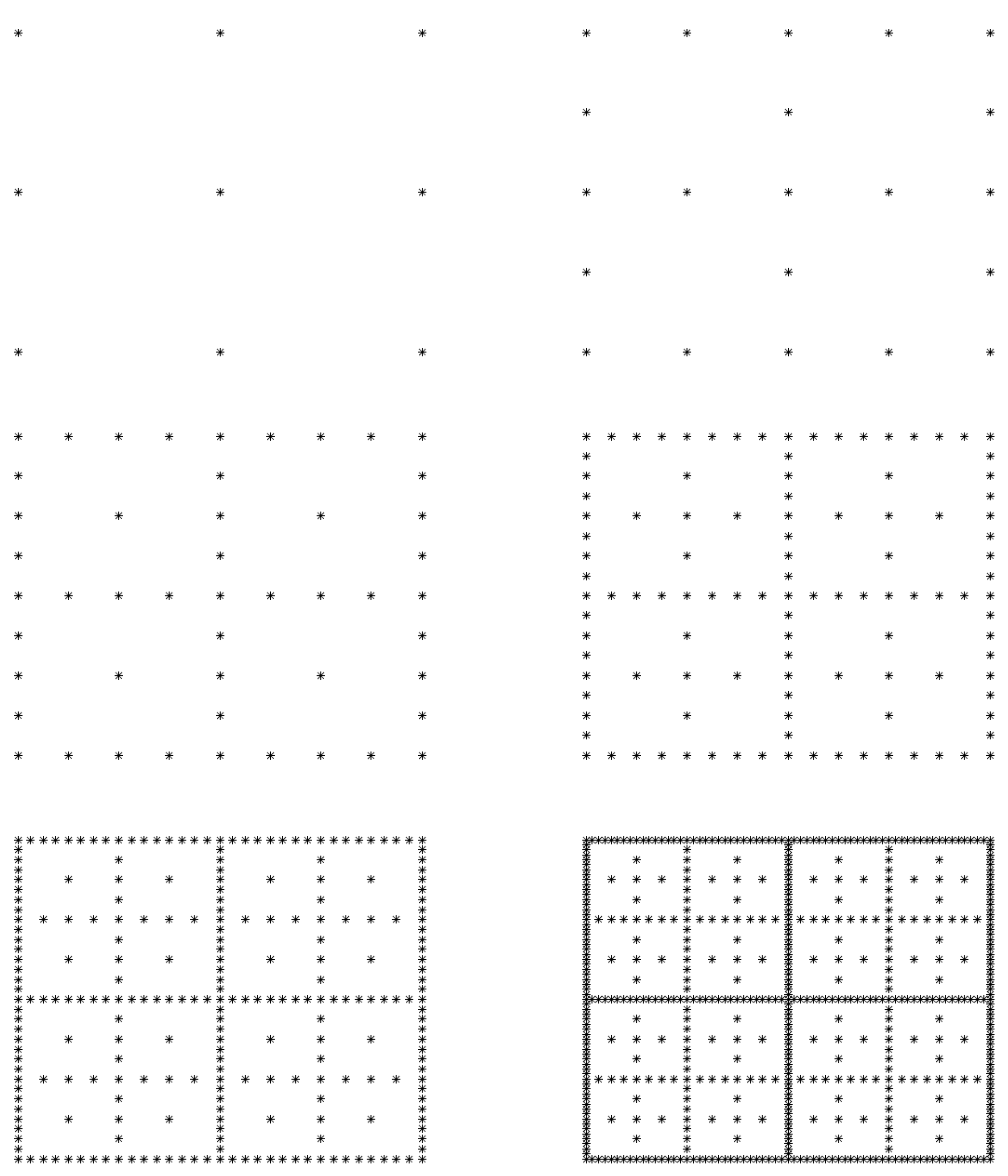
as the sparse grid of level n in dimension d. Figure 1 shows a visual representation of the sparse grid for

n = 4

and

d = 2

. Notice that some of the grid points are included in more than one sub-grid and hence there are some redundancies.

In an alternative formulation of the sparse grid, there are arguments that instead of using equally spaced grid, one can use the Chebyshev points to create the grids on

[- 1, 1]

. For the multi-index

ℓ = (l_{1}, \dots, l_{d}) \in N^{d}

and

(i_{1}, \dots, i_{d}) \in N^{d}

, we can define

x_{l_{j}, i_{j}}^{c} = - cos (\frac{2 i_{j} - 1}{2 \times 2^{l_{j}}}) f o r j = 1, \dots, d

to have the point

x_{ℓ, i}^{c} = (x_{l_{1}, i_{1}}^{c}, \dots, x_{l_{d}, i_{d}}^{c})

. Similarly, we can define the family of Chebyshev grids as:

G_{ℓ}^{c} = {x_{ℓ, i}^{c} : i = (i_{1}, \dots, i_{d}), i_{j} = 0, 1, \dots, 2^{l_{j}}, j = 1, \dots, d}

and the sparse subset of Chebyshev grids as:

{\tilde{G}}_{n . d}^{c} = ⋃_{| ℓ | = n + (d - 1)} G_{ℓ}^{c}

(2)

{\tilde{G}}_{n . d}^{c}

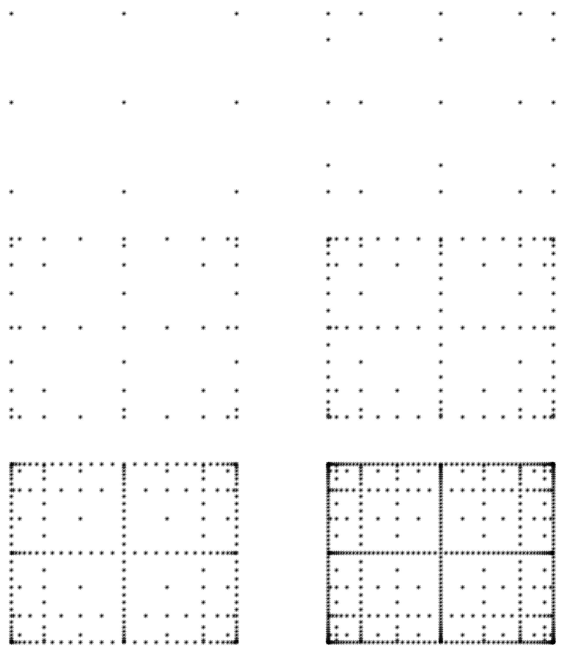
will be referred as the sparse Chebyshev grid of level n is dimension d. Figure 2 shows a visual representation of the sparse Chebyshev grid for

n = 4

and

d - 2

. We observe that the sparse grid points are not equally spaced.

3. Quasi Sparse Interpolation with Gaussian Kernels

In the previous formulation of the interpolation using RBF, we have seen that it requires to solve a system of N linear equations, where N is the total number of points. Using a sparse grid of points as defined in previous sub-section will reduce the total number of points and subsequently the total number of equations for the higher dimension compared to a full grid of points. However, that does not fully eliminate the ill-conditioning of the problems. Another method proposed in the literature to avoid solving of the system of linear equations is to use quasi-interpolation. There are extensive discussion on error estimates in quasi-interpolation in the literature ([5,6,7]).

We use the idea of quasi-interpolation on the sparse grid with anisotropic Gaussian basis functions. Let

c_{i, j} = | x_{i + 1, j} - x_{i, j} |

, the distance between the points

x_{i}

and

x_{i + 1}

in dimension j for

j = 1, \dots, d

. Then define the diagonal matrix:

A_{i} = d i a g (c_{i_{1}, 1}, \dots, c_{i_{d}, d})

where

i = (i_{1}, \dots, i_{d})

. For each multi-index ℓ, we now define anisotropic the quasi-interpolant

Q_{ℓ} f (x) = \sum_{x_{ℓ, i} \in G_{ℓ}} f (x_{ℓ, i}) ϕ_{c} (A_{i}^{- 1} (x - x_{ℓ, i})), x \in Ω .

(3)

Here we consider the Gaussian kernel

ϕ_{c} (x) = \frac{1}{\sqrt{2 π} c} exp (- \frac{x^{2}}{2 c^{2}})

with c determining the degree of smoothness of the interpolant.

To construct the quasi sparse kernel based interpolant on the sparse grid

{\tilde{G}}_{n, d}

, the anisotropic interpolants on the sub-grids

G_{ℓ}

are linear combined using the following formula:

Q_{n, d} f (x) = \sum_{j = 0}^{d - 1} {(- 1)}^{j} (\binom{d - 1}{j}) \sum_{| ℓ | = n + (d - 1) - j} Q_{ℓ} f (x) .

(4)

For example, the quasi sparse kernel based interpolation for

d = 2

would be

Q_{n, 2} f (x) = \sum_{| ℓ | = n + 1} Q_{ℓ} f (x) - \sum_{| ℓ | = n} Q_{ℓ} f (x)

and for

d = 3

, it would be

Q_{n, 3} f (x) = \sum_{| ℓ | = n + 2} Q_{ℓ} f (x) - 2 \sum_{| ℓ | = n + 1} Q_{ℓ} f (x) + \sum_{| ℓ | = n} Q_{ℓ} f (x) .

In a similar fashion, we can construct the quasi sparse kernel based interpolation formula for the sparse grids based on Chebyshev points, by replacing the grids

G_{ℓ}

G_{ℓ}^{c}

4. Multilevel Quasi Sparse Interpolation

From the construction of the sparse grids, it is obvious that the sparse grids from lower level to the upper level are nested, that is,

{\tilde{G}}_{n, d} \subset {\tilde{G}}_{n + 1, d}

for all

n \geq 1

. We have illustrated this nested nature in Figure 3 for equally spaced grid points. For Chebysheb points also, we have the nested nature of the grids and that is also shown in Figure 4. Moreover, while combining the kernel based anisotropic interpolants for each subgrid, they were appropriately scaled with the scaling being proportional to the density of the corresponding constituent subgrid. One can utilize these nested properties of the subgrids to propose a multilevel methods of interpolation with them without adding any further complexity to the quasi sparse kernel based interpolation introduced earlier. In the earlier literature ([8,9,10]), multilevel methods for radial basis functions were used to combine stationary and non-stationary interpolants to accelerate the convergence and to improve the numerical stability of the ill-conditioned problems.

The main idea of the multilevel sparse grid based quasi interpolation is to interpolate the function at the lowest level, that is, for

n = 1

and then update at each level of the sub-grids by computing the residuals at every level and then interpolating them at the higher level. More formally, we obtain the quasi sparse kernel based interpolation

Q_{n_{0}, d} f (x)

at the coarsest level 1, that is the coarsest level approximation is

S_{0, d} f (x) = Q_{n_{0}, d} u (x)

. Then we define the residual function at level j as

r_{j} (x) = f (x) - S_{j - 1, d} f (x)

and interpolate the residual function as

Δ_{j} (x) = Q_{n_{0} + j, d} r_{j} (x)

on the level

n_{0} + j

sparse grid

{\tilde{G}}_{n_{0} + j, d}

and then update the multilevel interpolant as:

S_{j, d} f (x) = S_{j - 1, d} f (x) + Δ_{j} (x), f o r 1 \leq j \leq n .

We refer to this algorithm as the multilevel quasi sparse kernel based interpolation. As the quasi sparse kernel based interpolation is being used at every level, the time-complexity of the multilevel method is linear with the levels. However, it takes more time than the usual quasi sparse interpolation for a fixed level as it evaluates the residuals at every grid point. Again, the algorithm is easily amenable for parallel computing.

5. Implementation

In this article, all algorithms and numerical experiments are implemented in Matlab 2022a. The implementation is broken down in main three parts:

Creating the sparse grids using either equally spaced grids or Chebyshev points for each level of the multilevel grid,
The anisotropic quasi-interpolation $Q_{ℓ} f (x)$ using Gaussian kernel
The algorithm for quasi-sparse interpolation, which combines the anisotropic quasi-interpolants as described earlier.

For multilevel quasi-interpolation, we implement another function to implement the algorithm.

5.1. Multilevel Quasi Sparse Interpolation

The outline for the algorithm of multilevel quasi-sparse interpolation is given in Algorithm 1. In the implementation of the multilevel quasi-sparse interpolation, after initial checks and creating sparse grid of points, if necessary, we compute the quasi-interpolation approximation using the function QSIK for the level

n = 1

. For all other levels

i > 1

, we evaluate the quasi-sparse interpolation approximation at all sparse grid points and then subtract that from the original function value to compute the residual function and then again compute the quasi-sparse approximation for the residual function at level i and added that estimate to the function approximation, we already have up to that level i. We continue computing the residual functions and updating our approximation at each level until the maximum level of evaluations n is reached. This multilevel approximation returns the function approximations at all levels

1 \leq i \leq n

. Though it requires a lot of quasi-sparse interpolation approximations at all levels, we can reduce the computation time by computing the function approximations at all levels together rather than calling the function separately for each level.

Algorithm 1: Multilevel Quasi-Sparse Interpolation Algorithm

Data: Sparse grid data decomposition

Result: The multilevel quasi-sparse interpolation

S_{n, d} f (x)

6. Numerical Experiments for Quasi-Sparse Interpolation with $d = 2$

We now illustrate the performance of the proposed quasi sparse kernel based interpolation for the following test functions:

$F_{1}^{2 d} (x, y)$ (Franke’s function)

$\begin{matrix} F_{1}^{2 d} (x, y) & = & 0.75 e^{- ({(9 x - 2)}^{2} + {(9 y - 2)}^{2}) / 4} + 0.75 e^{- {(9 x + 1)}^{2} / 49 - {(9 y + 1)}^{2} / 10} \\ + 0.5 e^{- ({(9 x - 7)}^{2} + {(9 y - 3)}^{2}) / 4} - 0.2 e^{- ({(9 x - 4)}^{2} + {(9 y - 7)}^{2})} . \end{matrix}$
$F_{2}^{2 d} (x, y) = (1 - x^{2}) (1 - y^{2})$ .
$F_{3}^{2 d} (x, y) = \sqrt{\frac{18}{π}} e^{- (x^{2} + 81 y^{2})}$ .
$F_{4}^{2 d} (x, y) = \frac{1.25 + cos (5.4 y)}{6 + 6 {(3 x - 1)}^{2}}$ .

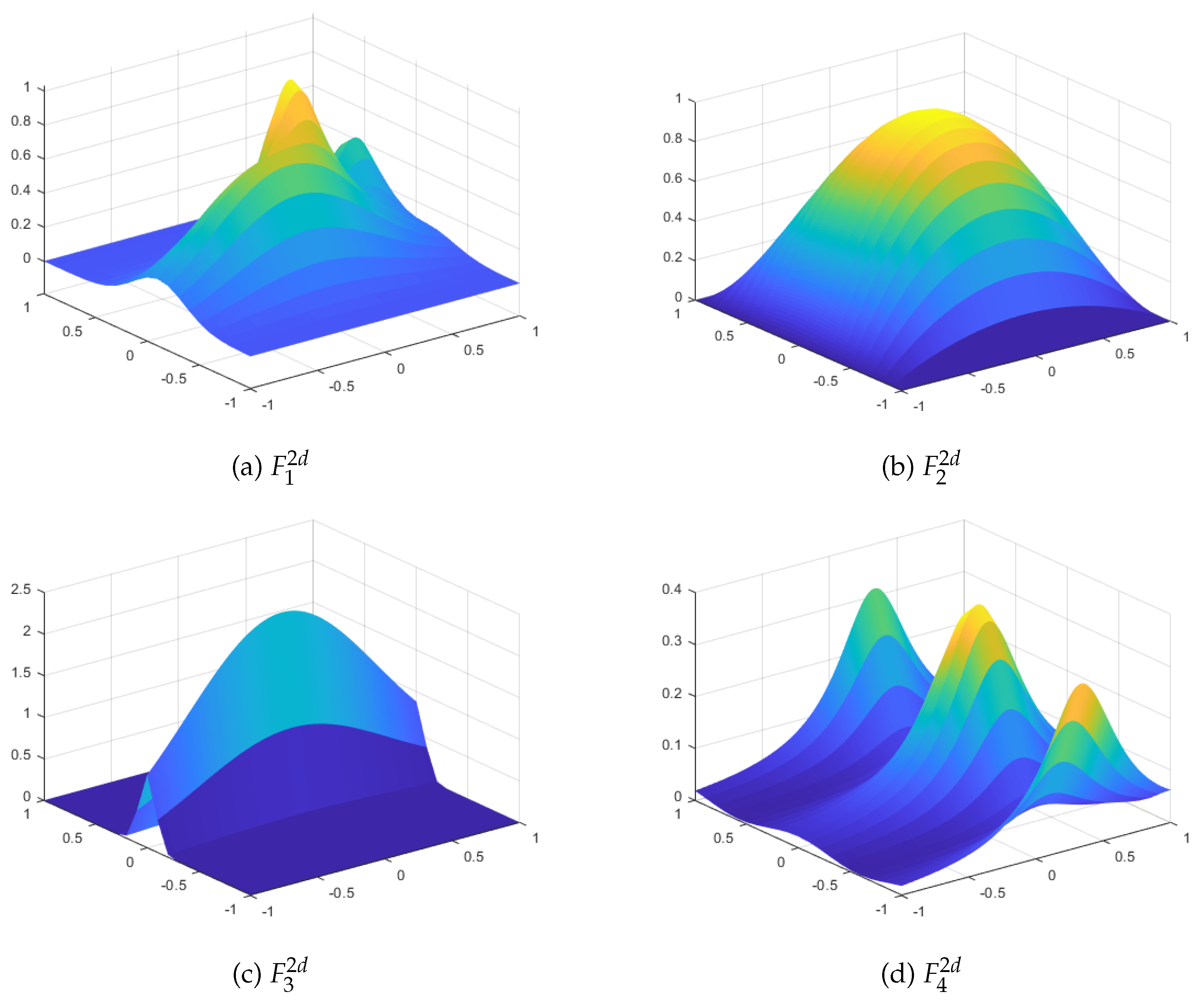
The Franke’s function is very commonly used as a test function in the interpolation literature with RBF kernels ( [11]). The others can be found in [12,13] and [14], respectively. These test functions are illustrated in Figure 5.

In all of these numerical experiments, we have used a

50 \times 50

uniform grid of points in the rectangle

[- 1, 1] \times [- 1, 1]

. The error in approximation is reported as the maximum modulus error, that is,

∥ f - Q_{n, d} f ∥

and root-mean-square error as defined below:

\sqrt{\frac{1}{N_{e}} \sum_{i = 1}^{n} {(f (x_{i}) - Q_{n, d} f (x_{i}))}^{2}}

where

x_{i}

i = 1, \dots, N_{e}

are the evaluation points and

N_{e}

is the total number of evaluation points. We also report the number of points in the sparse grid

{\tilde{G}}_{n, d}

(or

{\tilde{G}}_{n, d}^{c}

) as SGnode and the number of points actually used in the computation as some of the points are revisited in the sparse grid computations as DoF.

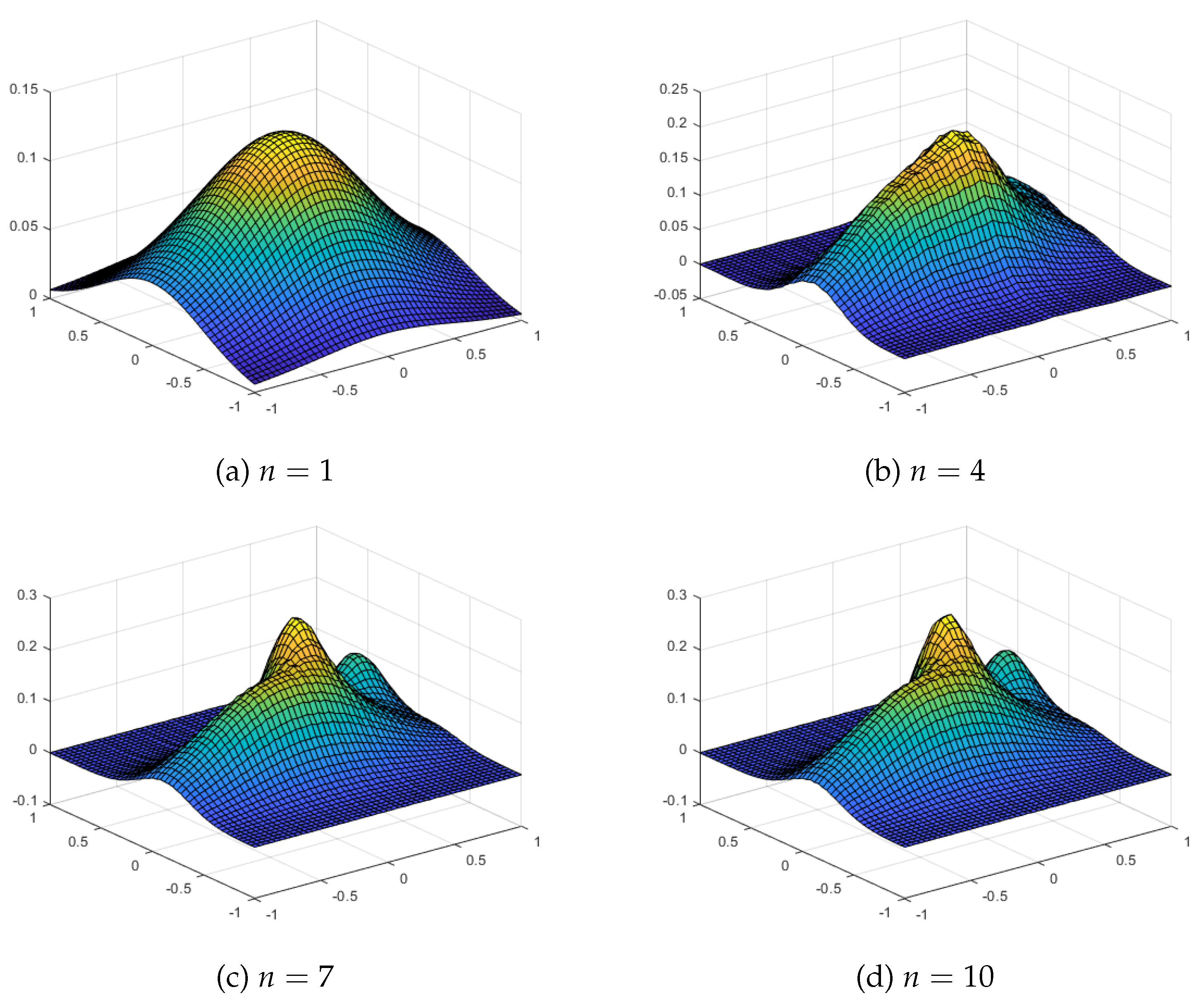
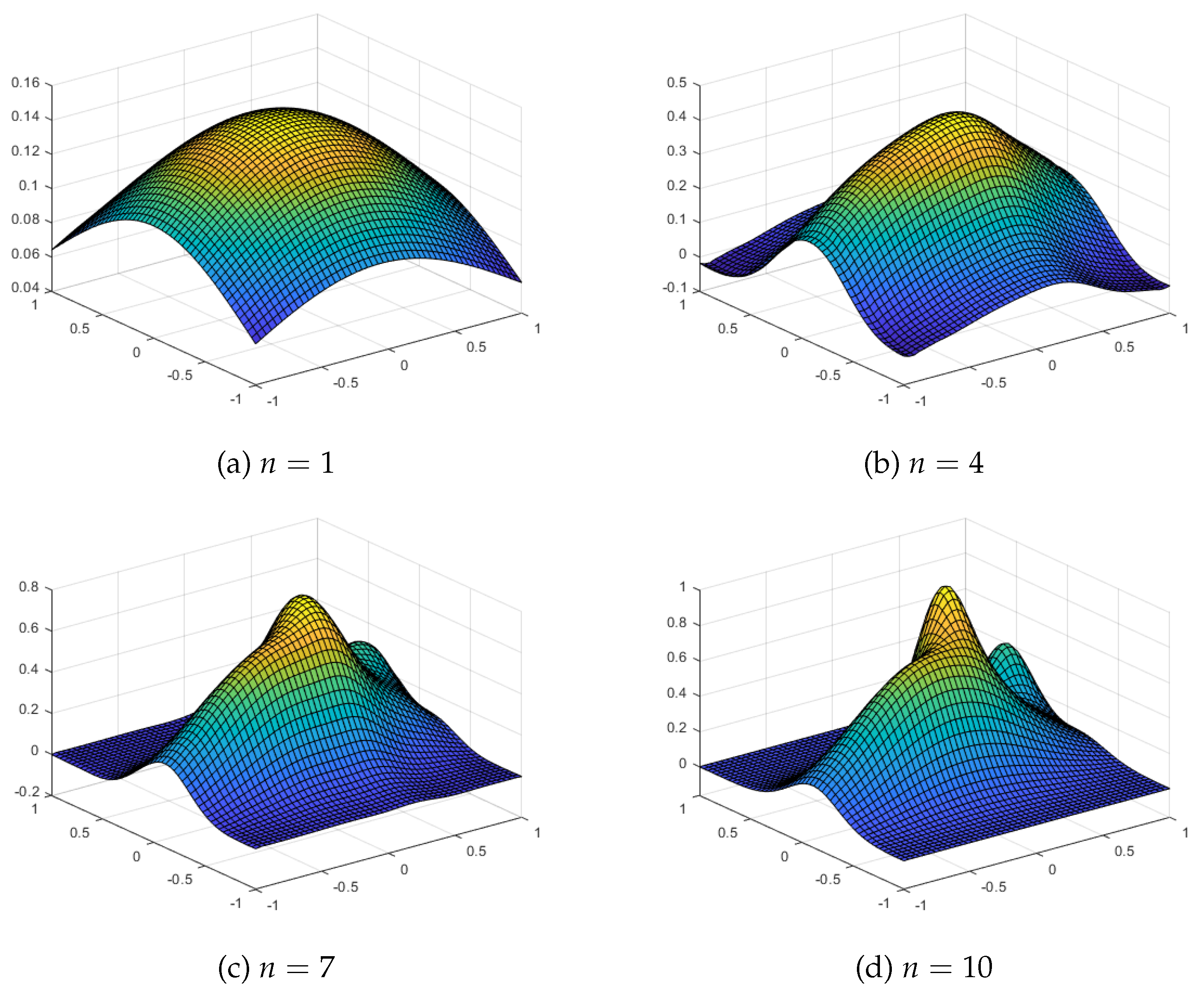
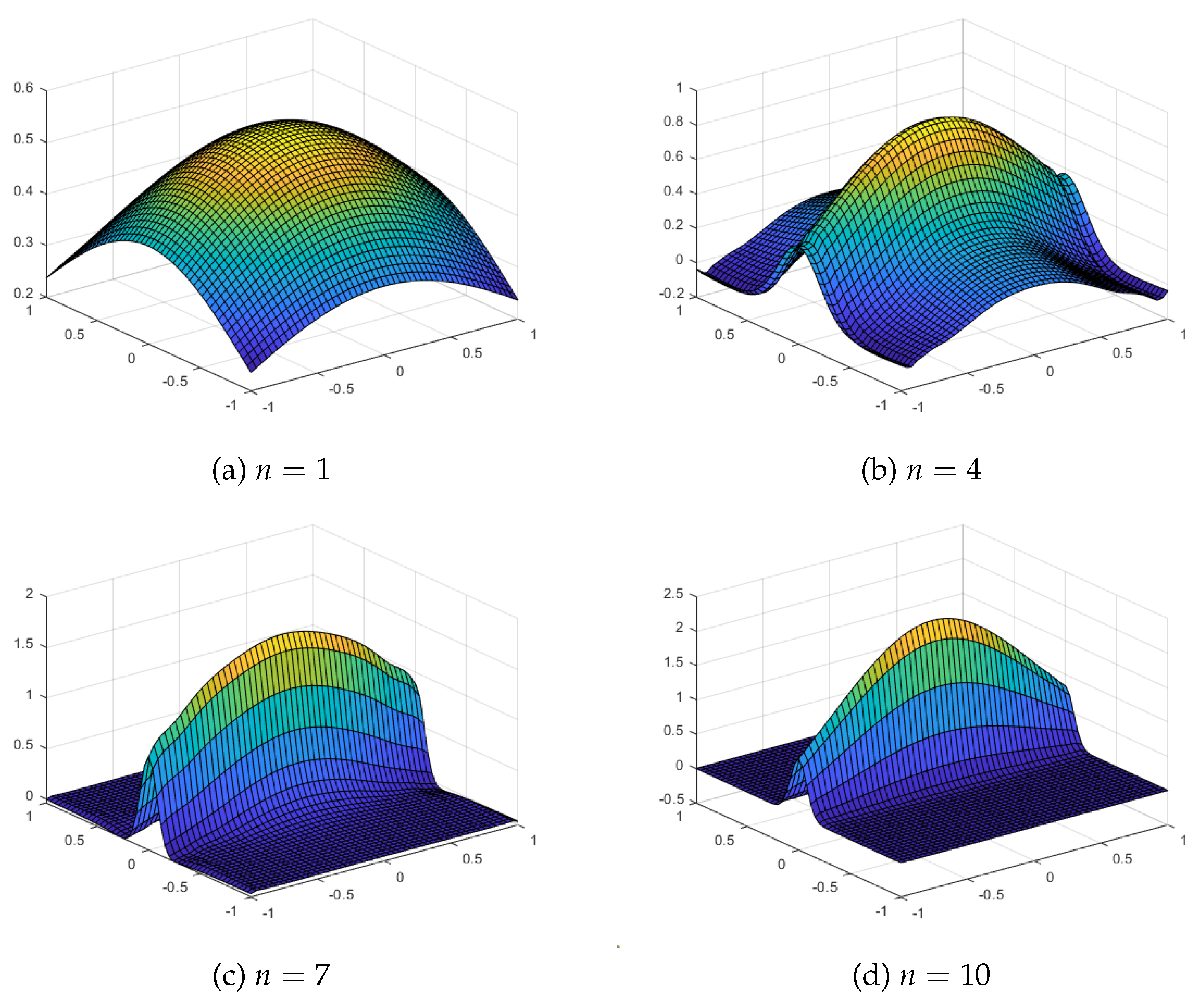
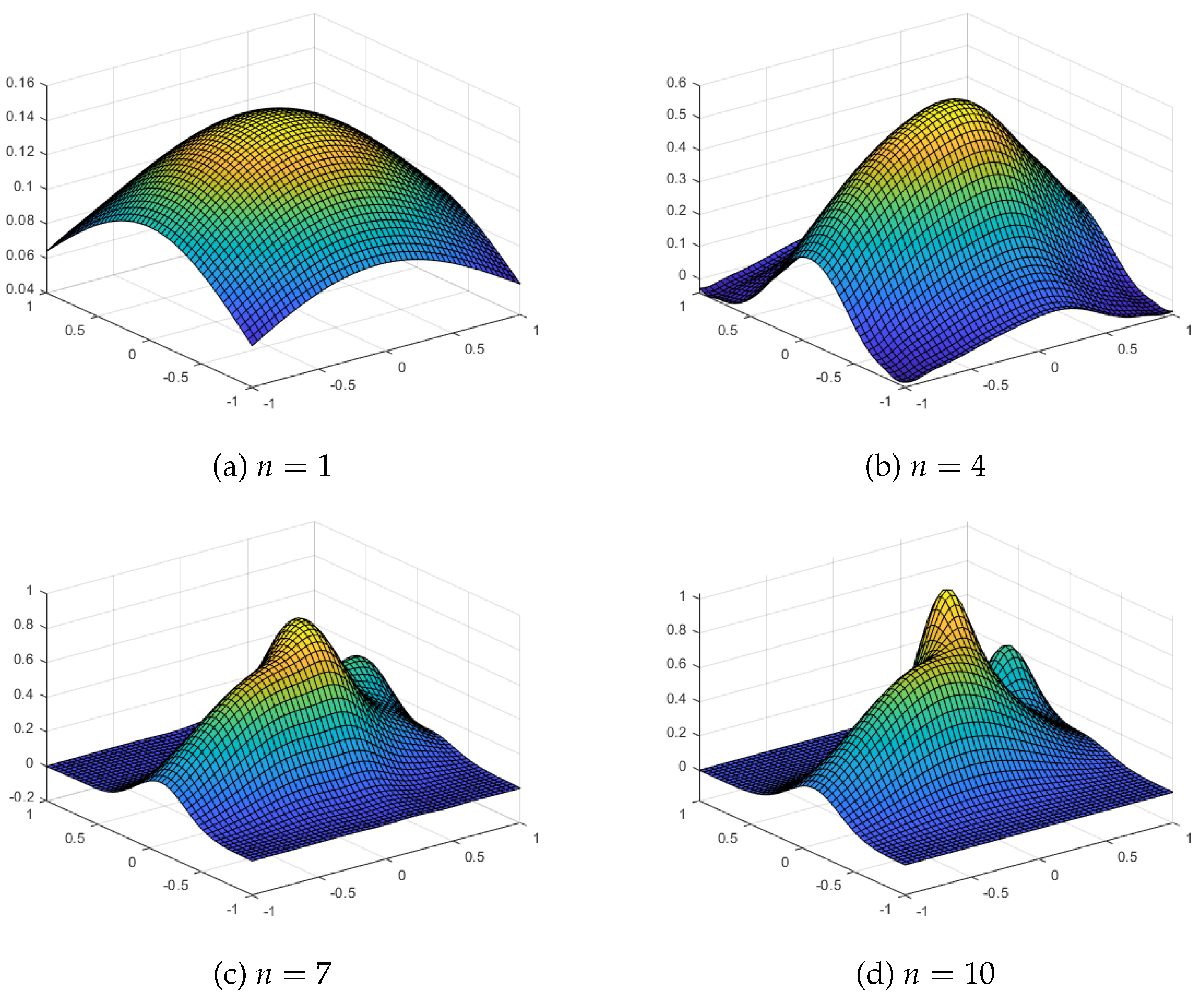
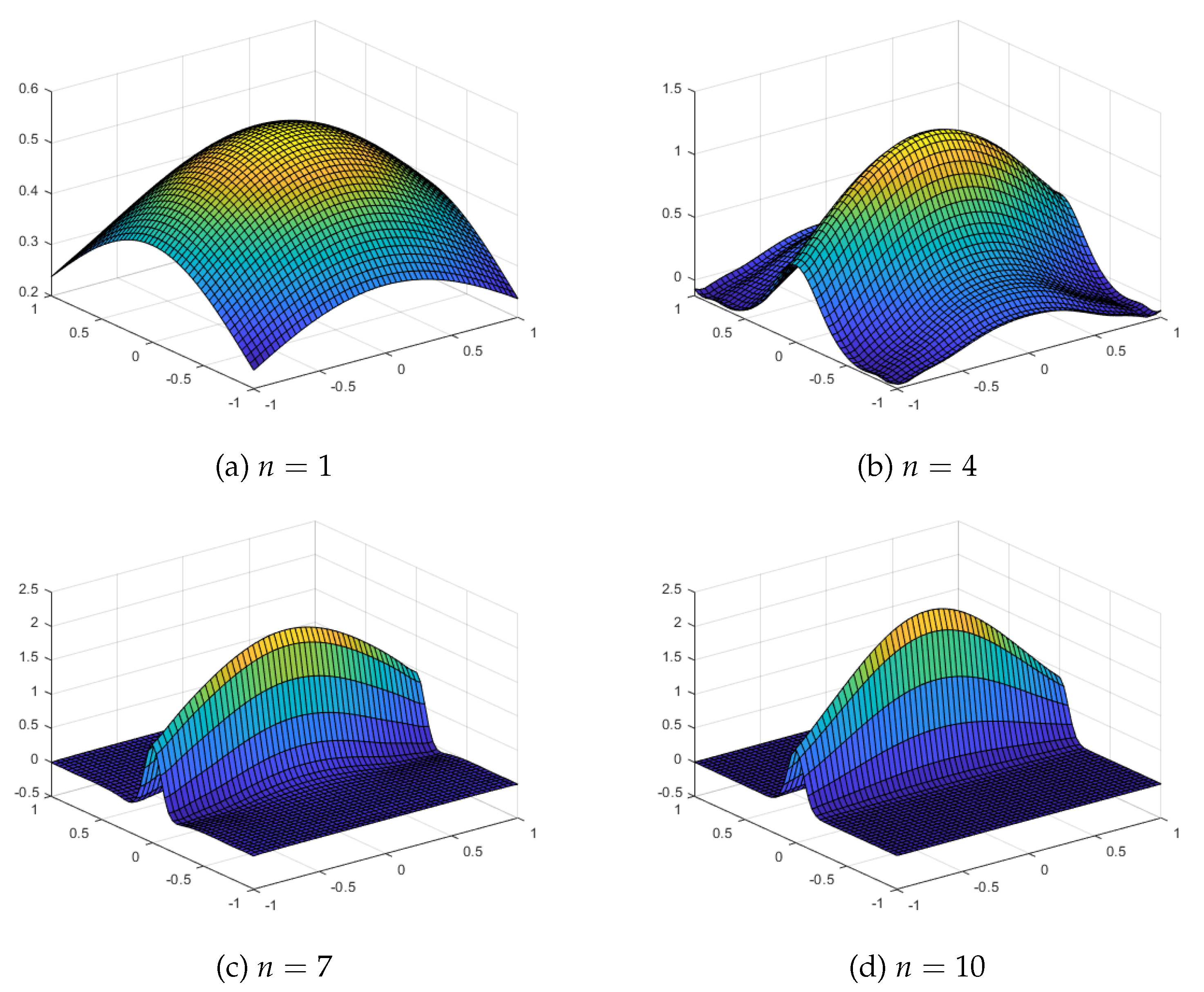
Figure 6 shows the approximation using our proposed quasi sparse kernel based interpolation with equally spaced grid

{\tilde{G}}_{n, 2}

for different values of n. Table 1 also shows the error estimates. We observe that the Max Error or the RMS error does not decreases substantially as we increase the sparse grid level n, but the plots show that approximations are very close to the true function

F_{1}^{2 d}

for

n > 6

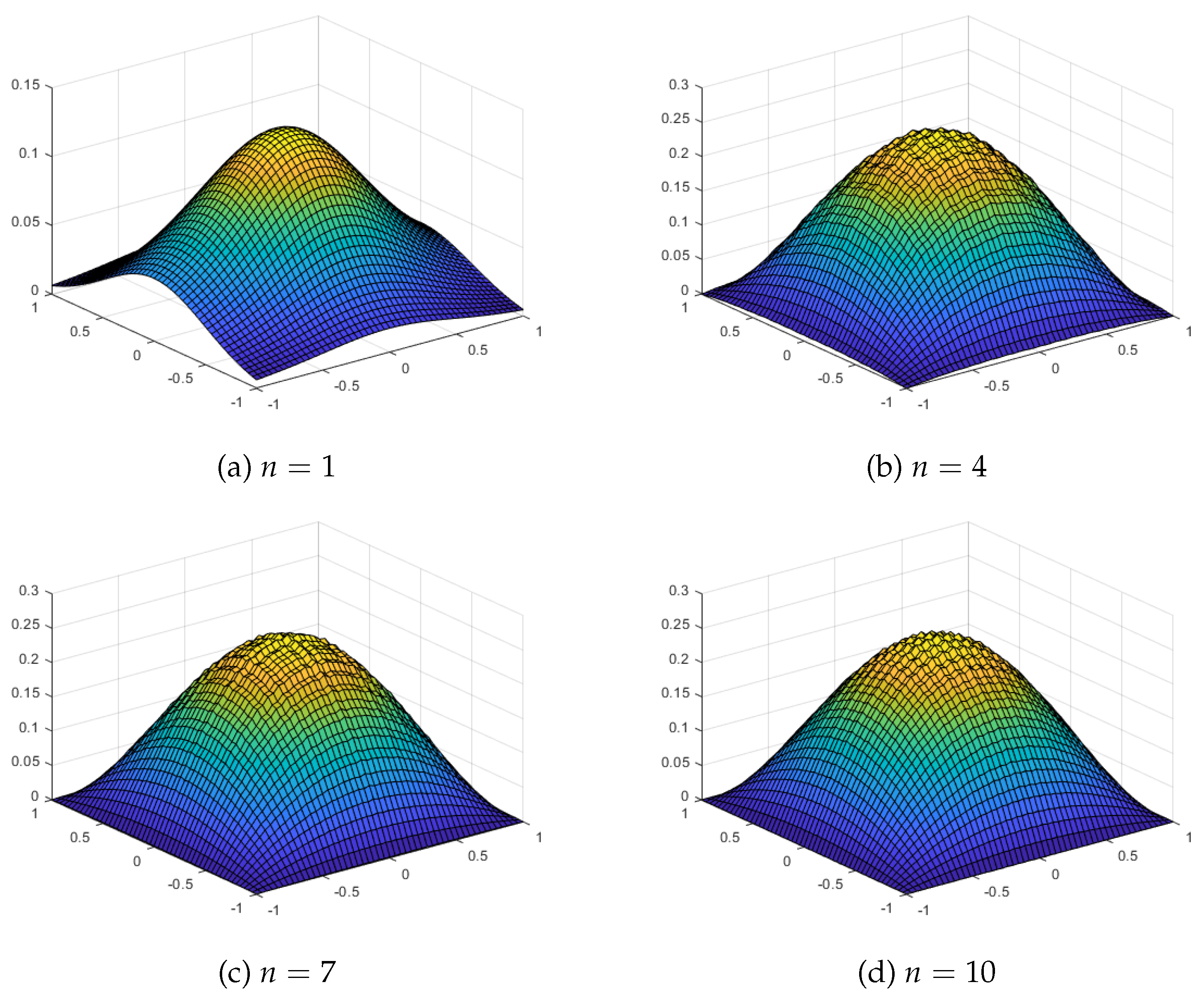
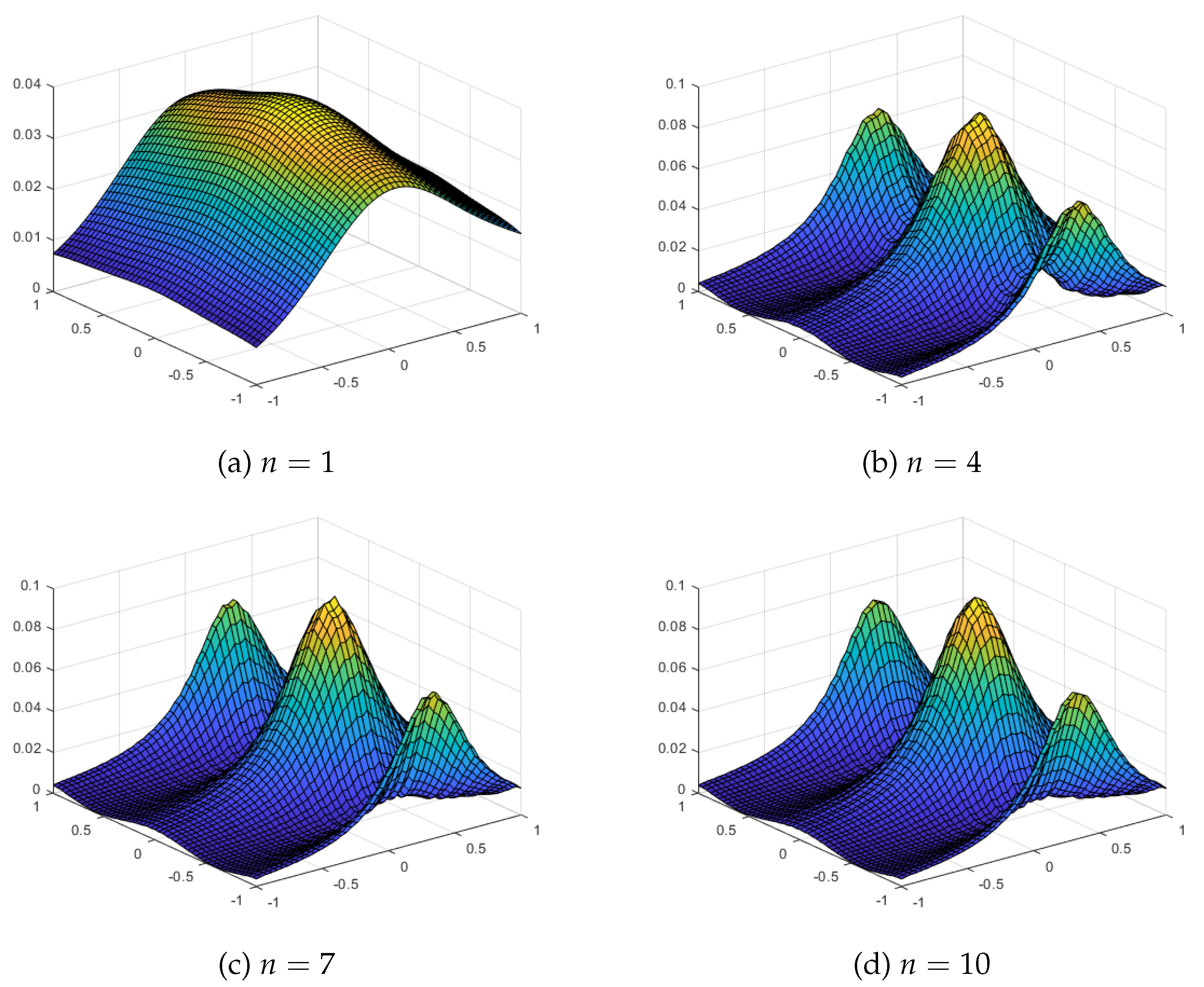
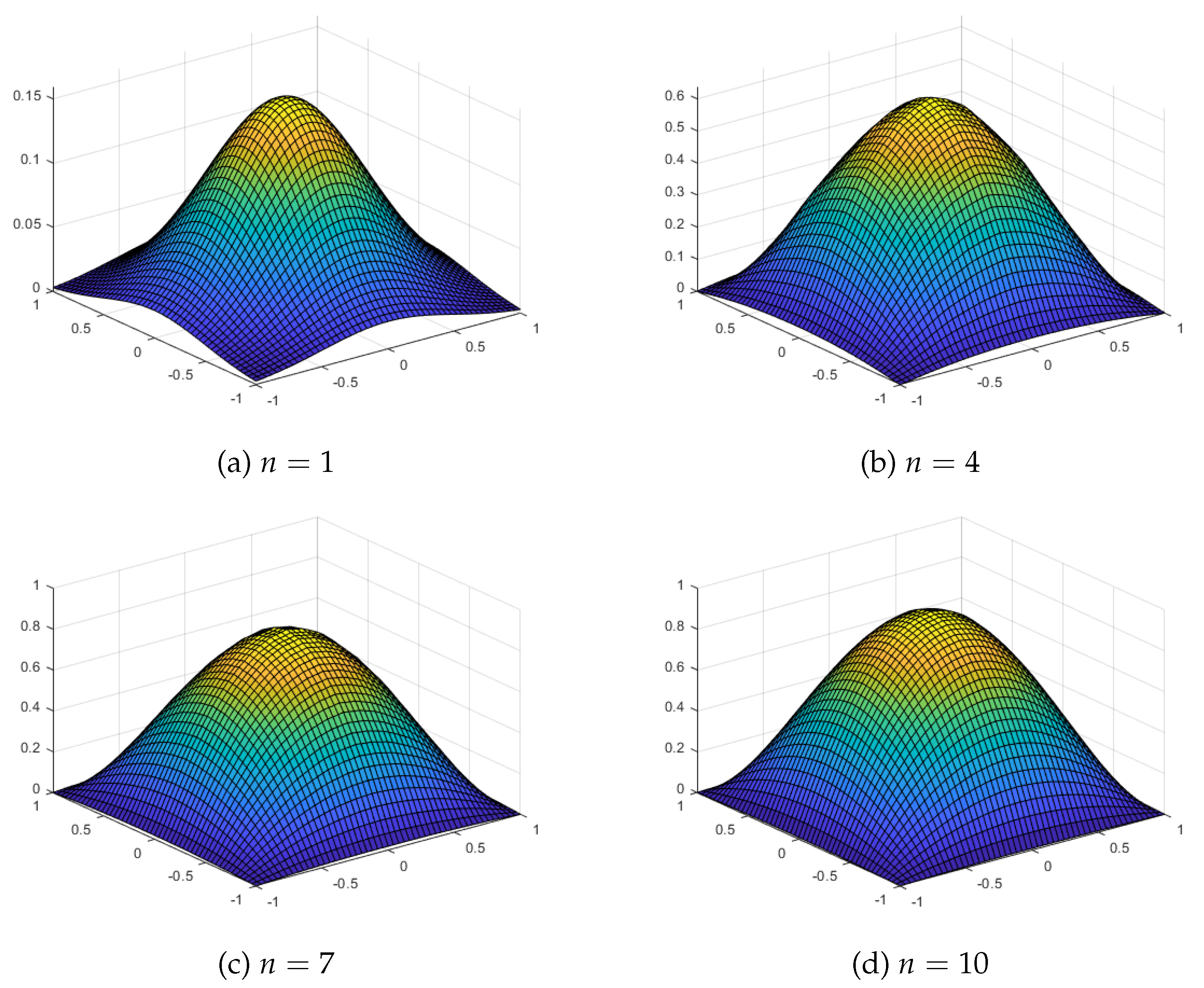
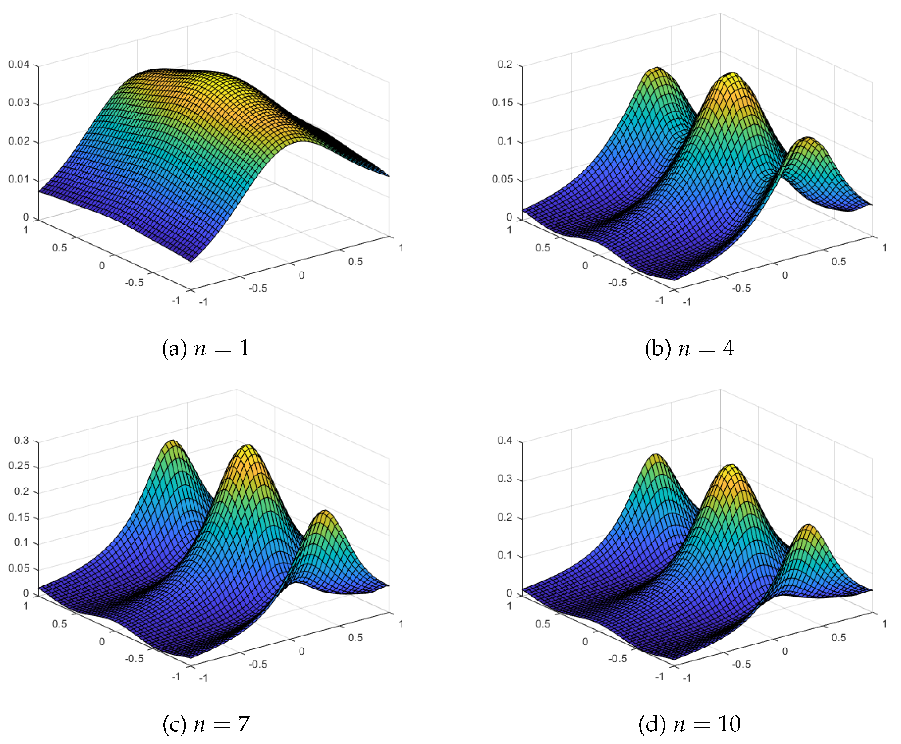
. With the Chebyshev points, we observe much better approximations with both Max Error and the RMS Error decreasing with the increase in level n. The plots of the interpolating function evaluated at the

50 \times 50

grid points for the algorithm with Chebyshev points are shown in Figure 7. We again observe that the approximations are quite good for

n > 6

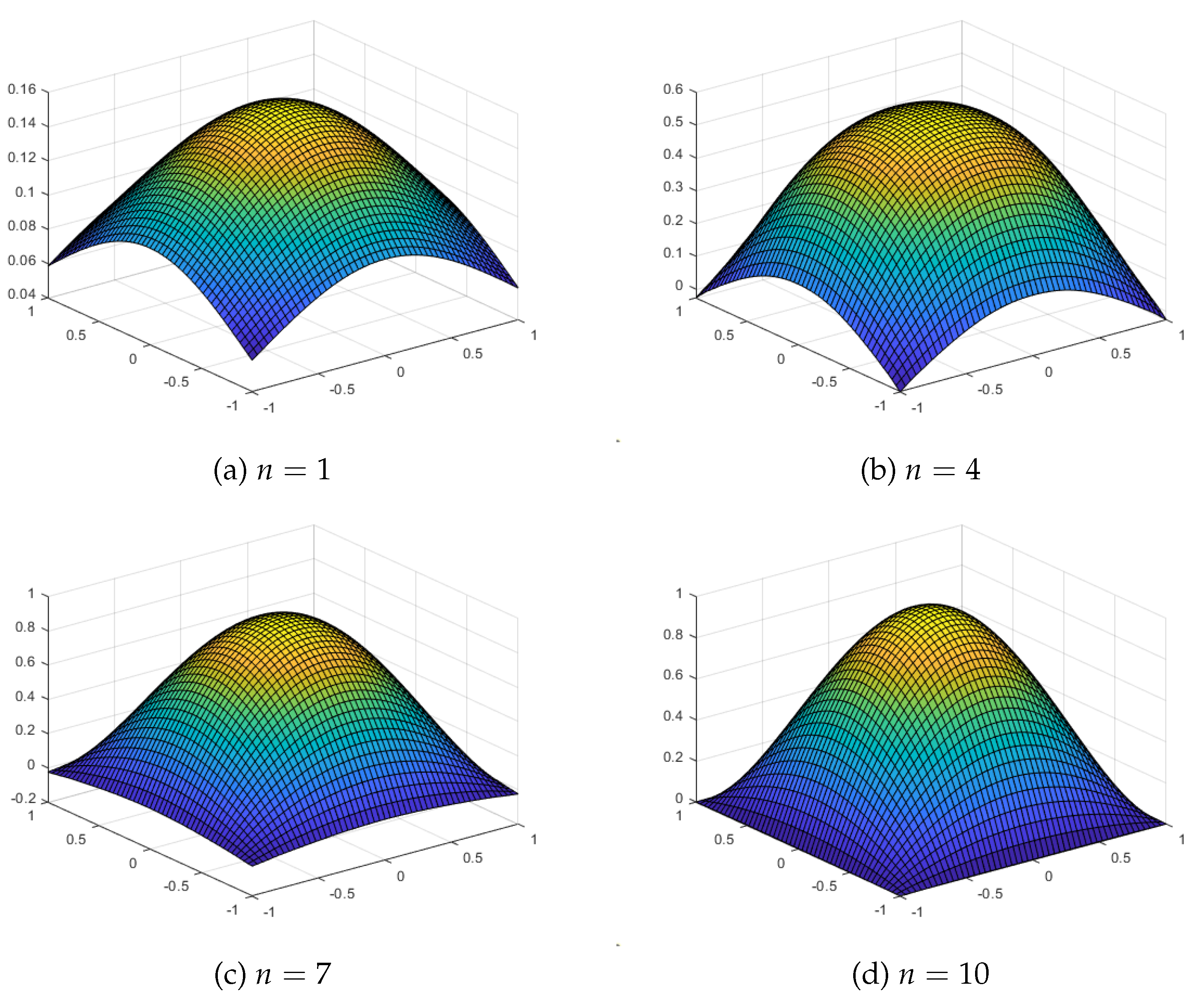
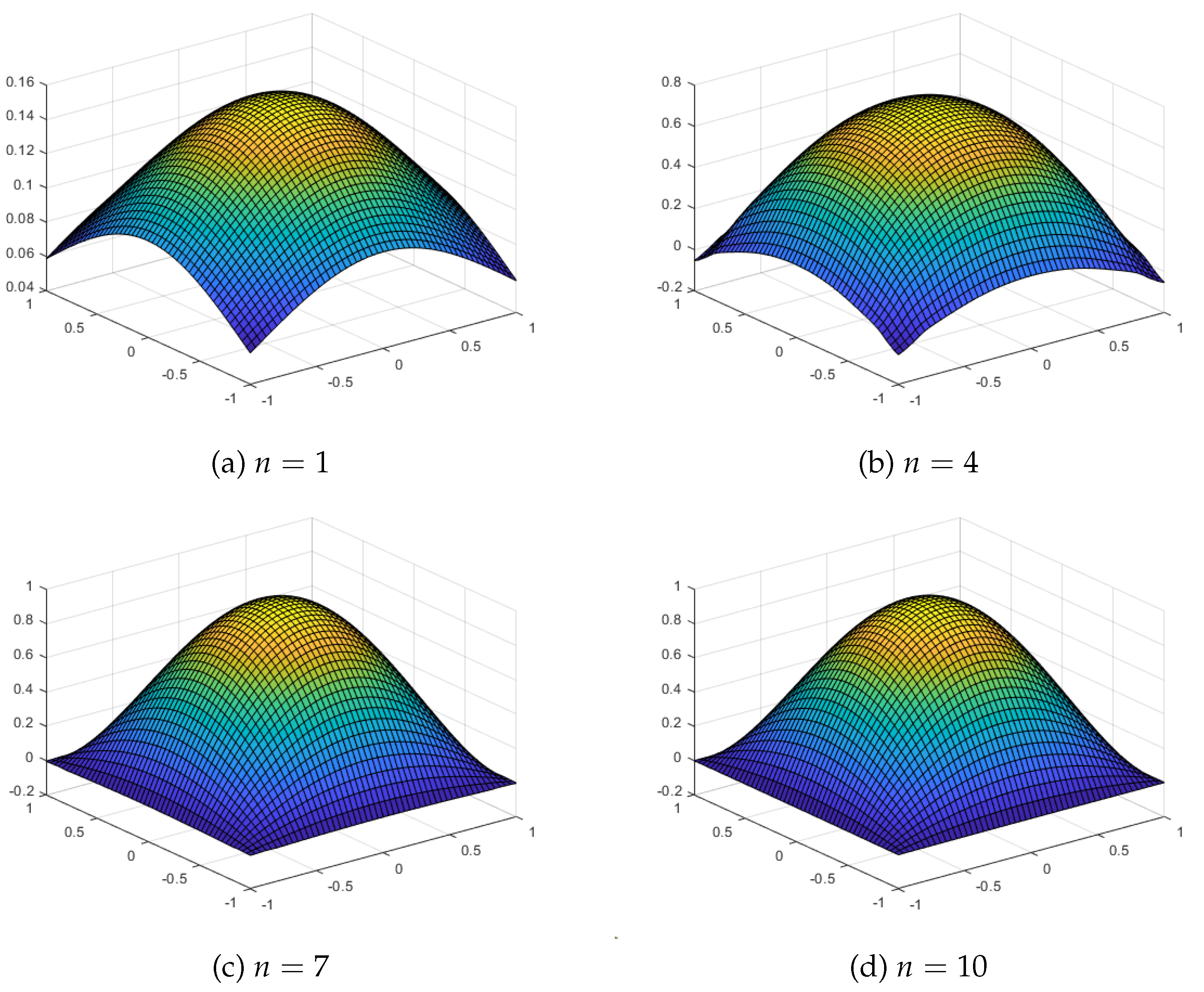
Figure 8 shows the approximations using our proposed quasi sparse kernel based interpolation with equally spaced grid

{\tilde{G}}_{n, 2}

for different values of n for the test function

F_{2}^{2 d} (x, y)

. Table 2 also shows the error estimates. We observe that the Max Error or the RMS error does not decreases substantially as we increase the grid level n, but the plots show that approximations are very close to the true function

F_{2}^{2 d}

for

n > 2

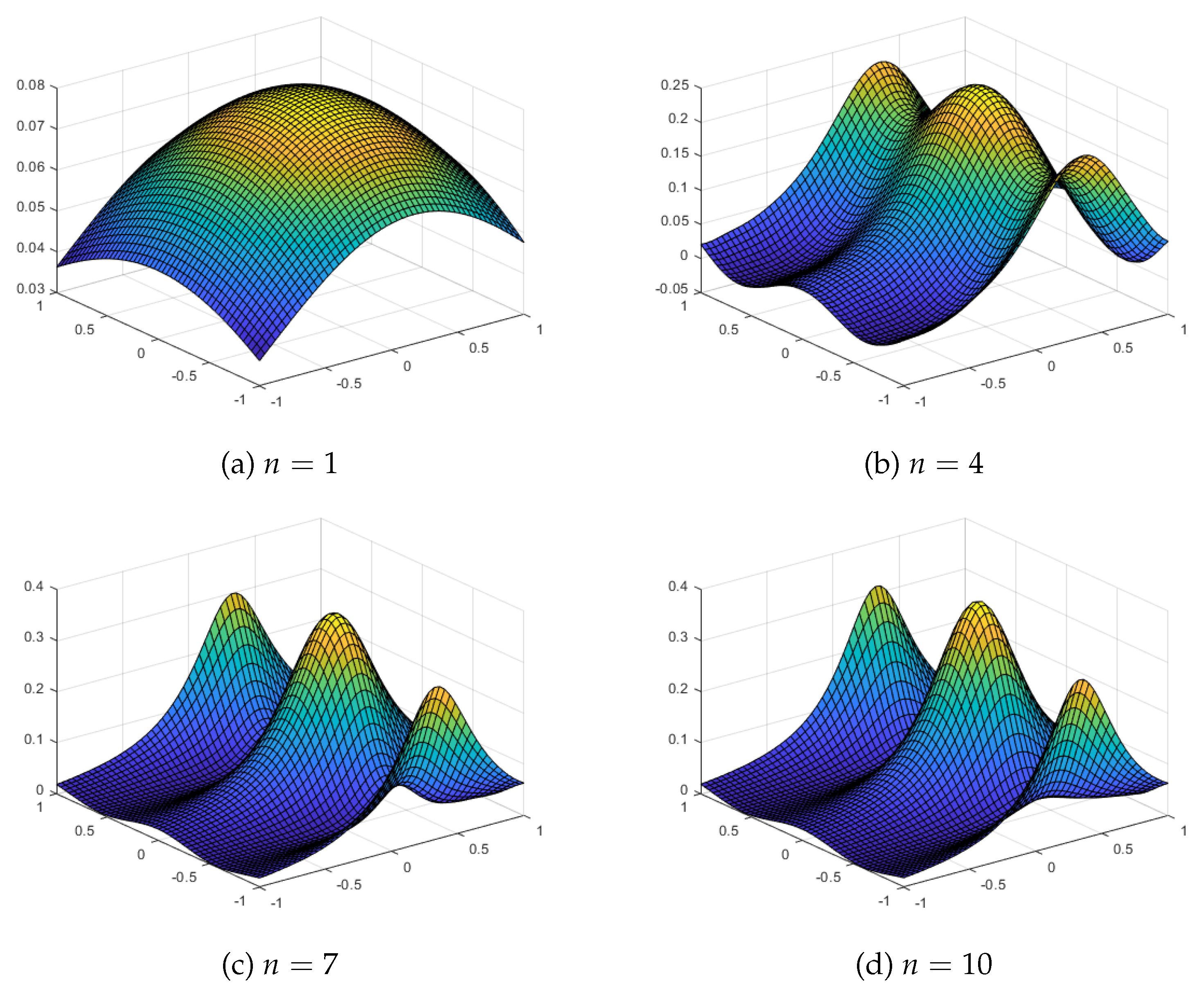
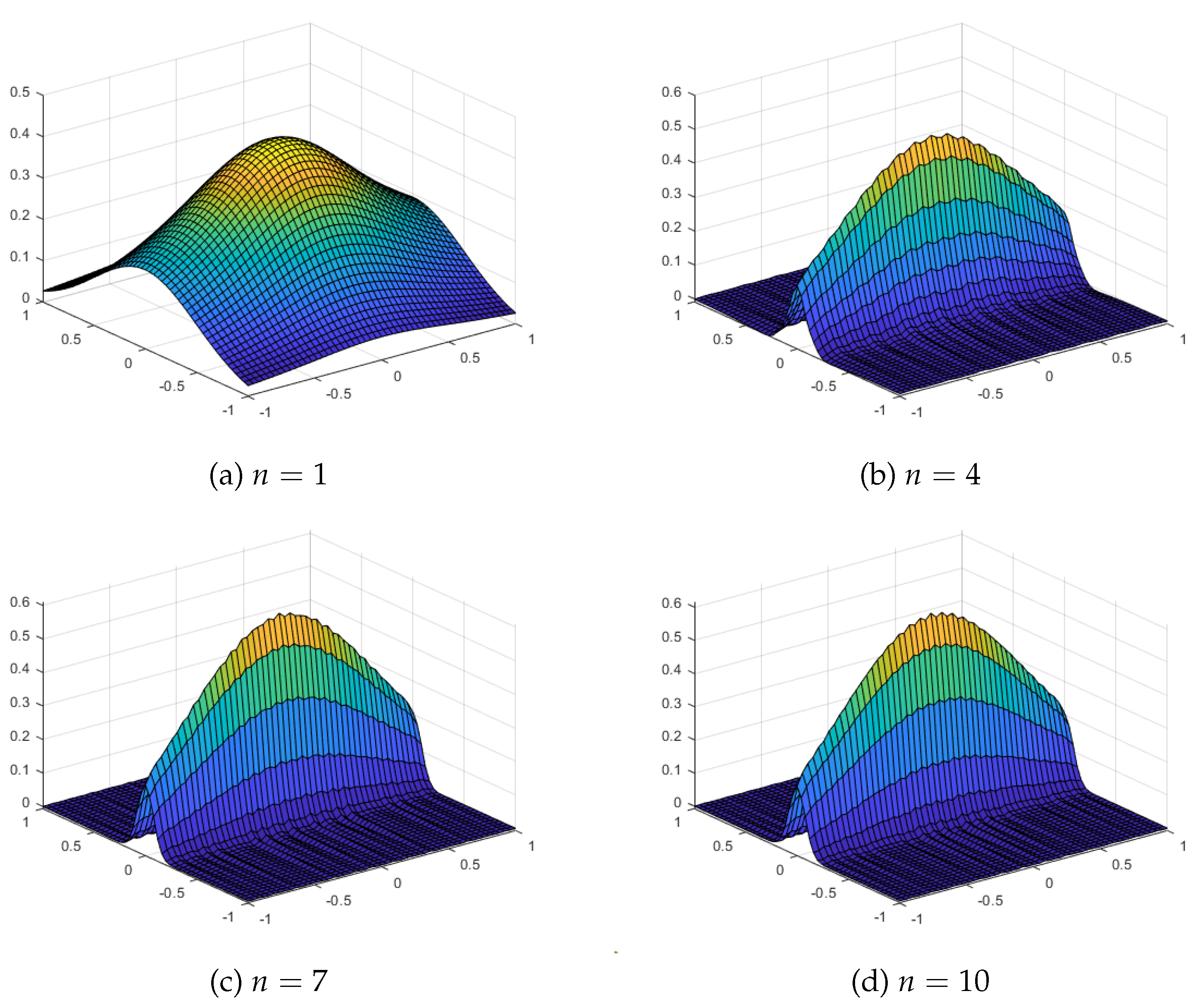
when we have used equally spaced grids. With the Chebyshev points, we observe much better approximations with both Max Error and the RMS Error decreasing with the level n. The plots of the interpolating function evaluated at the

50 \times 50

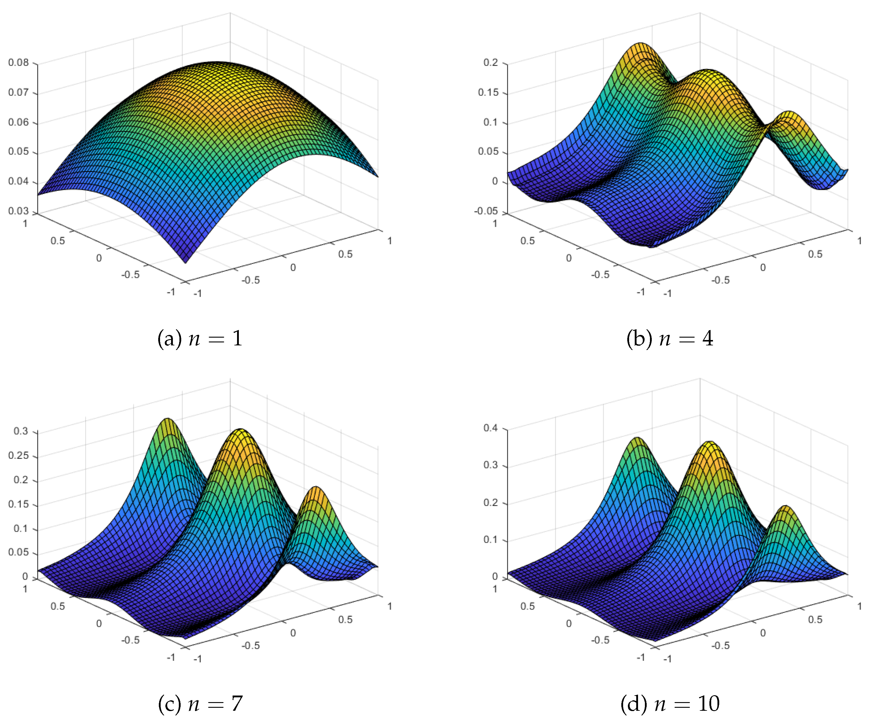
grid points for the algorithm with Chebyshev points are shown in Figure 9. For

n = 1

, the approximations are poor, but it approximates nicely as n increases. On the other hand, when there are equally spaced grid, the interpolant starts to overfit the surface and lacks smoothness for the larger values of n. Thus, by increasing the number of grid level, the approximation actually deteriorates for the equally spaced grids.

Figure 10 shows the approximations using our proposed quasi sparse kernel based interpolation with equally spaced grid

{\tilde{G}}_{n, 2}

for different values of n for the test function

F_{3}^{2 d} (x, y)

. Table 3 also shows the error estimates. We observe that the Max Error or the RMS error does not decrease substantially as we increase the grid level n, but the plots show that approximations are very close to the true function

F_{3}^{2 d}

for

n > 4

50 \times 50

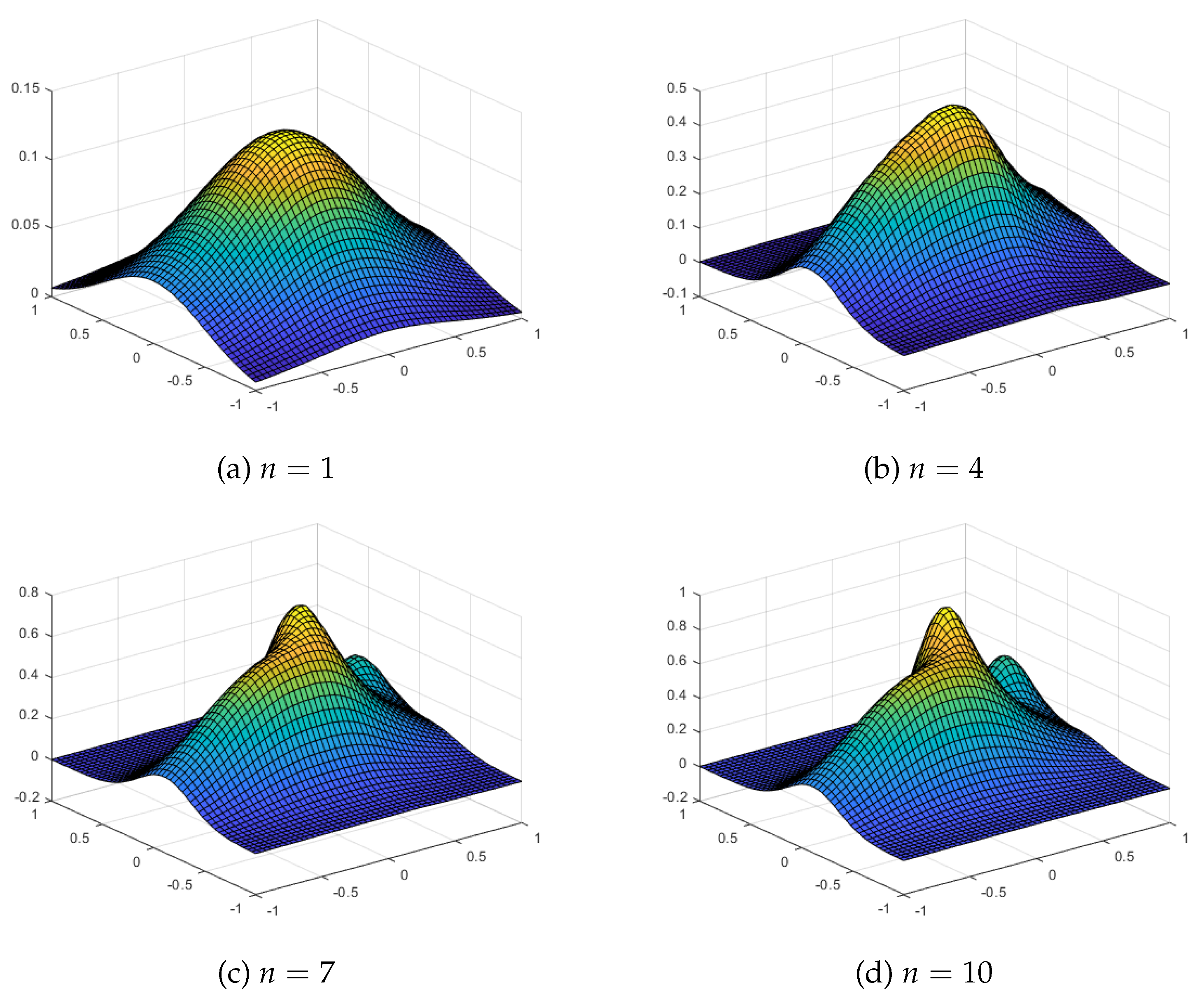
grid points for the algorithm with Chebyshev points are shown in Figure 11. For

n = 1

, the approximations are poor and the overall shape is not similar to the shape of the function, but it approximates nicely as n increases. On the other hand, when there are equally spaced grid, the interpolant starts to overfit the surface and lacks smoothness for the larger values of n. Thus, by increasing the number of grid level, the approximation actually deteriorates for the equally spaced grids.

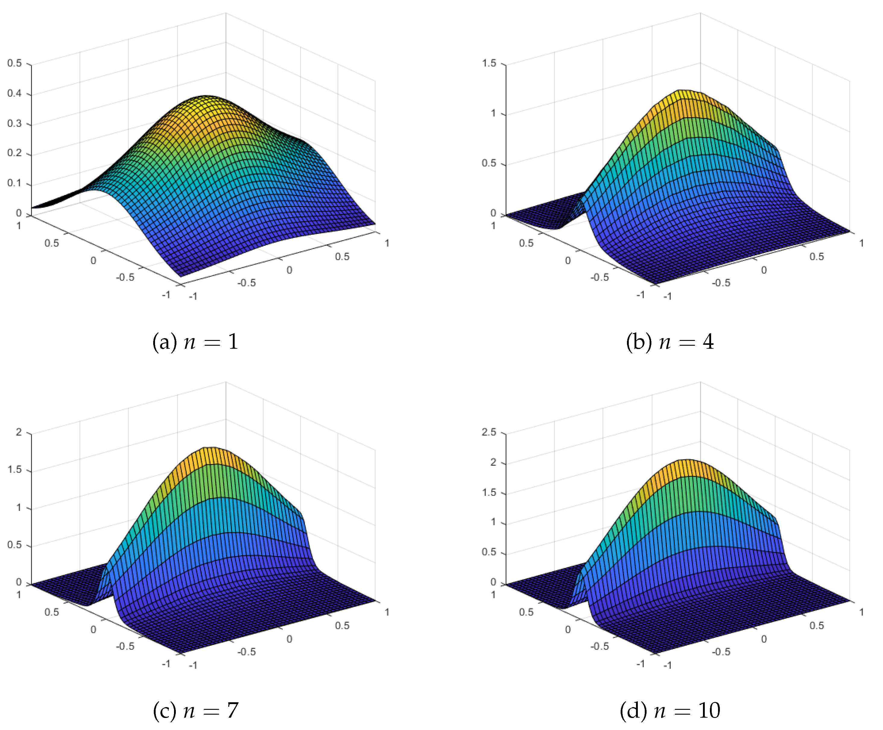
Figure 12 shows the approximations using our proposed quasi sparse kernel based interpolation with equally spaced grid

{\tilde{G}}_{n, 2}

for different values of n for the test function

F_{4}^{2 d} (x, y)

. Table 4 also shows the error estimates. We observe that the Max Error or the RMS error does not decrease substantially as we increase the grid level n, but the plots show that approximations are very close to the true function

F_{4}^{2 d}

for

n > 4

50 \times 50

grid points for the algorithm with Chebyshev points are shown in Figure 13. For

n = 2

, the approximations are poor and the overall shape is not similar to the shape of the function, but it approximates nicely as n increases.

In these results, quasi-sparse interpolation with equally space grids has reached the stable maximum absolute error and the root mean square errors at a lower level with a small number of sparse grid points. However, the quasi-sparse interpolation with Chebyshev points attain much smaller values for maximum errors and the RMS errors for all test functions and stabilizes for a larger values of the level n. Additionally, since the errors remain stable when the number of grid-points increases, the quasi-sparse interpolation goes well with the multilevel quasi sparse algorithm, which will be examined in a subsequent sub-section. The main observation, in these results s that the quasi-sparse interpolation does not converge for equally spaced grids but they do converge for Chebyshev grid points. The rate of convergence depends on the test function.

7. Numerical Experiments for Quasi-sparse Interpolations with $d = 3$

In this section, we present some performance analysis for some test functions with domain

Ω = {[- 1, 1]}^{3}

in dimension

d = 3

. Following functions are used as test functions:

$F_{1}^{3 d} (x, y)$ (Franke’s function)

$\begin{matrix} F_{1}^{3 d} (x, y) & = & 0.75 e^{- ({(9 x - 2)}^{2} + {(9 y - 2)}^{2} + {(9 z - 2)}^{2}) / 4} + 0.75 e^{- {(9 x + 1)}^{2} / 49 - {(9 y + 1)}^{2} / 10 - {(9 z + 1)}^{2} / 10} \\ + 0.5 e^{- ({(9 x - 7)}^{2} + {(9 y - 3)}^{2} + {(9 z - 5)}^{2}) / 4} - 0.2 e^{- ({(9 x - 4)}^{2} + {(9 y - 7)}^{2} + {(9 z - 5)}^{2})} . \end{matrix}$
$F_{2}^{3 d} (x, y) = (1 - x^{2}) (1 - y^{2}) (1 - z^{2})$ .
$F_{3}^{3 d} (x, y) = \sqrt{\frac{18}{π}} e^{- (x^{2} + 81 y^{2} + z^{2})}$ .
$F_{4}^{3 d} (x, y) = cos (6 z) \frac{1.25 + cos (5.4 y)}{6 + 6 {(3 x - 1)}^{2}}$ .

The performance of our quasi-sparse kernel based interpolant are evaluated in a grid of

20 \times 20 \times 20

equally spaced points in the cube

{[- 1, 1]}^{3}

. The results are summarised in Table 5,Table 6,Table 7,Table 8. Due to large computing time and unavailability of parallel computing environment, we evaluate only

n = 7

levels for the multilevel algorithm. The results are similar to our observation for the numerical experiments in

d = 2

as we do not observe any convergence of the quasi-sparse interpolation with equally spaced grids but the approximations converge for Chebyshev points in all test functions.

8. Numerical Experiments for Multilevel Quasi-Sparse Interpolation

In this section, we illustrate the performance of our proposed multilevel quasi sparse kernel based interpolation method for the same test functions

F_{1}^{2 d}

F_{2}^{2 d}

F_{3}^{2 d}

and

F_{4}^{2 d}

as introduced earlier. We have evaluated the interpolations at a grid of

50 \times 50

points in the rectangle

[- 1, 1] \times [- 1, 1]

. The results are shown in Table 9,Table 10,Table 11,Table 12 for the tests functions in

d = 2

. Some of the approximate functions are also plotted in Figure 14,Figure 15,Figure 16,Figure 17,Figure 18,Figure 19,Figure 20.Figure 21. For both equally spaced sparse grid and the Chebyshev points based sparse grids, we observe that the Max Error and the root-mean-square error decreases with the increase in level n. The multilevel quasi-sparse interpolation results are even better with Chebyshev points instead of equally spaced grids.

Next, we illustrate the application of our multilevel quasi sparse interpolation with Gaussian kernel for the test functions

F_{1}^{3 d}

F_{2}^{3 d}

F_{3}^{3 d}

and

F_{4}^{3 d}

in dimension

d = 3

as introduced earlier. For

d = 3

, we have evaluated the multilevel interpolation at a grid of

20 \times 20 \times 20

points in the cube

{[- 1, 1]}^{3}

. Table 13,Table 14,Table 15,Table 16 show the error estimates with maximum absolute error and root mean square errors for the proposed interpolant for levels upto

n = 7

. We again observe that the errors decrease with the level n for the multilevel procedure for both equally spaced grids and the Chebyshev points. However, the errors are much smaller for the Chebyshev points for higher levels.

9. Convergence with Computation Time

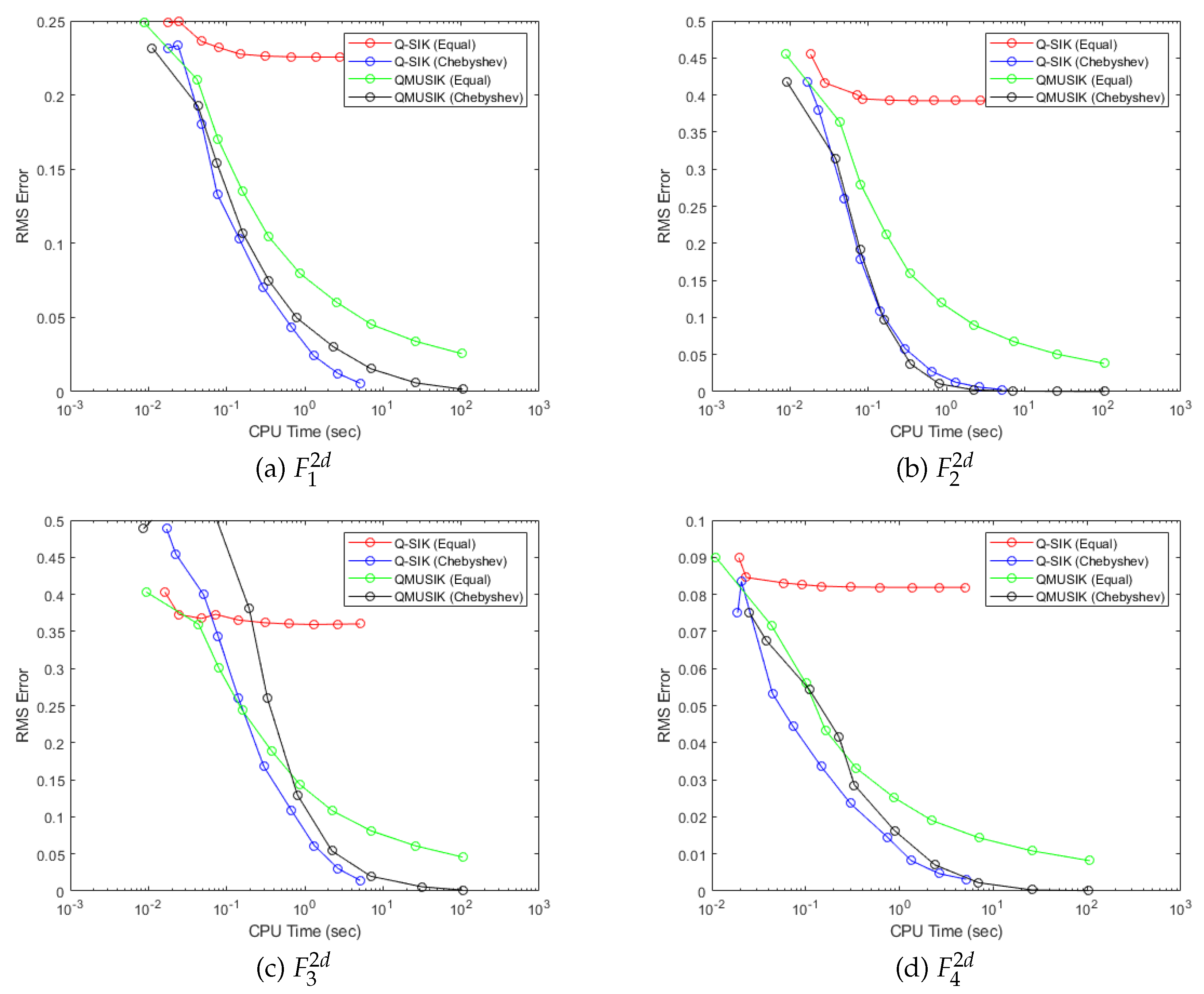
In Figure 22, root mean square (RMS) error is plotted against the computation time for the same test functions in

d = 2

and similar plots of RMS Error against time for the test functions in

d = 3

are plotted in Figure 23. These figures show that the quasi-sparse interpolation with equally spaced grids do not converge in errors as computational time increases.On the other hand, the errors decreases quite fast for quasi-sparse interpolation with Chebyshev points and converges. The multilevel quasi-sparse interpolation with equally spaced grid improves the errors in approximation and shows some convergence, but still Chebyshev points have a lot better convergence results than equally spaced points. It is also interesting to note that at a similar computational time (in seconds), quasi-sparse interpolation with Chebyshev points yield better results than the multilevel method, though multilevel methods execute only at a smaller number of levels at a comparable time.

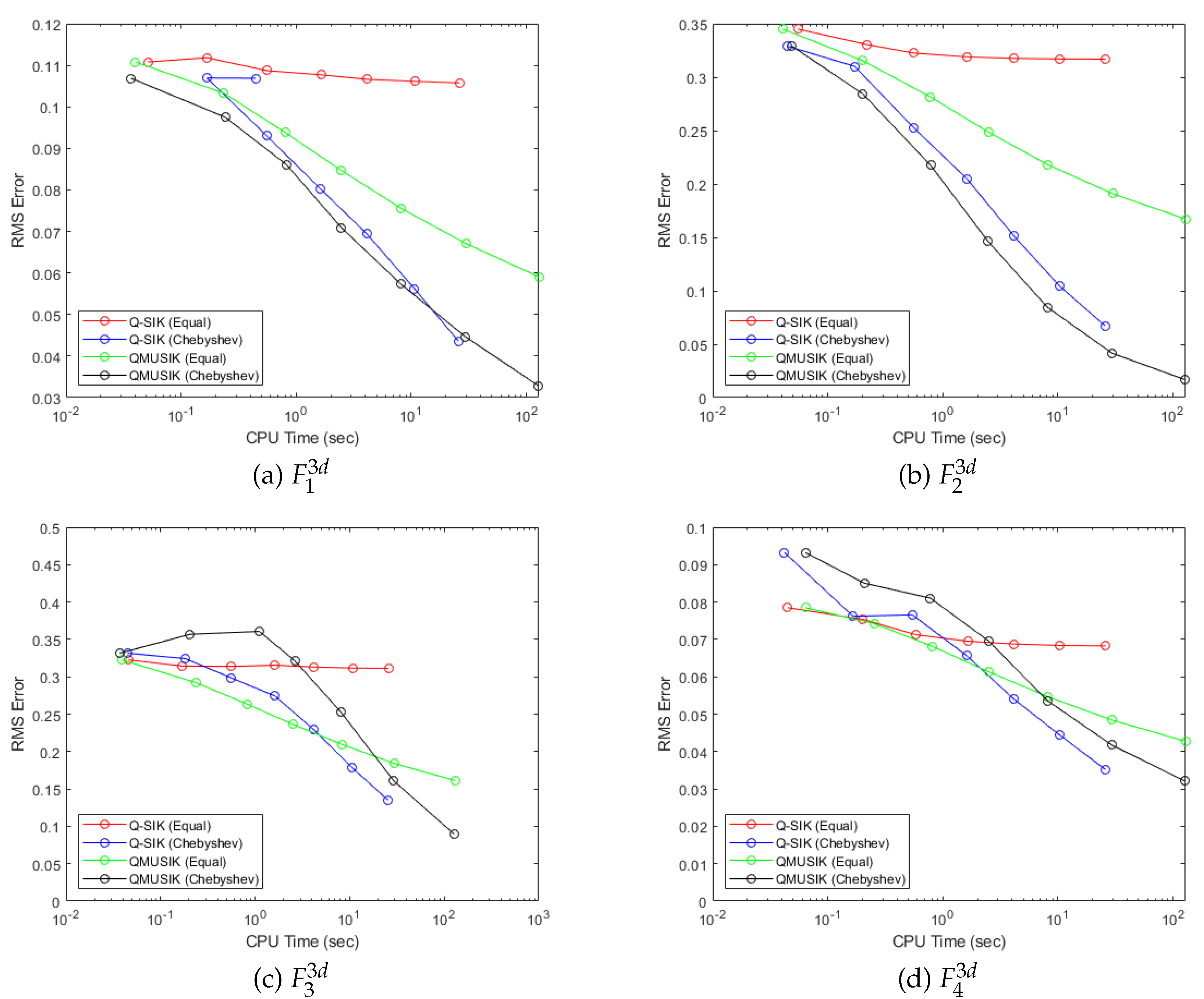
Figure 23 shows the RMS error in approximation against the computational time (in seconds) for the test functions in dimension

d = 3

. Here we do not observe the onvergence in any of the algorithms as all except equally spaced points with quasi-sparse interpolation are showing a decreasing trend in the errors with computational time. Here also, the better performance are obtained for Chebyshev points and Chebyshev points with only quasi-sparse interpolations are competitive with multilevel algorithm for a similar computational time and better than multilevel algorithm with equally spaced points.

10. Discussion and Finding

In this article, we have explored an algorithm for quasi interpolation with Gaussian kernel based on sparse grids. We have observed that quasi sparse kernel based interpolation approximates the 2 and 3 dimensional functions quite reasonably. However, the quasi interpolation is not guaranteed to converge. We have observed that even for large values of the level n of the grids, the root-mean-square error of the approximation are not converging to 0 if we use equally spaced sparse grids. However, if we use Chebyshev points the root-mean-square of the approximation steadily decreases with level n. We get much better approximation with Chebyshev points than equally spaced grid for larger values of n. However, Chebyshev points are more dense along the boundary of the domain and more sparse in the centre. For this reason, Chebyshev points yield a very poor approximation in the centre for smaller values of n, which is evident from the plots with Chebyshev approximations with

n = 1

n = 2

The way the grids

G_{ℓ}

are constructed, it is possible to implement the algorithm in parallel to make it faster. Otherwise, the repeat of evaluation of the anisotropic interpolant at many grid points for different values of n slows down the execution. We can see that for

d = 2

, the level

n = 10

has 13313 distinct points only but these points are revisited many time yielding a total number of points used for computation to be 35851. This increases the function evaluation by nearly 3 times. For

d = 3

and the level

n = 7

, the number of unique grid points is 8961 only, but the points used for computation is 38868. Due to this, the time complexity of the algorithm increases many fold, one should either implement the algorithm for parallel computing only or should improve the algorithm to avoid revisiting the grid points for different multi-index ℓ.

In this article, we have also proposed the multilevel quasi sparse kernel based interpolation based on equally spaced grids as well as sparse grids based on Chebyshev points. We illustrated our proposed methods using some test functions numerically. We observed that the proposed multilevel quasi procedure performs better than the quasi sparse interpolation proposed. However, the computational time for the multilevel method is considerably higher than the simple quasi sparse interpolation. This is because the multilevel method requires the residual functions to be evaluated at every sparse grid points and as the level n increase, the number of sparse grid points also increases exponentially and that leads to a huge increase in computational time. On a positive note, we would like to mention that due to the nature of the sparse grid construction, it is possible to implement the algorithm for parallel computing and that will reduce the computational time considerably.

Furthermore, multilevel quasi sparse algorithm requires substantially less computational time compared to other multilevel methods proposed in the literature as it does not require to solve a system of linear equations at every level of approximations with the residual functions. Due to the implementation of the quasi sparse algorithm at every level, the proposed multilevel quasi sparse method will have linear time complexity with the level n.

11. Conclusion

The paper has successfully demonstrated the viability and advantages of using multilevel quasi-interpolation techniques on Chebyshev sparse grids. In comparison to conventional methods, the multilevel quasi-sparse interpolation with Gaussian kernels showed promising performance metrics. This paper also elaborated on the implementation complexities and challenges, providing an efficient way to construct sparse grids and compute anisotropic quasi-interplants. While the methodology was effective in lower dimensions two dimension and three dimension, limitations began to appear as computational time and complexity increased, indicating areas for future research and optimisation.

The numerical experiments yielded insightful data on the performance of this technique, showcasing its capacity for faster convergence with computation time in specific settings. The study acts as a foundational resource for future research aiming to employ multilevel quasi-interpolation techniques for various applications, especially in high-dimensional computational problems.

Funding

This research received no external funding.

Data Availability Statement

No new data were created or analyzed in this study. Data sharing is not applicable to this article

Acknowledgments

The author thankful to the University of Leicester for providing the academic environment and resources. Additionally, sincere appreciation goes to his supervisors, Ruslan Davidchack and Jeremy Levesley, for their invaluable guidance and mentorship. Special thanks are also extended to Taibah University for their generous financial support throughout his doctoral studies.

Conflicts of Interest

The author declare no conflict of interest.

References

Alsharif, F. Multilevel Quasi-Interpolation With a Gaussian Kernel using Chebyshev Points - Numerical and theoretical studies using the radial basis function approach 2023. [CrossRef]
Alsharif, F. Quasi-Interpolation on Chebyshev Grids with Boundary Corrections. Computation 2024, 12. [Google Scholar] [CrossRef]
Franz, T.; Wendland, H. Multilevel quasi-interpolation. IMA Journal of Numerical Analysis 2022. [Google Scholar] [CrossRef]
Georgoulis, E.; Levesley, J.; Subhan, F. Multilevel sparse kernel based interpolation. SIAM Journal of Scientific Computing 2013, 35, 815–832. [Google Scholar] [CrossRef]
Beatson, R.; Powell, M. Univariate multiquadric approximation: quasi-interpolation to scattered data. Constr. Approx 1992, 8, 275–288. [Google Scholar] [CrossRef]
Wu, Z.; Robert, S. Shape preserving properties and convergence of univariate multiquadric quasi-interpolation. Acta Mathematicae Applicatae Sinica 1994, 10, 441–446. [Google Scholar] [CrossRef]
Wu, Z.; Liu, J. Generalized strang-fix condition for scattered data quasi-interpolation. Adv. Comput. Math 2005, 23, 201–214. [Google Scholar] [CrossRef]
Floater, M.S.; Iske, A. Multistep scattered data interpolation using compactly supported radial basis functions. J. Comput. Appl. Math 1996, 73, 65–78. [Google Scholar] [CrossRef]
Hales, S.J.; Levesley, J. Error estimates for multilevel approximation using polyharmonic splines. Numerical Algorithms 2002, 30, 1–10. [Google Scholar] [CrossRef]
Hubbert, S.; Levesley, J. Convergence of Multilevel Stationary Gaussian Quasi-Interpolation 2017.
Franke, R. Scattered data interpolation: tests of some methods. Mathematics of Computation 1982, 38(157), 181–200. [Google Scholar]
Fasshauer, G.E. Meshfree approximation methods with MATLAB of Interdisciplinary Mathematical Sciences. World Scientific Publishing Co. Pte. Ltd., Hackensack, NJ. volume 2007, 6. [Google Scholar]
Beatson, R.; Davydov, D.; Levesley, J. Error bounds for anisotropic rbf interpolation. Journal of Approximation Theory 2010, 162(3), 512–527. [Google Scholar] [CrossRef]
Casciola, G.; Montefusco, L.B.; Morigi, S. The regularizing properties of anisotropic radial basis functions. Applied Mathematics and Computation 2007, 190(2), 1050–1062. [Google Scholar] [CrossRef]

Figure 1. Sparse grid

{\tilde{G}}_{4.2}

Figure 1. Sparse grid

{\tilde{G}}_{4.2}

Figure 2. Sparse Chebyshev grid

{\tilde{G}}_{4.2}^{c}

Figure 2. Sparse Chebyshev grid

{\tilde{G}}_{4.2}^{c}

Figure 3. Nested nature of the sparse grids

{\tilde{G}}_{n, 2}

with equally spaced points for

n = 1, 2, \dots, 6

Figure 3. Nested nature of the sparse grids

{\tilde{G}}_{n, 2}

with equally spaced points for

n = 1, 2, \dots, 6

Figure 4. Nested nature of the sparse grids

{\tilde{G}}_{n, 2}^{c}

with Chebyshev points for

n = 1, 2, \dots, 6

Figure 4. Nested nature of the sparse grids

{\tilde{G}}_{n, 2}^{c}

with Chebyshev points for

n = 1, 2, \dots, 6

Figure 5. Test functions in two dimensions


(a) $F_{1}^{2 d}$	(b) $F_{2}^{2 d}$

(c) $F_{3}^{2 d}$	(d) $F_{4}^{2 d}$

Figure 6. Approximations using equally spaced sparse grid with level n and Gaussian kernel for the test function

F_{1}^{2 d}

Figure 6. Approximations using equally spaced sparse grid with level n and Gaussian kernel for the test function

F_{1}^{2 d}


(a) $n = 1$	(b) $n = 4$

(c) $n = 7$	(d) $n = 10$

Figure 7. Approximations using Chebyshev sparse grid with level n and Gaussian kernel for the test function

F_{1}^{2 d}

Figure 7. Approximations using Chebyshev sparse grid with level n and Gaussian kernel for the test function

F_{1}^{2 d}


(a) $n = 1$	(b) $n = 4$

(c) $n = 7$	(d) $n = 10$

Figure 8. Approximations using equally spaced sparse grid with level n and Gaussian kernel for the test function

F_{2}^{2 d}

Figure 8. Approximations using equally spaced sparse grid with level n and Gaussian kernel for the test function

F_{2}^{2 d}


(a) $n = 1$	(b) $n = 4$

(c) $n = 7$	(d) $n = 10$

Figure 9. Approximations using Chebyshev sparse grid with level n and Gaussian kernel for the test function

F_{2}^{2 d}

Figure 9. Approximations using Chebyshev sparse grid with level n and Gaussian kernel for the test function

F_{2}^{2 d}


(a) $n = 1$	(b) $n = 4$

(c) $n = 7$	(d) $n = 10$

Figure 10. Approximations using equally spaced sparse grid with level n and Gaussian kernel for the test function

F_{3}^{2 d}

Figure 10. Approximations using equally spaced sparse grid with level n and Gaussian kernel for the test function

F_{3}^{2 d}


(a) $n = 1$	(b) $n = 4$

(c) $n = 7$	(d) $n = 10$

Figure 11. Approximations using Chebyshev sparse grid with level n and Gaussian kernel for the test function

F_{3}^{2 d}

Figure 11. Approximations using Chebyshev sparse grid with level n and Gaussian kernel for the test function

F_{3}^{2 d}


(a) $n = 1$	(b) $n = 4$

(c) $n = 7$	(d) $n = 10$

Figure 12. Approximations using equally spaced sparse grid with level n and Gaussian kernel for the test function

F_{4}^{2 d}

Figure 12. Approximations using equally spaced sparse grid with level n and Gaussian kernel for the test function

F_{4}^{2 d}


(a) $n = 1$	(b) $n = 4$

(c) $n = 7$	(d) $n = 10$

Figure 13. Approximations using Chebyshev sparse grid with level n and Gaussian kernel for the test function

F_{4}^{2 d}

Figure 13. Approximations using Chebyshev sparse grid with level n and Gaussian kernel for the test function

F_{4}^{2 d}


(a) $n = 1$	(b) $n = 4$

(c) $n = 7$	(d) $n = 10$

Figure 14. Multilevel quasi sparse approximations using equally spaced grid with level n and Gaussian kernel for the test function

F_{1}^{2 d}

Figure 14. Multilevel quasi sparse approximations using equally spaced grid with level n and Gaussian kernel for the test function

F_{1}^{2 d}


(a) $n = 1$	(b) $n = 4$

(c) $n = 7$	(d) $n = 10$

Figure 15. Multilevel quasi sparse approximations using Chebyshev grid with level n and Gaussian kernel for the test function

F_{1}^{2 d}

Figure 15. Multilevel quasi sparse approximations using Chebyshev grid with level n and Gaussian kernel for the test function

F_{1}^{2 d}


(a) $n = 1$	(b) $n = 4$

(c) $n = 7$	(d) $n = 10$

Figure 16. Multilevel quasi sparse approximations using equally spaced grid with level n and Gaussian kernel for the test function

F_{2}^{2 d}

Figure 16. Multilevel quasi sparse approximations using equally spaced grid with level n and Gaussian kernel for the test function

F_{2}^{2 d}


(a) $n = 1$	(b) $n = 4$

(c) $n = 7$	(d) $n = 10$

Figure 17. Multilevel quasi sparse approximations using Chebyshev grid with level n and Gaussian kernel for the test function

F_{2}^{2 d}

Figure 17. Multilevel quasi sparse approximations using Chebyshev grid with level n and Gaussian kernel for the test function

F_{2}^{2 d}


(a) $n = 1$	(b) $n = 4$

(c) $n = 7$	(d) $n = 10$

Figure 18. Multilevel quasi sparse approximations using equally spaced grid with level n and Gaussian kernel for the test function

F_{3}^{2 d}

Figure 18. Multilevel quasi sparse approximations using equally spaced grid with level n and Gaussian kernel for the test function

F_{3}^{2 d}


(a) $n = 1$	(b) $n = 4$

(c) $n = 7$	(d) $n = 10$

Figure 19. Multilevel quasi sparse approximations using Chebyshev grid with level n and Gaussian kernel for the test function

F_{3}^{2 d}

Figure 19. Multilevel quasi sparse approximations using Chebyshev grid with level n and Gaussian kernel for the test function

F_{3}^{2 d}


(a) $n = 1$	(b) $n = 4$

(c) $n = 7$	(d) $n = 10$

Figure 20. Multilevel quasi sparse approximations using equally spaced grid with level n and Gaussian kernel for the test function

F_{4}^{2 d}

Figure 20. Multilevel quasi sparse approximations using equally spaced grid with level n and Gaussian kernel for the test function

F_{4}^{2 d}


(a) $n = 1$	(b) $n = 4$

(c) $n = 7$	(d) $n = 10$

Figure 21. Multilevel quasi sparse approximations using Chebyshev grid with level n and Gaussian kernel for the test function

F_{4}^{2 d}

Figure 21. Multilevel quasi sparse approximations using Chebyshev grid with level n and Gaussian kernel for the test function

F_{4}^{2 d}


(a) $n = 1$	(b) $n = 4$

(c) $n = 7$	(d) $n = 10$

Figure 22. RMS Error against the Computation Time for the test functions in

d = 2

Figure 22. RMS Error against the Computation Time for the test functions in

d = 2


(a) $F_{1}^{2 d}$	(b) $F_{2}^{2 d}$

(c) $F_{3}^{2 d}$	(d) $F_{4}^{2 d}$

Figure 23. RMS Error against the Computation Time for the test functions in

d = 3

Figure 23. RMS Error against the Computation Time for the test functions in

d = 3


(a) $F_{1}^{3 d}$	(b) $F_{2}^{3 d}$

(c) $F_{3}^{3 d}$	(d) $F_{4}^{3 d}$

Table 1. Quasi sparse interpolation with Gaussian kernel using equally spaced grids and Chebyshev points grids results for the test function

F_{1}^{2 d}

Table 1. Quasi sparse interpolation with Gaussian kernel using equally spaced grids and Chebyshev points grids results for the test function

F_{1}^{2 d}

		Equal			Chebyshev
SGnodes	DoFs	Max Error	RMS Error	Time	Max Error	RMS Error	Time
9	9	0.92616	0.24884	0.018	0.89474	0.231770	0.0179
21	39	0.92911	0.24940	0.025	0.91436	0.233400	0.024
49	109	0.88190	0.23617	0.047	0.76886	0.180060	0.048
113	271	0.86792	0.23205	0.079	0.64397	0.132990	0.076
257	641	0.82000	0.22755	0.149	0.55427	0.103100	0.145
577	1475	0.80022	0.22624	0.313	0.43634	0.070535	0.292
1281	3333	0.78678	0.22575	0.664	0.30363	0.043283	0.682
2817	7431	0.78586	0.22560	1.401	0.18151	0.024121	1.305
6145	16393	0.77768	0.22554	2.822	0.09293	0.012131	2.678
13313	35851	0.78174	0.22553	5.536	0.04147	0.005629	5.116

Table 2. Quasi sparse interpolation with Gaussian kernel using equally spaced grids and Chebyshev points grids results for the test function

F_{2}^{2 d}

Table 2. Quasi sparse interpolation with Gaussian kernel using equally spaced grids and Chebyshev points grids results for the test function

F_{2}^{2 d}

		Equal			Chebyshev
SGnodes	DoFs	Max Error	RM SError	Time	Max Error	RMS Error	Time
9	9	0.84805	0.45491	0.018	0.8409	0.41803	0.017
21	39	0.77623	0.41629	0.028	0.8236	0.38014	0.023
49	109	0.75404	0.40043	0.072	0.5678	0.25995	0.050
113	271	0.75256	0.39481	0.085	0.4225	0.17896	0.079
257	641	0.75263	0.39297	0.186	0.2591	0.10923	0.141
577	1475	0.74977	0.39240	0.375	0.1347	0.05796	0.298
1281	3333	0.75337	0.39223	0.683	0.0593	0.02757	0.648
2817	7431	0.74458	0.39218	1.294	0.0229	0.01259	1.321
6145	16393	0.74666	0.39217	2.749	0.0096	0.00589	2.667
13313	35851	0.75301	0.39216	5.027	0.0045	0.00290	5.115

Table 3. Quasi sparse interpolation with Gaussian kernel using equally spaced grids and Chebyshev points grids results for the test function

F_{3}^{2 d}

Table 3. Quasi sparse interpolation with Gaussian kernel using equally spaced grids and Chebyshev points grids results for the test function

F_{3}^{2 d}

		Equal			Chebyshev
SGnodes	DoFs	Max Error	RMS Error	Time	Max Error	RMS Error	Time
9	9	1.97480	0.40313	0.016	1.8427	0.48854	0.017
21	39	1.93230	0.37292	0.024	1.9868	0.45415	0.022
49	109	1.91530	0.36748	0.048	1.6822	0.39947	0.051
113	271	1.88590	0.37309	0.073	1.4987	0.34353	0.078
257	641	1.83230	0.36540	0.141	1.1621	0.25966	0.142
577	1475	1.80050	0.36168	0.308	0.8929	0.16772	0.300
1281	3333	1.79530	0.36006	0.626	0.6563	0.10807	0.682
2817	7431	1.78100	0.35929	1.319	0.3949	0.06122	1.325
6145	16393	1.78460	0.35987	2.616	0.1928	0.03013	2.674
13313	35851	1.79160	0.36007	5.084	0.0797	0.01421	5.113

Table 4. Quasi sparse interpolation with Gaussian kernel using equally spaced grids and Chebyshev points grids results for the test function

F_{4}^{2 d}

Table 4. Quasi sparse interpolation with Gaussian kernel using equally spaced grids and Chebyshev points grids results for the test function

F_{4}^{2 d}

		Equal			Chebyshev
SGnodes	DoFs	Max Error	RMS Error	Time	Max Error	RMS Error	Time
9	9	0.33863	0.08989	0.019	0.2952	0.07502	0.019
21	39	0.31804	0.08456	0.023	0.3350	0.08348	0.021
49	109	0.29950	0.08309	0.059	0.2294	0.05323	0.044
113	271	0.29077	0.08263	0.091	0.1873	0.04437	0.073
257	641	0.28290	0.08220	0.146	0.1491	0.03358	0.146
577	1475	0.28154	0.08200	0.299	0.1084	0.02364	0.299
1281	3333	0.28141	0.08192	0.615	0.0671	0.01448	0.748
2817	7431	0.27816	0.08187	1.372	0.0396	0.00817	1.339
6145	16393	0.27869	0.08187	2.632	0.0305	0.00467	2.664
13313	35851	0.27887	0.08187	5.023	0.0265	0.00315	5.177

Table 5. Quasi sparse interpolation with Gaussian kernel using equally spaced grids and Chebyshev points grids results for the test function

F_{1}^{3 d}

Table 5. Quasi sparse interpolation with Gaussian kernel using equally spaced grids and Chebyshev points grids results for the test function

F_{1}^{3 d}

		Equal			Chebyshev
SGnodes	DoFs	Max Error	RMS Error	Time	Max Error	RMS Error	Time
27	27	0.82746	0.11080	0.051	0.8143	0.10688	0.444
81	162	0.83700	0.11181	0.168	0.8221	0.10694	0.168
225	630	0.83172	0.10873	0.552	0.7755	0.09306	0.553
593	1997	0.82756	0.10771	1.647	0.7349	0.08037	1.608
1505	5687	0.80391	0.10663	4.165	0.7023	0.06938	4.117
3713	15188	0.79746	0.10614	10.798	0.6484	0.05622	10.655
8961	38868	0.77528	0.10574	26.174	0.5836	0.04364	25.607

Table 6. Quasi sparse interpolation with Gaussian kernel using equally spaced grids and Chebyshev points grids results for the test function

F_{2}^{3 d}

Table 6. Quasi sparse interpolation with Gaussian kernel using equally spaced grids and Chebyshev points grids results for the test function

F_{2}^{3 d}

		Equal			Chebyshev
SGnodes	DoFs	Max Error	RMS Error	Time	Max Error	RMS Error	Time
27	27	0.9365	0.34503	0.055	0.9365	0.32901	0.045
81	162	0.8978	0.33059	0.217	0.9262	0.31016	0.171
225	630	0.8802	0.32260	0.557	0.7728	0.25254	0.560
593	1997	0.8733	0.31900	1.630	0.6776	0.20495	1.616
1505	5687	0.8708	0.31756	4.172	0.5138	0.15122	4.154
3713	15188	0.8699	0.31703	10.468	0.3677	0.10426	10.389
8961	38868	0.8697	0.31684	25.953	0.2402	0.06723	25.705

Table 7. Quasi sparse interpolation with Gaussian kernel using equally spaced grids and Chebyshev points grids results for the test function

F_{3}^{3 d}

Table 7. Quasi sparse interpolation with Gaussian kernel using equally spaced grids and Chebyshev points grids results for the test function

F_{3}^{3 d}

		Equal			Chebyshev
SGnodes	DoFs	Max Error	RMS Error	Time	Max Error	RMS Error	Time
27	27	2.2099	0.32267	0.046	2.0758	0.33152	0.045
81	162	2.1726	0.31437	0.169	2.2421	0.32432	0.183
225	630	2.1558	0.31386	0.559	1.8688	0.29868	0.555
593	1997	2.1364	0.31547	1.625	1.7660	0.27446	1.614
1505	5687	2.1096	0.31310	4.150	1.4888	0.22923	4.176
3713	15188	2.0936	0.31163	10.760	1.2753	0.17821	10.662
8961	38868	2.0862	0.31130	25.750	1.0220	0.13504	25.441

Table 8. Quasi sparse interpolation with Gaussian kernel using equally spaced grids and Chebyshev points grids results for the test function

F_{4}^{3 d}

Table 8. Quasi sparse interpolation with Gaussian kernel using equally spaced grids and Chebyshev points grids results for the test function

F_{4}^{3 d}

		Equal			Chebyshev
SGnodes	DoFs	Max Error	RMS Error	Time	Max Error	RMS Error	Time
27	27	0.3849	0.07847	0.045	0.4322	0.09322	0.042
81	162	0.3662	0.07535	0.202	0.3769	0.07620	0.166
225	630	0.3578	0.07125	0.583	0.4280	0.07657	0.543
593	1997	0.3394	0.06952	1.647	0.3923	0.06564	1.616
1505	5687	0.3339	0.06877	4.163	0.3448	0.05411	4.116
3713	15188	0.3282	0.06837	10.471	0.3018	0.04450	10.294
8961	38868	0.3249	0.06827	25.972	0.2531	0.03517	25.899

Table 9. multilevel Quasi sparse interpolation with Gaussian kernel using equally spaced grids and Chebyshev grids results for the test function

F_{1}^{2 d}

Table 9. multilevel Quasi sparse interpolation with Gaussian kernel using equally spaced grids and Chebyshev grids results for the test function

F_{1}^{2 d}

		Equal			Chebyshev
SGnodes	DoFs	Max Error	RMS Error	Time	Max Error	RMS Error	Time
9	9	0.92616	0.24884	0.009	0.89474	0.23177	0.011
21	39	0.83928	0.21052	0.042	0.79237	0.19255	0.043
49	109	0.73335	0.16992	0.078	0.66953	0.15399	0.075
113	271	0.64322	0.13556	0.158	0.52317	0.10671	0.161
257	641	0.5213	0.10474	0.342	0.43208	0.07463	0.350
577	1475	0.4117	0.07972	0.865	0.33932	0.04972	0.789
1281	3333	0.3143	0.06017	2.569	0.22871	0.03020	2.321
2817	7431	0.2393	0.04526	7.121	0.11902	0.01538	7.031
6145	16393	0.1799	0.03400	25.948	0.04341	0.00589	26.286
13313	35851	0.1361	0.02553	103.060	0.01552	0.00155	104.900

Table 10. multilevel Quasi sparse interpolation with Gaussian kernel using equally spaced grids and Chebyshev grids results for the test function

F_{2}^{2 d}

Table 10. multilevel Quasi sparse interpolation with Gaussian kernel using equally spaced grids and Chebyshev grids results for the test function

F_{2}^{2 d}

		Equal			Chebyshev
SGnodes	DoFs	Max Error	RMS Error	Time	Max Error	RMS Error	Time
9	9	0.8409	0.45491	0.009	0.8481	0.41803	0.009
21	39	0.6510	0.36356	0.043	0.6838	0.31352	0.039
49	109	0.4929	0.27946	0.080	0.4557	0.19141	0.079
113	271	0.3731	0.21150	0.172	0.2341	0.09706	0.158
257	641	0.2813	0.15917	0.341	0.0856	0.03728	0.349
577	1475	0.2130	0.11955	0.862	0.0278	0.01046	0.812
1281	3333	0.1596	0.08974	2.274	0.0087	0.00236	2.229
2817	7431	0.1196	0.06735	7.312	0.0038	0.00075	7.041
6145	16393	0.0904	0.05054	26.093	0.0028	0.00034	26.036
13313	35851	0.0675	0.03793	104.410	0.0012	0.00015	106.930

Table 11. multilevel Quasi sparse interpolation with Gaussian kernel using equally spaced grids and Chebyshev grids results for the test function

F_{3}^{2 d}

Table 11. multilevel Quasi sparse interpolation with Gaussian kernel using equally spaced grids and Chebyshev grids results for the test function

F_{3}^{2 d}

		Equal			Chebyshev
SGnodes	DoFs	Max Error	RMS Error	Time	Max Error	RMS Error	Time
9	9	1.97480	0.40313	0.009	1.8427	0.48854	0.009
21	39	1.60630	0.35940	0.044	1.4970	0.56101	0.041
49	109	1.31510	0.30034	0.080	1.3375	0.50115	0.074
113	271	1.06830	0.24349	0.159	1.1287	0.38064	0.195
257	641	0.83075	0.18909	0.375	0.8010	0.26008	0.332
577	1475	0.63185	0.14348	0.866	0.5141	0.12958	0.805
1281	3333	0.47352	0.10812	2.259	0.2914	0.05399	2.226
2817	7431	0.35422	0.08115	7.053	0.1212	0.01992	6.980
6145	16393	0.26586	0.06086	26.270	0.0339	0.00579	31.276
13313	35851	0.19815	0.04569	104.750	0.0065	0.00116	104.840

Table 12. multilevel Quasi sparse interpolation with Gaussian kernel using equally spaced grids and Chebyshev grids results for the test function

F_{4}^{2 d}

Table 12. multilevel Quasi sparse interpolation with Gaussian kernel using equally spaced grids and Chebyshev grids results for the test function

F_{4}^{2 d}

		Equal			Chebyshev
SGnodes	DoFs	Max Error	RMS Error	Time	Max Error	RMS Error	Time
9	9	0.3386	0.08989	0.011	0.2952	0.07502	0.025
21	39	0.2906	0.07151	0.043	0.2692	0.06758	0.038
49	109	0.2348	0.05599	0.101	0.1914	0.05441	0.109
113	271	0.1847	0.04338	0.162	0.1257	0.04157	0.227
257	641	0.1407	0.03316	0.345	0.1080	0.02857	0.332
577	1475	0.1068	0.02514	0.880	0.0690	0.01629	0.886
1281	3333	0.0811	0.01900	2.230	0.0317	0.00701	2.396
2817	7431	0.0615	0.01434	7.056	0.0104	0.00223	7.005
6145	16393	0.0477	0.01082	25.989	0.0024	0.00029	25.746
13313	35851	0.0370	0.00817	107.280	0.0008	0.00009	104.010

Table 13. multilevel Quasi sparse interpolation with Gaussian kernel using equally spaced grids and Chebyshev grids results for the test function

F_{1}^{3 d}

Table 13. multilevel Quasi sparse interpolation with Gaussian kernel using equally spaced grids and Chebyshev grids results for the test function

F_{1}^{3 d}

		Equal			Chebyshev
SGnodes	DoFs	Max Error	RMS Error	Time	Max Error	RMS Error	Time
27	27	0.82746	0.11080	0.040	0.8143	0.10688	0.037
81	162	0.80642	0.10328	0.236	0.7753	0.09751	0.241
225	630	0.78322	0.09384	0.801	0.7306	0.08611	0.821
593	1997	0.75882	0.08465	2.480	0.6650	0.07091	2.469
1505	5687	0.71458	0.07554	8.196	0.6213	0.05736	8.085
3713	15188	0.66788	0.06704	30.099	0.5785	0.04466	29.483
8961	38868	0.60584	0.05910	128.210	0.5211	0.03287	127.010

Table 14. multilevel Quasi sparse interpolation with Gaussian kernel using equally spaced grids and Chebyshev grids results for the test function

F_{2}^{3 d}

Table 14. multilevel Quasi sparse interpolation with Gaussian kernel using equally spaced grids and Chebyshev grids results for the test function

F_{2}^{3 d}

		Equal			Chebyshev
SGnodes	DoFs	Max Error	RMS Error	Time	Max Error	RMS Error	Time
27	27	0.9365	0.34503	0.041	0.9365	0.32901	0.049
81	162	0.8405	0.31540	0.202	0.8602	0.28440	0.201
225	630	0.7393	0.28145	0.782	0.7125	0.21744	0.783
593	1997	0.6451	0.24828	2.514	0.5097	0.14621	2.475
1505	5687	0.5636	0.21794	8.222	0.3128	0.08456	8.113
3713	15188	0.4938	0.19096	29.847	0.1556	0.04162	29.519
8961	38868	0.4335	0.16720	128.580	0.0600	0.01689	126.620

Table 15. multilevel Quasi sparse interpolation with Gaussian kernel using equally spaced grids and Chebyshev grids results for the test function

F_{3}^{3 d}

Table 15. multilevel Quasi sparse interpolation with Gaussian kernel using equally spaced grids and Chebyshev grids results for the test function

F_{3}^{3 d}

		Equal			Chebyshev
SGnodes	DoFs	Max Error	RMS Error	Time	Max Error	RMS Error	Time
27	27	2.2099	0.32267	0.039	2.0758	0.33152	0.037
81	162	2.0083	0.29220	0.237	1.9006	0.35681	0.204
225	630	1.8151	0.26318	0.833	1.6722	0.36067	1.108
593	1997	1.6279	0.23656	2.493	1.3596	0.32133	2.630
1505	5687	1.4391	0.20954	8.325	1.0261	0.25248	8.110
3713	15188	1.2623	0.18412	29.474	0.7688	0.16061	29.341
8961	38868	1.1086	0.16129	130.150	0.5329	0.08978	127.010

Table 16. multilevel Quasi sparse interpolation with Gaussian kernel using equally spaced grids and Chebyshev grids results for the test function

F_{4}^{3 d}

Table 16. multilevel Quasi sparse interpolation with Gaussian kernel using equally spaced grids and Chebyshev grids results for the test function

F_{4}^{3 d}

		Equal			Chebyshev
SGnodes	DoFs	MaxError	RMSEror	Time	MaxError	RMSError	Time
27	27	0.3849	0.07847	0.064	0.4322	0.09322	0.064
81	162	0.3815	0.07424	0.252	0.4136	0.08504	0.207
225	630	0.3697	0.06821	0.805	0.4424	0.08104	0.777
593	1997	0.3409	0.06137	2.488	0.4245	0.06963	2.491
1505	5687	0.3097	0.05468	8.152	0.3540	0.05359	8.124
3713	15188	0.2746	0.04841	29.676	0.2721	0.04173	29.474
8961	38868	0.2425	0.04275	128.450	0.1914	0.03210	126.960

Disclaimer/Publisher’s Note: The statements, opinions and data contained in all publications are solely those of the individual author(s) and contributor(s) and not of MDPI and/or the editor(s). MDPI and/or the editor(s) disclaim responsibility for any injury to people or property resulting from any ideas, methods, instructions or products referred to in the content.

© 2024 by the authors. Licensee MDPI, Basel, Switzerland. This article is an open access article distributed under the terms and conditions of the Creative Commons Attribution (CC BY) license (http://creativecommons.org/licenses/by/4.0/).

Copyright: This open access article is published under a Creative Commons CC BY 4.0 license, which permit the free download, distribution, and reuse, provided that the author and preprint are cited in any reuse.

MDPI Initiatives

Important Links

Choose an area of interest and we will send you notifications of new preprints at your preferred frequency.

Disclaimer

Multilevel Quasi-Interpolation on Chebyshev Sparse Grids

Abstract

1. Introduction

2. Chebyshev Sparse Grids Technique

3. Quasi Sparse Interpolation with Gaussian Kernels

4. Multilevel Quasi Sparse Interpolation

5. Implementation

5.1. Multilevel Quasi Sparse Interpolation

6. Numerical Experiments for Quasi-Sparse Interpolation with d = 2

7. Numerical Experiments for Quasi-sparse Interpolations with d = 3

8. Numerical Experiments for Multilevel Quasi-Sparse Interpolation

9. Convergence with Computation Time

10. Discussion and Finding

11. Conclusion

Funding

Data Availability Statement

Acknowledgments

Conflicts of Interest

References

MDPI Initiatives

Important Links

Subscribe

6. Numerical Experiments for Quasi-Sparse Interpolation with $d = 2$

7. Numerical Experiments for Quasi-sparse Interpolations with $d = 3$