1. Introduction
Bankruptcy is an unfortunate occurrence in any enterprise. Businesses in any industry are subject to potential financial failure. Discussion of bankruptcy involves income, profit, losses, and the occurrences of unusual expenses as pointed out by Ivanova et al. (2024). Enterprises dealing with excessive expenses and/or an unexpected shortage of revenue enter financial distress which may regress into bankruptcy. Examples are abundant across the business landscape including airline, tourism, and even the healthcare industries (Kopteseya et al., 2022; Shi and Li, 2021).
The ability to predict the probability of a forthcoming bankruptcy is a crucial step in mitigating the likelihood of bankruptcy occurrence. To acquire such insight, experience in the field and/or guidance from a proper analysis of the pertinent data are vital. Existing efforts, such as Altman’s Z-score model, have been utilized to predict financial distress in various industries (Altman, 2018, 1968). Other scholars have attempted to use artificial intelligence to predict the likelihood of hospital bankruptcy (Munoz-Izquierdo et al. 2019). However, Letkovský et al. (2024) demonstrated that the accuracy of predicting bankruptcy was not improved by utilizing an artificial intelligence (AI) method. Despite these efforts, such bankruptcy models remain limited and often insufficient, highlighting the need for more effective predictive approaches.
The memory of the banking system plays a role in safeguarding from becoming bankrupt. Kyoud et al. (2023) provided insights into the inherent systemic memory level of the banking system before bankruptcy. Gomes et al. (2023) provided suggestions for the owners of restaurants in Portugal to increase leadership skills to manage the crisis to avoid bankruptcy during the pandemic COVID-19 times. An analogous situation exists among the themes of this article, Kyoud et al.’s banking system, the economy in the Eastern European countries, or Gomes et al.’s restaurant ownership in terms of the system’s memory. The system consists of measurable observations and non-observable which are recognized as parameters. What has been happening in the system is portrayed by its memory. Memory is describable by the observables and the parameters together. The observables are smoothed over. The system’s memory is quantified by the parameters as done in the derivation of expression (8) later in the article. Wieczorek-Kosmala (2021) advocated the importance of recognizing the existence of risk and its management to avert bankruptcy in all sectors including hospitals. Prusak (2018) examined the crucial role of the risk due to the economy in predicting bankruptcy in East European countries.
Bankruptcy is especially troublesome when it is encountered in hospitals or clinics as their contribution to community public health is well understood (Dubas-Jakóbczyk et al., 2024). The loss of jobs and impact on the local economy associated with bankruptcies are worrisome too, but the associated decrease in access to care for patients and families can be disastrous. Dobkin et al. (2018) identified the financial consequences of hospital admissions rates, lack of health insurance, out-of-pocket payment, and unpaid medical bills among many others are causal factors of financial stress in the hospital industry. Van Dijk et al. (2023) indicated uncertainty is prevalent in hospitals in times of financial distress, while other exogenous shocks like COVID-19 raised financial concerns to a higher level (Wieczorek-Kosmala, 2021). The increased financial distress in the hospital industry is reflected in the sharp increase in bankruptcy filings by US hospitals which has increased by an astonishing 84% from 2021 to 2022 (Rastogi, 2024). A large national study by Beauvais et al. (2023) determined that contemporary structural and operational factors were the root causes of bankruptcies in 27 US short-term acute care hospitals.
Prior studies suggest that the objective of providing an early warning of impending bankruptcy has been universally accepted as a high priority for many years. Altman (2018) narrated the history behind creating the Z-score method, after 50 years, and mentioned that this method is still popularly used to assess the possibility of bankruptcy in the financial sectors. However, the methods for predicting the probability of a hospital bankruptcy are not well suited to financial data. The remainder of the paper is organized as follows:
Section 2 presents a review of relevant literature,
Section 3 describes the data and analysis materials and methods;
Section 4 discusses the results;
Section 5 includes discussion, limitations, and future research directions, and
Section 6 concludes and provides practical implications derived from this study.
2. Literature Review
A literature review on hospital bankruptcy is a necessity before proceeding to revise the bivariate lognormal frequency structure (1) to tackle bankruptcy issues. Prior studies have suggested that some internal and external factors are associated with the bankruptcy filings of US hospitals. For instance, Landry and Landry III (2009) studied 42 US acute care urban hospitals that filed for bankruptcy between 2000 and 2006. They compared the hospitals that filed for bankruptcy and those that did not file for bankruptcy by region. They found that multihospital system membership and ownership status were not significant factors associated with hospital bankruptcy filing for hospitals in the Northeast and Southeast regions, but hospitals not affiliated with a multihospital system were more likely to file for bankruptcy than their multihospital affiliated counterparts in West Coast, Midwest, and Southwest regions. Also, hospitals that filed for bankruptcy in the Midwest region were more likely to be for-profit (investor-owned) compared with those that did not file for bankruptcy. In addition, Landry and Landry III (2009) suggested that 13 major themes were associated with hospital bankruptcy filing, such as poor financial management, payer mix and reimbursement, poor management, fraud allegations, financial strategy, competition, physician politics, workforce issues, declining volume, cost of malpractice insurance, quality issues, demographic changes and external politics. In the same vein, .Carroll at al. (2021) examined the factors associated with US hospital bankruptcy between 2007 and 2019 using data from 38 hospitals that filed for bankruptcy protection. They found 10 major internal and external factors associated with hospitals filing for bankruptcy including poor financial management, payor mix and reimbursement, poor general management, fraud allegations, financial strategy or desire to sell the hospital, competition, workforce issues, declining volume, demographic changes, and external politics. Letkovský et al. (2024) critically examined the relevance of artificial intelligence (AI) as an approach to predicting bankruptcy. They warned that the inability of AI begins with the inappropriately developed hybrid statistical methods in AI. Based on Definitive Healthcare data and Becker’s Hospital Review 2019 report, Beauvais et al. (2023) in their study of 3,121 United States hospitals reported that 27 hospitals have filed for bankruptcy, which has created tremendous hardships for their local communities. They suggested that hospitals ought to avoid financial distress. Such avoidance requires the uncertainty that controls the revenue versus expense patterns and their tipping point from an equilibrium level.
Carroll at al. (2021) examined the factors associated with US hospital bankruptcy between 2007 and 2019 using data from 38 hospitals that filed for bankruptcy protection. They found 10 major internal and external factors associated with hospitals filing for bankruptcy including poor financial management, payor mix and reimbursement, poor general management, fraud allegations, financial strategy or desire to sell the hospital, competition, workforce issues, declining volume, demographic changes, and external politics. Letkovský et al. (2024) critically examined the relevance of artificial intelligence (AI) as an approach to predicting bankruptcy. They warned that the inability of AI begins with the inappropriately developed hybrid statistical methods in AI. Based on Definitive Healthcare data and Becker’s Hospital Review 2019 report, Beauvais et al. (2023) in their study of 3,121 United States hospitals reported that 27 hospitals have filed for bankruptcy, which has created tremendous hardships for their local communities. They suggested that hospitals ought to avoid financial distress. Such avoidance requires the uncertainty that controls the revenue versus expense patterns and their tipping point from an equilibrium level.
Letkovský et al. (2024) critically examined the relevance of artificial intelligence (AI) as an approach to predicting bankruptcy. They warned that the inability of AI begins with the inappropriately developed hybrid statistical methods in AI. Based on Definitive Healthcare data and Becker’s Hospital Review 2019 report, Beauvais et al. (2023) in their study of 3,121 United States hospitals reported that United States hospitals (n=3126) have filed for bankruptcy, which has created tremendous hardships for their local communities. They suggested that hospitals ought to avoid financial distress. Such avoidance requires the uncertainty that controls the revenue versus expense patterns and their tipping point from an equilibrium level.
To educate the decision-makers for the sake of tackling bankruptcy, we thought of a holistic novel approach utilizing a bivariable probability structure on the revenues, the expenses, and their tipping point, causing a disequilibrium. We define the “tipping point” as a place in which the revenue is lesser than the expense for the first time. In a recent article, Phan et al. (2024) asserted Hyman Minsky’s financial instability hypothesis using statistical support of the debt ratios in the post-1980s periods. They also noted a chain reaction that the expansionary monetary actions create an abundance of cheap liquidity, which results in new investments, a prolonged period of consistent profit causes assessment of risk, paving the way to accept riskier investment, which circumvents regulation constraints. This chain is recognized as the instability of capitalism, and it connects to the uncertainty of healthcare profits.
Citterio (2024) promoted a second empirical approach to comprehending bank instability. Ratnasari et al. (2024) compared two prediction models for pharmaceutical companies’ bankruptcy in Indonesia and concluded that Altman Z-score outperformed the Groves method. Santoso et al. (2024) assessed financial distress in 23 companies using modified Altman Z-score, Ohlson O-score, and Zmijewski X-score models and declared that the modified Altman Z-score was the best. Letkovský et al. (2024) examined whether the ripple effects help to construct an early warning of bankruptcy. Gangwani and Zhu (2024) did a systematic review of modeling the data to predict bankruptcy. Xu et al. (2024) emphasized the need to include the parameter uncertainty in forecasting bankruptcy.
Several methods exist to predict bankruptcy. See a review article by Bellovary et al. (2007) for details. Some of these methods are traditional and ingenious. The earliest method to forecast a hospital’s bankruptcy is called the Z-score method due to Altman et al. (1968). Another classical method is Ohlson et al. (1980), which is a probabilistic approach to predicting an emerging bankruptcy situation. Ohlson’s methodology requires the finance variables to follow a normal frequency pattern, and it is built based on a conditional logit regression model. Another noteworthy method by Hillegeist et al. (2004) enables assessment of the probability for a bankruptcy to occur conditionally on the data following a normal frequency pattern.
In our study, we focus on the development of a methodology that is appropriate when the finance variables follow a lognormal frequency pattern. To use Altman’s Z-score, Ohlson et al.’s, or Hillegeist et al.’s method, the finance variable must follow a normal frequency pattern. Because our data on expenses and revenue follow a lognormal frequency pattern, we need a new methodology for the lognormal data, and it is this article’s research aim. To focus on the development of the new methodology, we eased to consider just two finance variables: expenses O and revenues of the individual hospitals in this article without losing its generality of other applications with two finance variables comparable to O and . The finance literature has no article to cite here and hence, we focus on the novelty of our approach. This article aims to identify the tipping point,to help hospital administrators be alert and apply remedial strategies before a bankruptcy occurs. In line with van Dijik et al. (2023), we investigate the random nature of the expenses (O) and revenues (). Employment of appropriate probability frequency structures for O and is crucial in dealing with bankruptcy.
There is a vast history of selecting probability frequency structures for a financial crisis, especially for a bankruptcy situation. We justify using the lognormal frequency structure, as the finance variables follow a bivariate lognormal frequency pattern. Donald McAlister (1879) was the first to mention the lognormal frequency structure in the literature. See Aitchison and Brown (1957) for the economic and financial applications of the lognormal frequency structure. Perhaps, the literature has no analytic expression(s) and examples to mimic in practice for tackling financial crises in general and bankruptcy in particular. Are the analytic expressions fit for bankruptcy, which is the main theme to be discussed?
In the absence of any guidance, financial analysts must derive suitable expressions to deal with bankruptcy. Such a derivation is a tedious task as shown in this article. When the data possess a nonlinear relation, linear regression fit is insufficient, and it is considered an inflexibility. The outliers in the data distort the projection based on fitted regression. One regression fit is better than another regression fit but is not guaranteed to be the best. The sense of the best regression fit is nonexistent or vacuous. Several practitioners overfit in the search for better regression, ignoring the importance of parsimony. Even with a small change in the current predictor, sometimes the fitted regression projects an unreasonable value. Other disadvantages exist as prompted by Li (2024). Lien (1986) tried lognormal for the finance variables with convincing reasons.
Problem Statement and Purpose of this Research Study
Financial data often follows a nonnormal data distribution. The problem addressed in this study is that existing probabilistic analysis methods are not suitable for analyzing nonnormal financial data. The purpose of this study is to propose a new method for analyzing nonnormal financial data. A second aim is to derive analytic expressions to forecast the revenue and expenses for our US acute care hospital financial bankruptcy data.
The underlying issue is that when financial data follow a nonnormal (e.g., lognormal) frequency pattern, the Z-score method due to Altman (1968) is inappropriate. According to Hillegeist et al. (2004), the Ohlson et al. (1980) probabilistic method, which requires approximate data normality, is a better choice than the Altman method to assess the probability of a bankruptcy occurrence. Unfortunately, the Ohlsen method is not suitable for nonnormal financial data indicating a need for a new novel approach to analyzing nonnormal financial data.
The first aim of this study is to develop and demonstrate a new methodology for predicting the probability of a hospital’s bankruptcy based on revenue and expenses for a bivariate lognormal dataset. The secondary aim of this study is to derive analytic expressions for regression curve to forecast the revenue given the expense level and vice versa to obtain their correlation value, to interpret risk measures for emerging bankruptcy situations given the level of revenue and expense, the level of data information in the revenue as well as the expense, to explain the chance for the hospital to incur an excessive expense to exceed the state’s median of the expenses, and to discuss the hospital’s financial memory level under bivariate lognormal data. We hypothesize that our stochastic approach will provide a novel approach for probability analysis of nonnormal financial data.
3. Materials and Methods
3.1. Data and Sampling
In this study, we obtained data from Definitive Healthcare and from Becker’s Hospital Review 2019 report (bankruptcy status). An exploratory study was done earlier on the predictive factors of hospital bankruptcy by Beauvais et al. (2023). Definitive Healthcare compiles data from multiple public access databases such as hospitals, physician group practices, surgery centers, and long-term care organizations. Regarding United States hospitals, data sources include the American Hospital Association Annual Survey (hospital profile), the Medicare Cost Report (financial data), and the Hospital Value-Based Purchasing Program (quality data) (Definitive, 2024).
Definitive Healthcare provided revenue and expense data of US short-term acute care hospitals (n = 3,126) for the year 2022 (Definitive, 2024). The original data set consisted of all 3,873 acute care hospitals in the United States. All Federal hospitals, including 172 Veterans Affairs, 26 Indian Health Service, and 31 Military Health System facilities, were excluded from our study due to a lack of numerous relevant data elements. We removed an additional 518 facilities because of significant data missingness across our robust panel of control factors considered in our analysis. The final reduced dataset encompassed 3,126 hospital observations or roughly 80.7%% of the total active short-term acute care facility population in the United States.
3.2. Study Variables
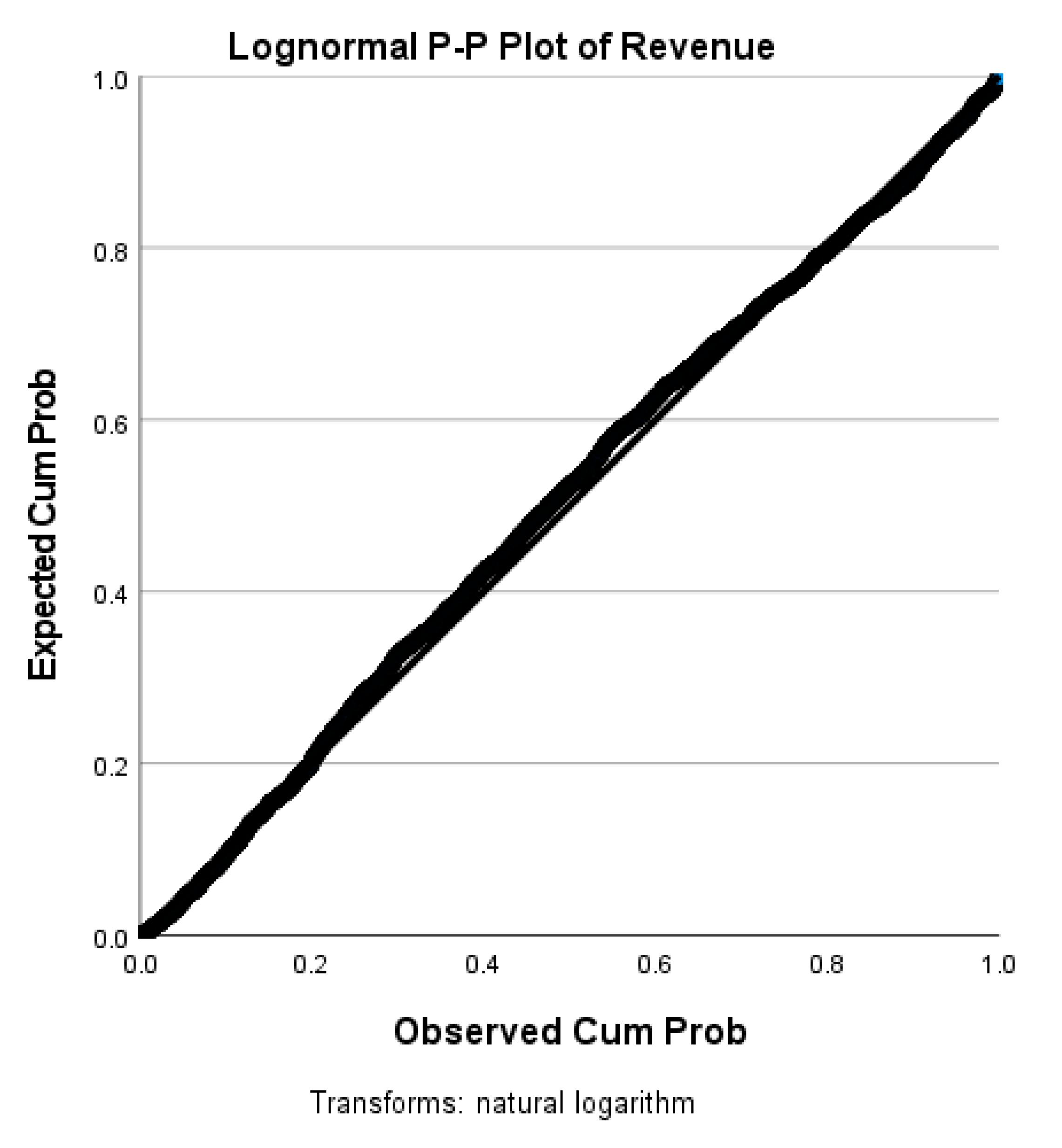
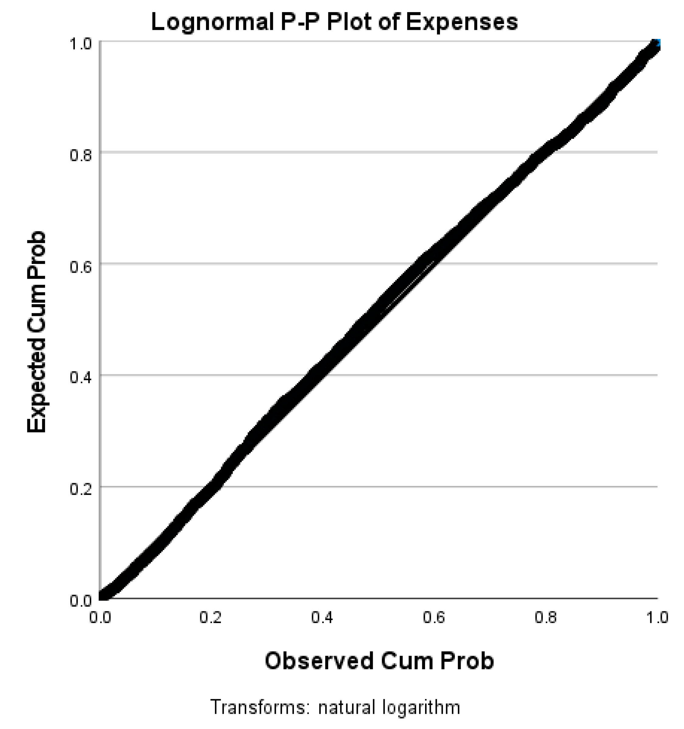
The data variables under study are the hospital’s expense and revenue from the Definitive Healthcare data for a given period of time. Our study data meets the requirement for our new method because it is not normally distributed, as is evident from the p-p plots in
Figure 1 and
Figure 2. Thus, Altman’s Z-score, Ohlson et al.’s O-score, and Hillegeist et al.’s methods are inapplicable. A new method needs to be constructed as the literature does not have a method for financial data with a lognormal normal
3.3. Software
We utilized Microsoft Mathematics 4.0 software to develop
Figure 1,
Figure 2,
Figure 3,
Figure 4,
Figure 5,
Figure 6,
Figure 7,
Figure 8 and
Figure 9.
Figure 1,
Figure 2,
Figure 10,
Figure 11,
Figure 12,
Figure 13 and
Figure 14 were generated with IBM (International Business Machines) SPSS (Statistical Package for Social Sciences) Statistics Version 28.0.1.0. The maps and tables were created with Microsoft Excel.
Stochastic Method with New Expressions
To be specific to comprehend our stochastic approach, letbe a tipping point for bankruptcy to emerge based on the levels of the revenue and expense of the hospital in a defined duration of time. First, we assumed that both revenue and expense are intricate random variables whose uncertainty is governed by a bivariate lognormal frequency structure. Second, we confirmed that our bankruptcy data follow a bivariate lognormal (BLN) frequency pattern. Because of the lognormality, the Z-score, regression. modified Altman Z-score, Ohlson O-score, and Zmijewski X-score approaches are not appropriate. The traditional regression approach is not appealing to us to analyze and interpret the data evidence for reasons such as unbalanced sampling and the existence of selection bias stated in Gruszczyński (2019).
In our new and novel stochastic approach, we developed and interpreted the theoretical regression curve to forecast the revenue given the expense level and vice versa, their correlation measure under bivariate lognormal data, risk measure for bankruptcy due to the revenue and expense , their level of information, the likelihood for a hospital’s expense to exceed the state’s median expense level, and a hospital’s financial memory level. These details are not available in the Z-score or regression approach.
The random finance variables
and
meet Lien’s reasons for considering a bivariate lognormal frequency structure in (1). The random P-P plots (see
Figure 1 and
Figure 2) below of the revenues
and the expenses
confirm that the finance variables
and
are bivariate lognormal in (1).
The joint bivariate probability frequency function (pff) of
and
in (1), with
denoting their correlation, is called lognormal:
where
are linear log transformations. The conditional pff of R for given O is
The regression curve of R on O is
Notice that when the correlation parameter vanishes (that is,
), the joint pff (1) breaks up into a product of marginal lognormal pffs
and
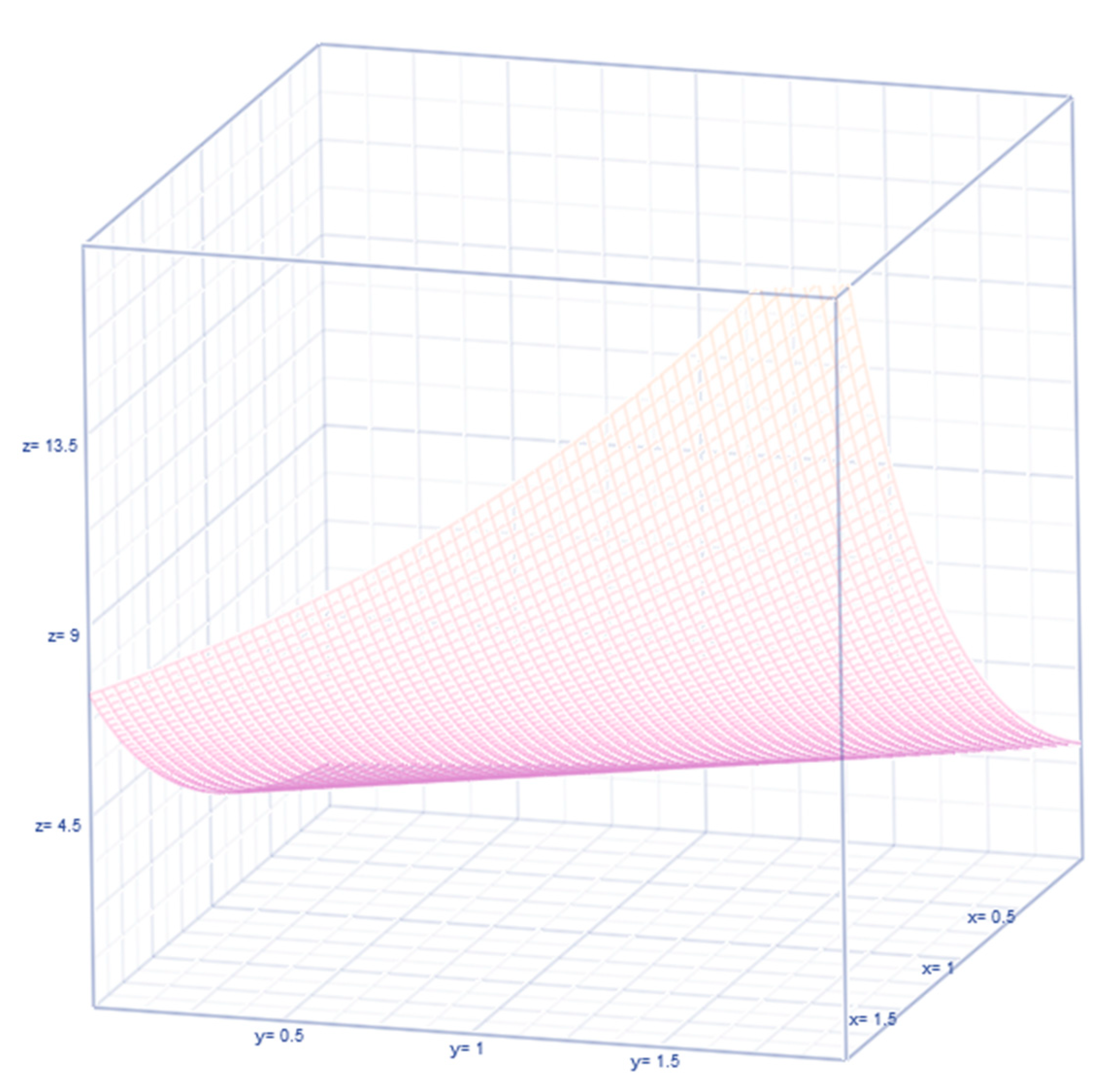
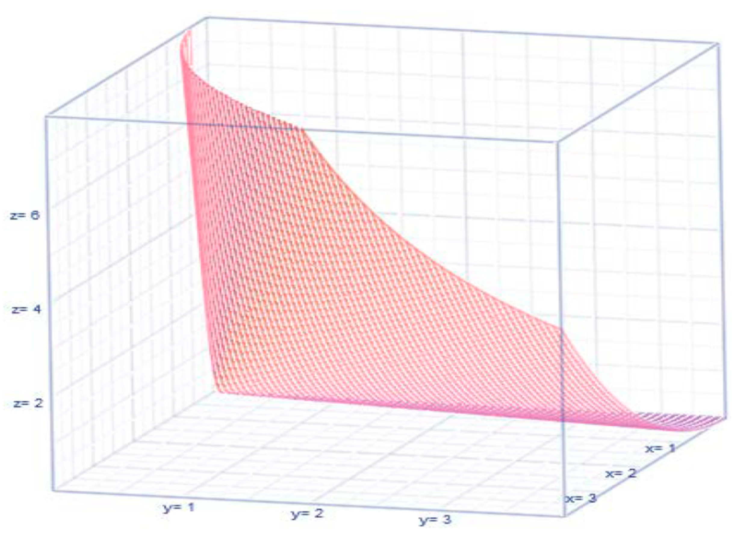
Then, the marginal baseline regressions become an exponential curve
and
(see
Figure 3), implying that neither finance variable
or
is influencing the other as a part of projecting the other.
Otherwise (that is, when the finance variables
or
are correlated), the (baseline) regressions are uplifted by a factor
or
as the case is regression to forecast
or forecast
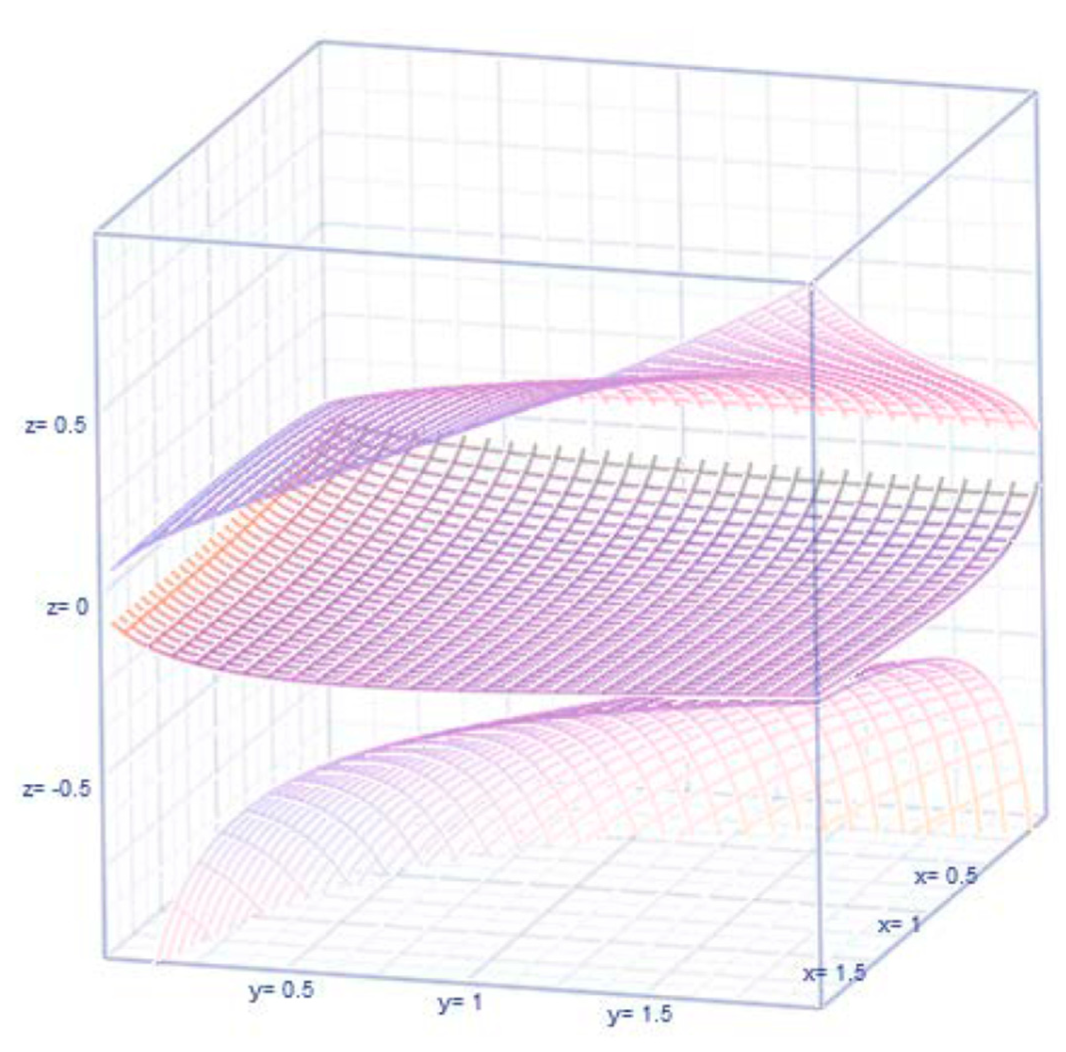
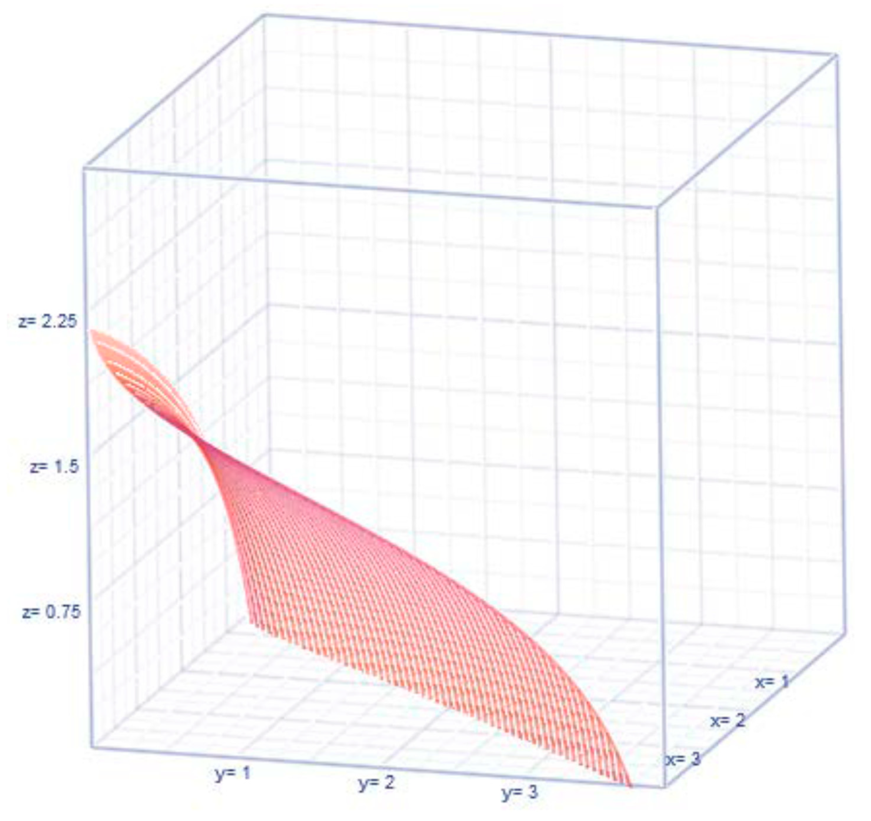
, respectively. We will compare and discuss the uplifting factors later in the article. The earliest reference to (1) is by Thoimopoulos and Longinow (1984). The expression for the correlation under the lognormal chance mechanism for the revenue and expense variables is expressed as
(see
Figure 4 for their configuration depending on the value for
).
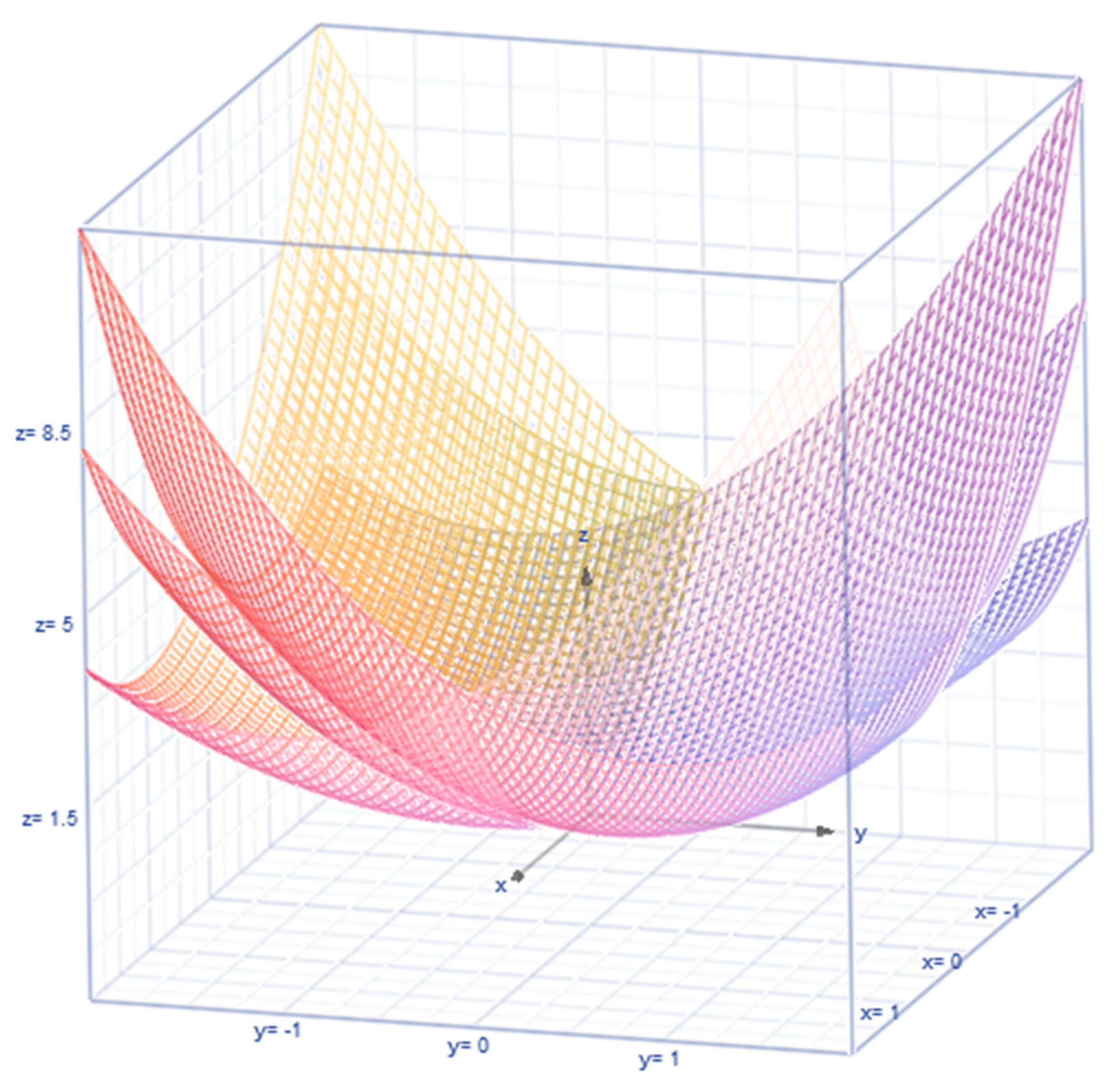
Let
,
,
,
denote respectively the marginal median and mode of the revenue, of expenses. Also, their expected values under lognormal chance mechanism for the revenue and expense variables are
,
, (see their configurations in
Figure 5) with their covariance as a function of their variances and risk
(see
Figure 6). The median and mode of the revenues and expenses are indicated by
,
,
,
.
Their entropies (which are quantified information) for the expenses and revenues are
, an
respectively. See the patterns of
or
(see
Figure 7 for their nonlinear configurations).
The above results are inadequate to capture and interpret the existence of cause or effect of bankruptcy and hence, a different version of the bivariate lognormal pff (1) needs to be modified as in the article. There are known disadvantages of using the regression approach in financial distress. In other words, the predictor (alternatively recognized as independent) variables are either incorrectly defined or insufficiently measured. The regression concept encompasses a variety of micro-techniques that are meaningful only when the assumptions are met by the data, according to Greenland (2024). The assumptions, model specifications, or interpretations are not fully understood by the regression builders. Building regressions is an art rather than a methodology to stand up for its merit. One regression fit is better than another. Yet, one regression fit cannot be declared as the best as there is a grey area. Even statisticians are not conclusively answering the right path for data analysis in building regression.
Should a Bayesian or classical (non-Bayesian) regression be resorted? Both are philosophically opposed to each other causing a dilemma in those who chose regression analysis. In the Bayesian framework, the non-observable parameter dynamically changes from one time to another, and it requires selecting judiciously prior knowledge. The classical framework is at times tedious as detailed in Nawajah et al. (2024). Another technical disadvantage exists in interpreting the regression coefficients, especially when the data of the dependent or predictor variables are transformed. The regression approach requires that the data validate the assumptions. One of the assumptions is known to be normality. Many believe that normality is a myth as it seldom exists. However, the popular regression fits are done based on the normality of the dependent variable and the constancy of the predictor variables. When the normality of the dependent variable is unmet with or without the homogeneity assumption, financial analysts are tempted to logarithmically transform the dependent variable. The profit per bed in a hospital is known to be a case in point. Such logarithmic transformation of the predictor) variable intensifies the complexity of the interpretation of the estimated regression coefficient(s). Is the interpretation useful in the defined scale of the variables? How do the finance analysts do it? Should an undoing/reversing of the transformation scale of the regression results occur? More often than otherwise, the reversing of the transformation scale would unravel a reality that the dependent and predictor variable(s) are nonlinearly interrelated before the transformation. The scale-powered transformation or for an appropriate choice is resorted at times.
Note that the finance variables
and
are correlated bivariate lognormal variables. Needless to mention that
and
are correlated bivariate normal variables with parameters
, according to Chattamvelli and Shanmugam (2022). There are two mutually exclusive possibilities in this context: The first possibility is the earliest tipping point,
in which the revenue,
is over the proportion,
times of the expenses
. The probability of the event
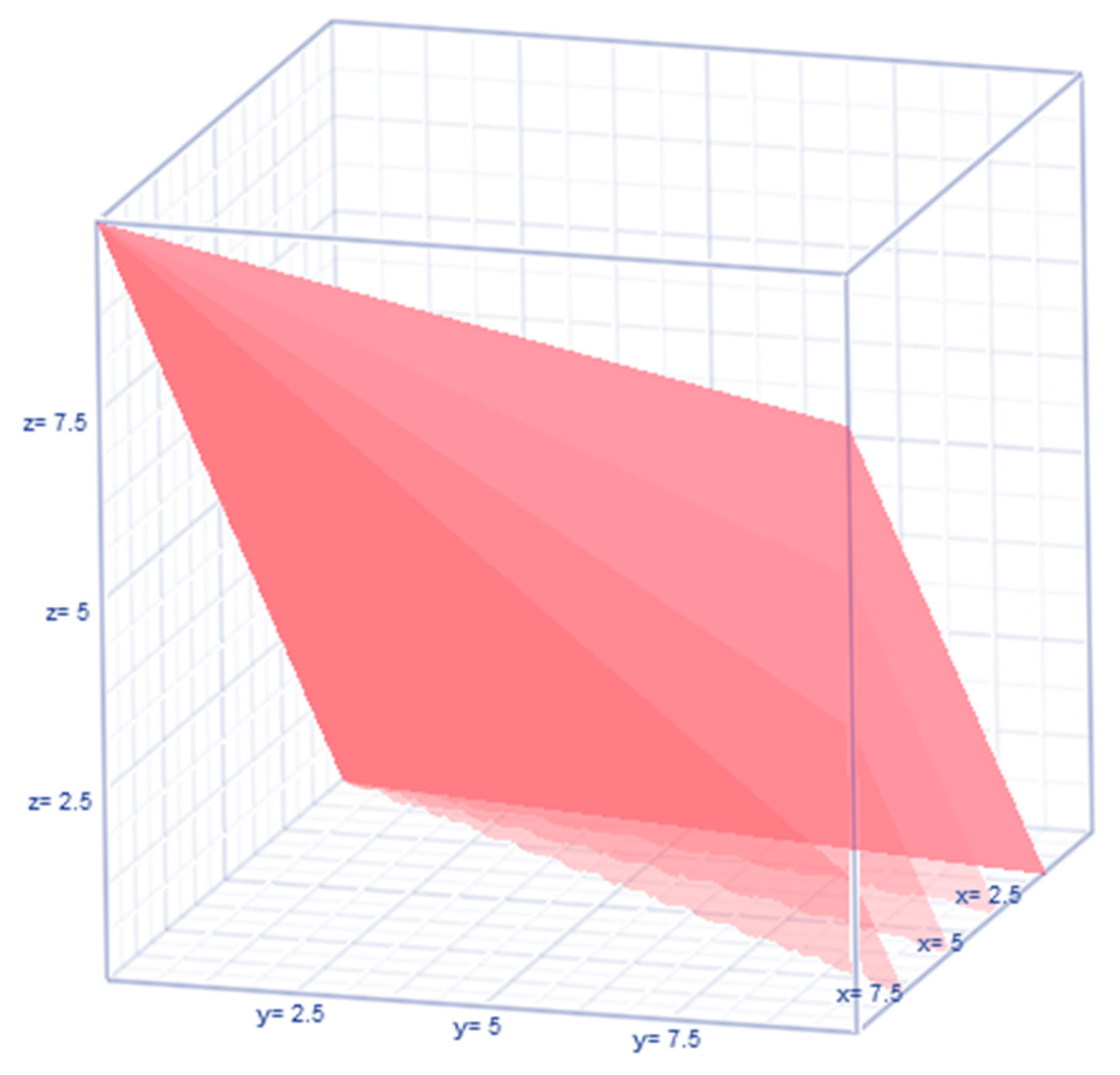
is not of any concern to the hospital and hence it is not pursued in the article. The second (complementary) mutually exclusive possibility is the event
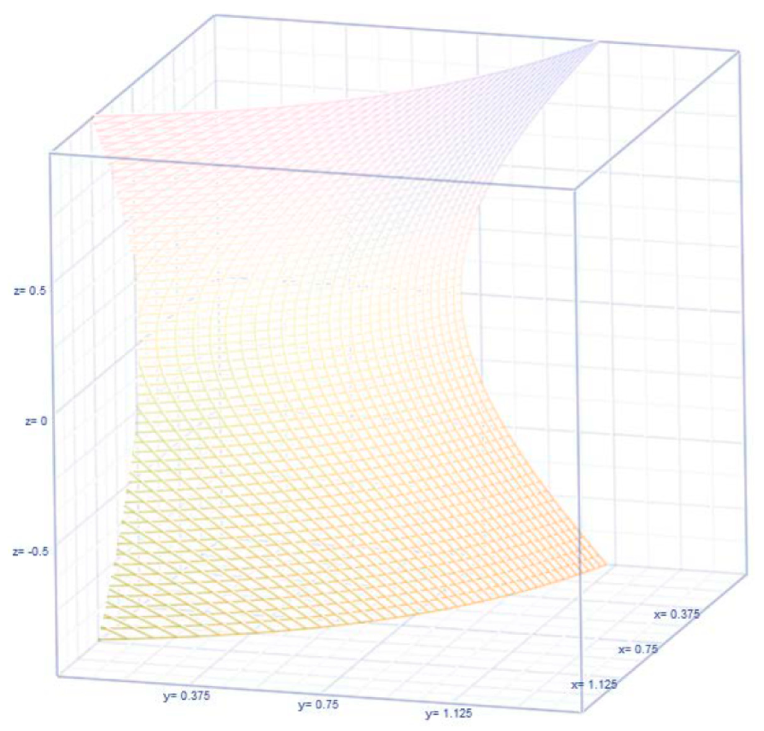
, which is indicative that the hospital moves into a zone in which bankruptcy might emerge. See the nonlinear dynamics of the inequality
in
Figure 8. That is,
The likelihood for the revenue,
is lesser than a proportion,
of the expenses,
could be cast in probability terms as in
. Using the conditional pff (2) and the marginal pff (4), we rewrite
, where
is the cumulative normal frequency structure. We now Taylorize
at the tipping point
. That is
. The derivative of the integral is further simplified to
using the formula in (Blumenfeld, 2001, page 198). Going back to the expression for
, we seek its closed form expression as in (6) for the sake of computing the probability. For this purpose, the probabilistic risk for the revenues to be less than the expenses is needed. Realize that such a risk is a function of the tipping point
, mean
and variance
of the expenses
, and their correlation parameter
. That is,
When the revenues
and the expenses
are close to each other, the tipping point is
. In which case, the probability in (6) is
. The expression (6) is indicative of the risk of financial stress emerging in the sense that the revenue is lower than the expenses, which is a prelude for bankruptcy i as a possible outcome. Realize that the chance for the revenue to be lesser than the expenses in (6), only the tipping point
, the correlation
between the revenue and expenses, and the average and variance of the expenses are involved. Hence, we need to capture the patterns of the expenses
. In the literature (see Chattemvelli and Shanmugam, 2022), the local dependence of the revenue and expenses with a bivariate normal frequency pattern is echoed by
. However, in the alternate situation in which the revenues and expenses of a hospital’s system are governed by a bivariate lognormal frequency pattern, their dependence changes to
. Furthermore, the likelihood for the expenses to exceed the state’s median expense level
is
with the bankruptcy incidence rate
. Notice also that when the survival chance S(t) for the expenses to exceed a tolerance level is slimmer, the bankruptcy incidence rate i(t) is more frequent. In a probabilistic sense, the frequency of the incidence rate to bankruptcy is connected to the hospital’s financial memory. This article now derives an analytic expression to capture and interpret the hospital’s financial memory as in (8). Notice the expression (8) for the hospital’s financial memory is controlled by the mean µ
O, volatility σ
O of the hospital’s expenses. The mean excessive frequency pattern of the expenses exceeding the tolerance level
is
, where the memory of the hospital’s finance system plays a role. The memory of the hospital’s expenses pattern is
In any situation (not necessarily only in the bankruptcy) situation, under the bivariate lognormal frequency pattern of the expenses and revenues, their variances are known to be non-ignorable. Issa et al. (2024) defined the financial risk in terms of the variances and covariances of the finance variables. In the bankruptcy context, the variation of the expenses and revenues is built in an elliptical orbit
as shown in
Figure 9.
4. Results
The expense variable
and the revenue variable
in the data are correlated at a level
, with a 95% confidence interval
. See the value of the Probability Prob (
<
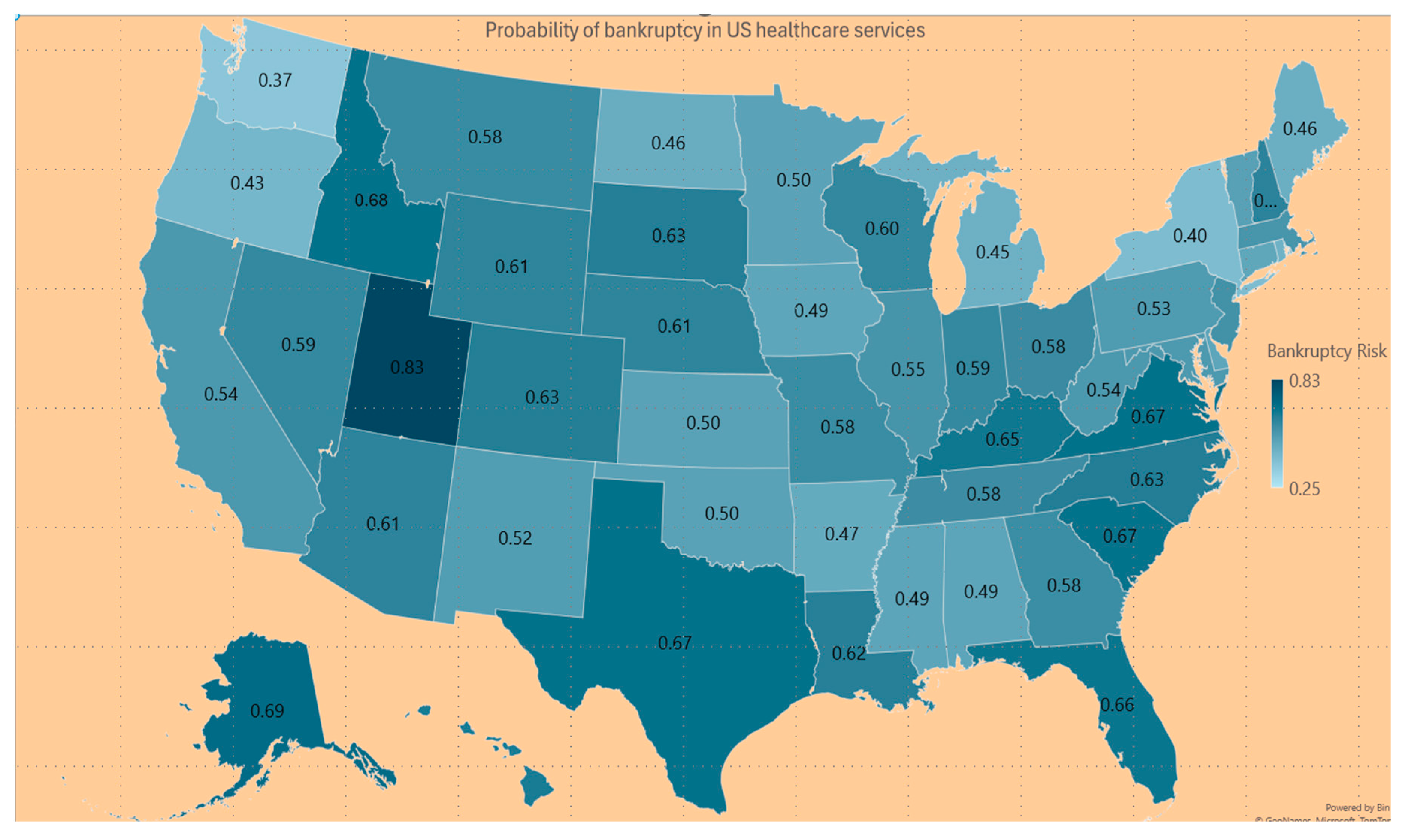
) of the expression (6) in Column 1 of
Table 1, and
Figure 10 for the US hospitals to probability to become bankrupt. See in Column 2 of
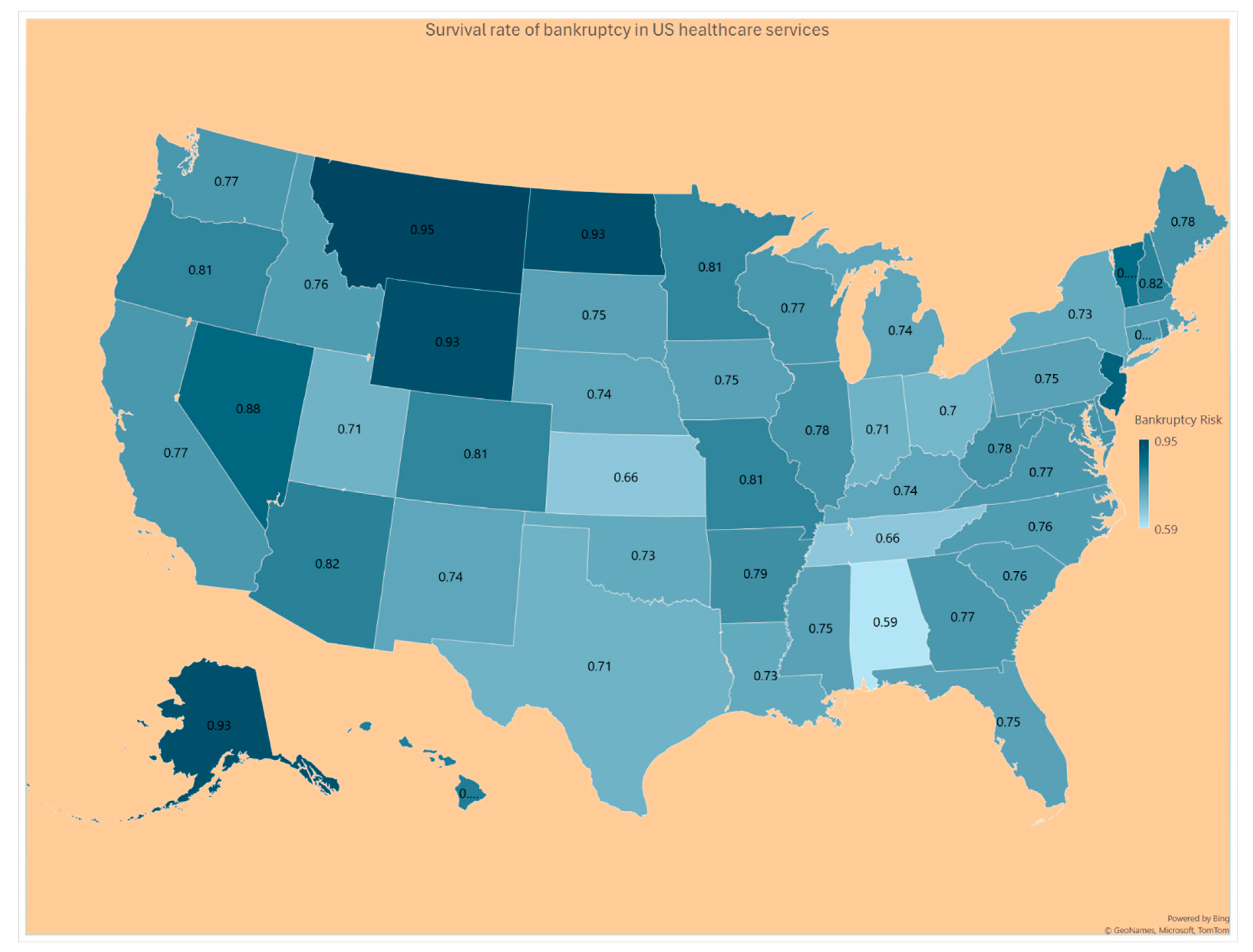
Table 1 and
Figure 11, the Survival rate S(t) = Pr (
> t) for a hospital’s expenses to exceed a given tolerance level t. Because the average and variances of the hospital’s expenses are extremely large numbers, the probability for the excessive expenses to exceed the tolerance level
(that is,
) is near zero and hence, their values are not displayed in
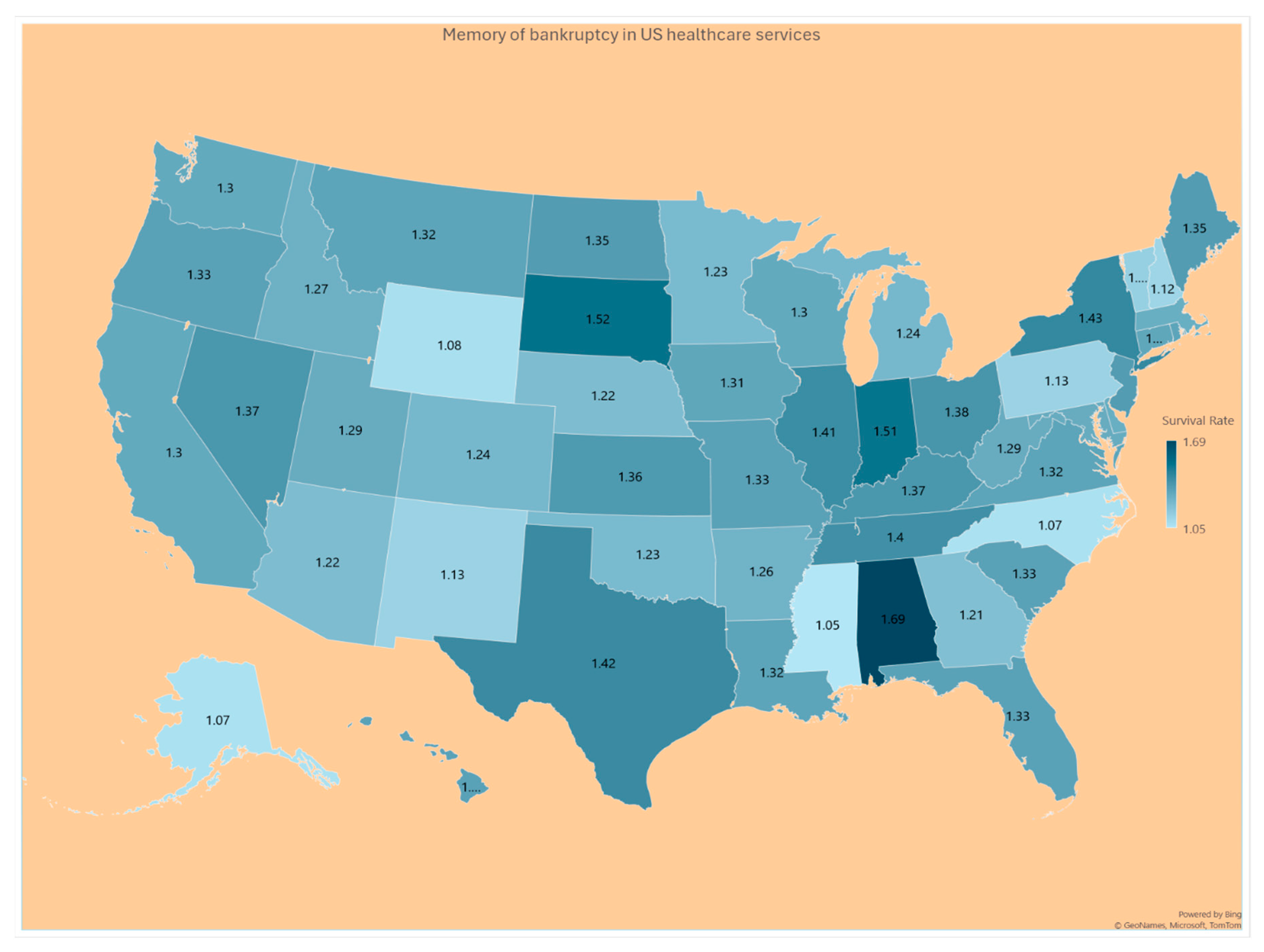
Table 1. However, the hospital’s memory to hold on to the patterns of finance variables in expression (8) is displayed in the 3
rd Column of
Table 1 as the memory is finite around the baseline value 1.0 across the US states as seen in
Figure 12.
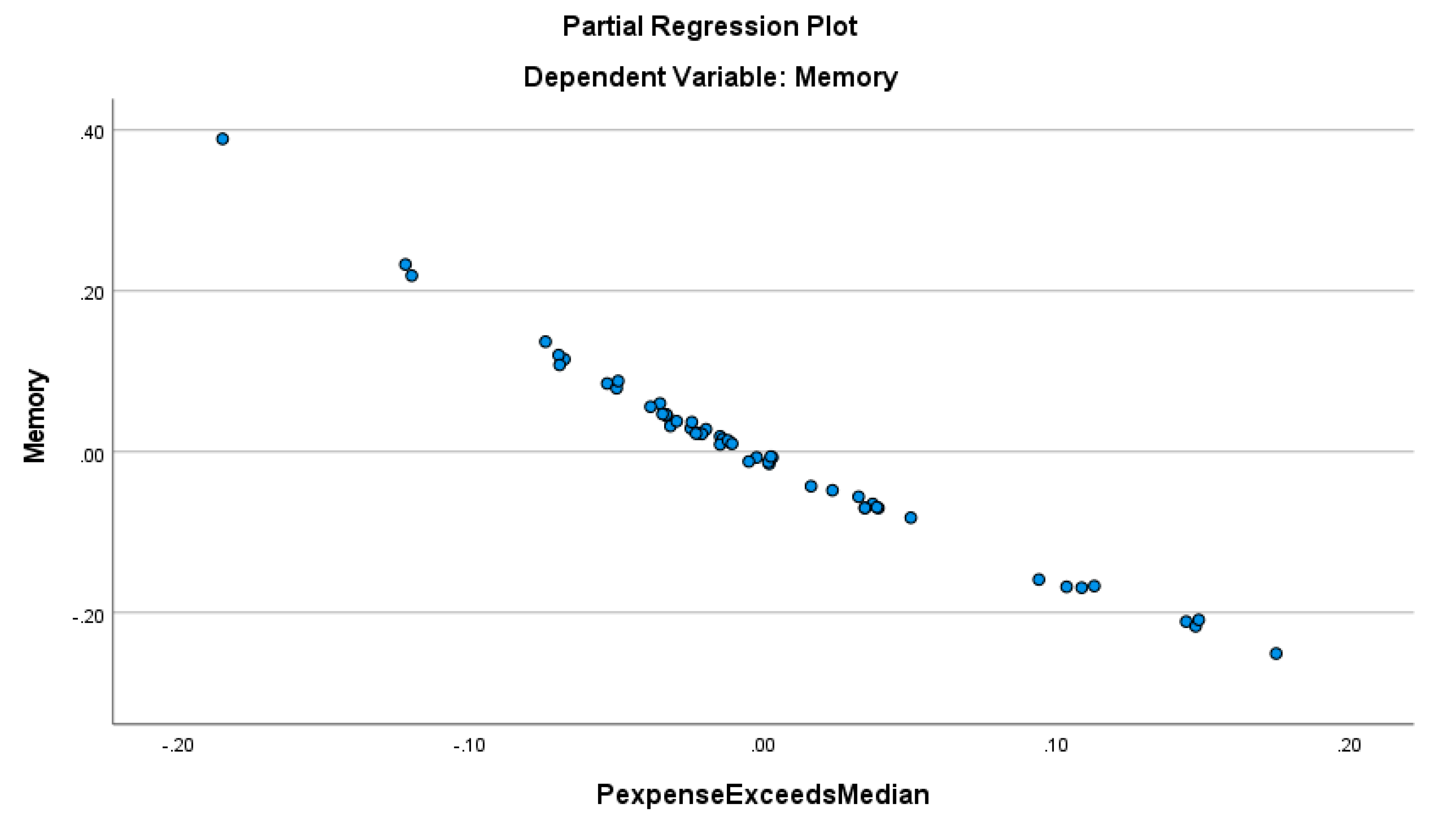
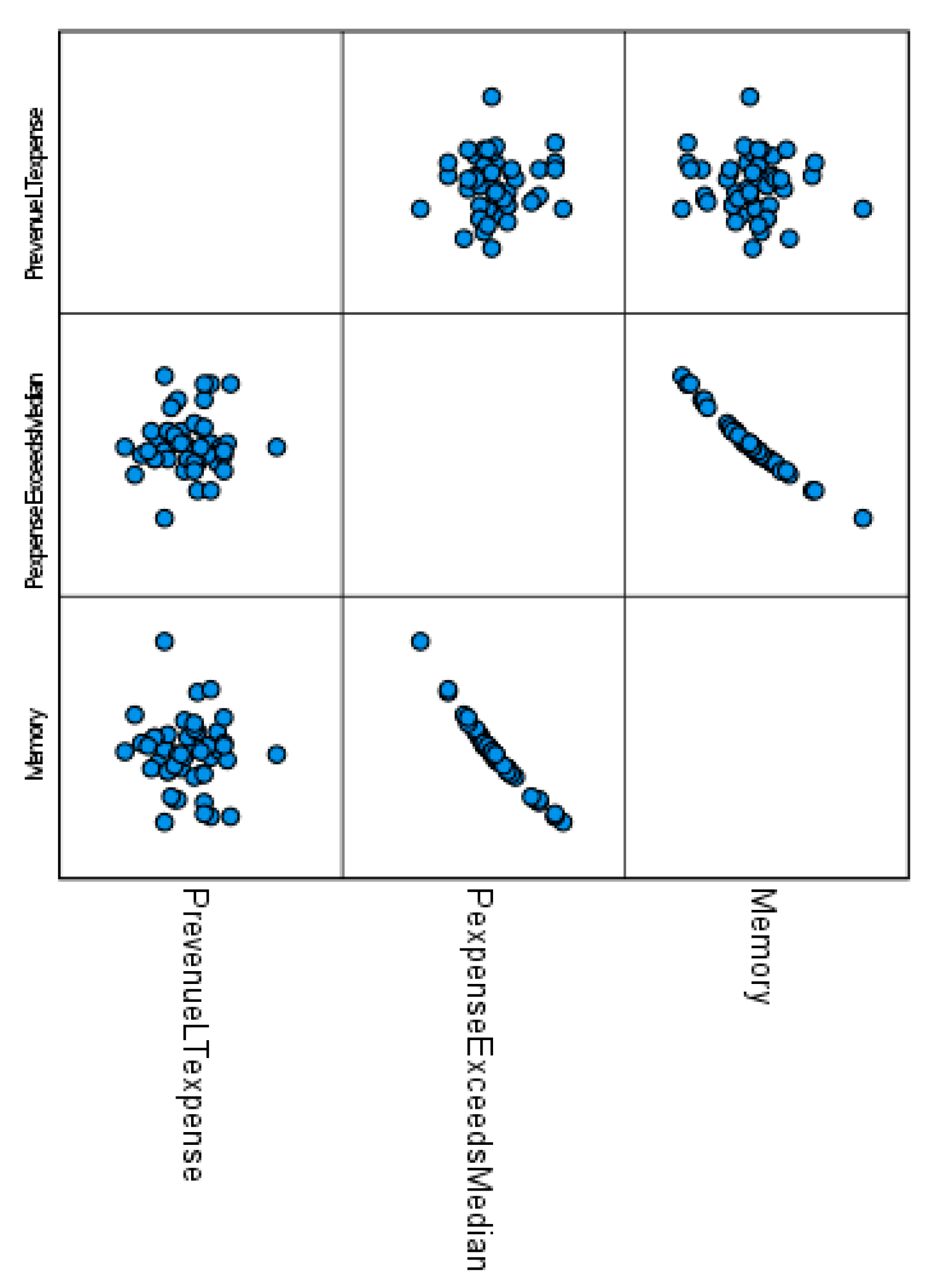
Figure 13 suggests that the memory level of the hospitals’ financial system is less only when the probability for the expenses to exceed the state’s median expense is higher. In other words, the hospitals’ financial system is more predictable by the proportion of the hospitals spending more than the state’s median expense, with an R-squared higher than 0.975. The proportion of the hospitals with revenue less than the expenses is not a significant predictor of the memory of the hospitals’ financial system, as confirmed by the correlograms in
Figure 14.
Figure 14 provides the correlation pattern among all three analytic results (namely Pr (Revenue < Expenses), Pr (Expenses exceeds the State’s Median Expense), and the hospital’s memory of the finance variables) across the US states which reveals an interesting advantage of our stochastic approach as these are not possible in the Z-score, regression, modified Altman Z-score, Ohlson O-score, or Zmijewski X-score approach.
5. Discussion
This study aimed to provide a new method for analyzing nonnormal financial data, and to illustrate our new method by analyzing a US acute care hospital financial bankruptcy dataset. The existing methods to analyze financial variables for the sake of warning the likelihood of forthcoming bankruptcy require the frequency pattern of the data to be normal (that is Gaussian). Unfortunately, the literature has not addressed any remedy to apply in case the requirement is not met. A reason might have been that financial analysts have not been aware of the developments in probability or statistical theory. The statistics community might not have paid enough research attention to the needs of the financial analysts. The authors of this article have overlapping research interests between finance and statistical theory.
Our results indicated the study hospital’s expenses and revenues are significantly positively correlated, implying that more revenues might lead to more expenses, which is quite expected. The stress in the administration of the hospitals is an issue when the expenses exceed the revenue, and it is in essence the root cause of bankruptcy. The memory level of the hospital’s uncertainty system is the opposite of what we desire. When the hospital’s expense exceeds the state’s average expense, the memory level ought to be higher to safeguard from being trapped in the possibility of bankruptcy but it did not happen so unfortunately. There must have been reasons residing in the financial variables. Such reasons might include urban versus rural locations, poor local economy, too much inflowing migration of the population, unhealthy conditions of the states, etc. A few examples that are vulnerable to bankruptcy are Utah, Michigan, Florida, and Texas. Most of the coastal states in the eastern or western US are less likely to be drawn into bankruptcy. More intensive research is needed to track the important reasons why hospitals in Washington, Oregon, Louisiana, Mississippi, New York, North Dakota, and Arkansas are less likely to experience bankruptcies when their chance of making less revenue than the expenses is less than 50%.
There has been a tendency in almost all US states for a hospital to outspend more than the average expense of the state and it is so in the thinly populated states like Hawaii, Montano, Wyoming, and North Dakota. In almost all US states, the memory of excessive spending over the state’s average expense is higher than the baseline memory 1.0 except in states of Hawaii, Wyoming, Virginia, North Carolina, Mississippi, and Arkansas. When such a hospital’s memory is greater than 1.0, there might be conscious efforts to prevent bankruptcy from occurring. In our stochastic approach, the concept of memory personifies conscious or unconscious efforts by the hospital administrators’ reaction to the continuing pattern in which the hospital’s revenue has been lesser than the expenses. The higher level of such memory level is indicative of a lower chance for bankruptcy to occur. Our stochastic approach helps to identify such US states in the topic of providing indications for the likelihood of US hospital bankruptcies.
5.1. Limitations and Future Research
This study has some limitations. First, we analyzed Definitive healthcare data for the calendar year 2022, with lagged independent and control variables from 2021 to mitigate endogeneity and reverse causality. Future research drawn from a longitudinal dataset could reveal new insights into the probability of hospital bankruptcy.
Second, future research could examine our studied relationship at a more granular level. Such work might consider looking at the likelihood of bankruptcy at the county level. Coupled with the sort of mapping that we endeavored to provide in our paper, such work may provide healthcare policy makers with a clearer understanding of what areas of the state, region, or country may be the most at risk and in need of financial assistance or intervention.
Third, there could be other factors affecting bankruptcy that were not accounted for in our study. Future studies should consider adding more organizational and market variables which may reveal new factors related to predicting hospital bankruptcies. For example, higher labor expense ratios vis-à-vis local competitors or the use of contract labor can significantly reduce a hospital’s profit margin. Beauvais et al. (2023), found numerous other factors reduce the likelihood of bankruptcy including Joint Commission accreditation, Hospital Consumer Assessment of Health Care Providers and Systems (HCAHPS) survey results, higher liquidity ratios, less competitive markets, increased Medicare payer mix, and a higher case mix index. Several other factors increased the likelihood of bankruptcy in their study, including facility age, higher Medicaid payer mix, and the hospital’s serious complication rate.
6. Conclusions
The analytic expressions of this article are appropriate for an analysis of financial variables such as revenue and expenses only if their data display a bivariate lognormal frequency pattern. Other financial variables could be analyzed if their data follow a bivariate frequency pattern. It is worth pointing out here that the finance variables could follow a frequency pattern other than the lognormal frequency pattern. In such scenarios, the concept of stochastic approach could be retained but new appropriate expressions for the specific bivariate frequency pattern need to be devised.
Author Contributions
All authors contributed equally to Conceptualization, methodology, software, formal analysis, resources, data curation, writing, and visualization. All authors have read and agreed to the published version of the manuscript.
Informed Consent Statement
Not applicable.
Data Availability Statement
Acknowledgments
We acknowledge and thank Cristian Lieneck, Director of the School of Health Administration, for his encouragement.
Conflicts of Interest
None.
References
- Aitchison, J., Brown, J., 1957. Lognormal Frequency structure: With Special Reference to its Uses in Economics. Cambridge University Press.
- Altman, E. I. (2018). Applications of distress prediction models: what have we learned after 50 years from the Z-score models?. International Journal of Financial Studies, 6(3), 70.
- Altman, E.I. Financial ratios, discriminant analysis and the prediction of corporate bankruptcy. J. Finance. 1968, 23, 589–609.
- Beauvais, B., Ramamonjiarivelo, Z., Betancourt, J., Cruz, J., & Fulton, L. (2023, January). The Predictive Factors of Hospital Bankruptcy—An Exploratory Study. In Healthcare, Vol. 11, No. 2, p. 165-183.
- Definitive, (2024). https://www.ncbi.nlm.nih.gov/pmc/articles/PMC9858769/.
- Microsoft Mathematics-4. https://microsoft.com/microsoft-mathematics-4.
- Bellovary, J.L.; Giacomino, D.E.; Akers, M.D. (2007). A review of bankruptcy prediction studies: 1930 to present. J. Finance. Educ., 33, 1–42.
- Blumenfeld, D. (2001). Operations research calculations handbook. CRC press.
- Chattamvelli, R., & Shanmugam, R. (2022). Continuous Distributions in Engineering and the Applied Sciences--Part I. Springer Nature.
- Citterio, A. (2024). Bank failure prediction models: Review and outlook. Socio-Economic Planning Sciences, 101818.
- Dobkin, C., Finkelstein, A., Kluender, R., & Notowidigdo, M. J. (2018). The economic consequences of hospital admissions. American Economic Review, 108(2), 308-352. [CrossRef]
- Dubas-Jakóbczyk, K., Ndayishimiye, C., Szetela, P., & Sowada, C. (2024). Hospitals’ financial performance across European countries: a scoping review protocol. BMJ open, 14(1), e077880.
- Gomes, C., Campos, F., Malheiros, C., & Lima Santos, L. (2023). Restaurants’ Solvency in Portugal during COVID-19. International Journal of Financial Studies, 11(2), 63.
- Greenland, S. (2024). Regression methods for epidemiological analysis. In Handbook of epidemiology (pp. 1-76). New York, NY: Springer New York.
- Gruszczyński, M. (2019). On unbalanced sampling in bankruptcy prediction. International Journal of Financial Studies, 7(2), 28. [CrossRef]
- Hillegeist, S. A., Keating, E. K., Cram, D. P., & Lundstedt, K. G. (2004). Assessing the probability of bankruptcy. Review of accounting studies, 9, 5-34. [CrossRef]
- Issa, S., Bizel, G., Jagannathan, S. K., & Gollapalli, S. S. C. (2024). A Comprehensive Approach to Bankruptcy Risk Evaluation in the Financial Industry. Journal of Risk and Financial Management, 17(1), 41. [CrossRef]
- Ivanova, M. N., Nilsson, H., & Tylaite, M. (2024). Yesterday is history, tomorrow is a mystery: Directors’ and CEOs’ prior bankruptcy experiences and the financial risk of their current firms. Journal of Business Finance & Accounting, 51(1-2), 595-630. [CrossRef]
- Koptseva, E. P., Paristova, L. P., & Sycheva, E. G. (2022). Model for determining the probability of airline bankruptcy. Transportation Research Procedia, 61, 164-170.
- Kyoud, A., El Msiyah, C., & Madkour, J. (2023). Modelling systemic risk in Morocco’s banking system. International Journal of Financial Studies, 11(2), 70. [CrossRef]
- Letkovský, S., Jenčová, S., & Vašaničová, P. (2024). Is Artificial Intelligence Really More Accurate in Predicting Bankruptcy? International Journal of Financial Studies, 12(1), 8. [CrossRef]
- Li, X. (2024, February). Comparing Linear Regression and Decision Trees for Housing Price Prediction. In 2023 International Conference on Data Science, Advanced Algorithm, and Intelligent Computing (DAI 2023) (pp. 77-84). Atlantis Press.
- Lien, D. (2005). On the minimum and maximum of bivariate lognormal random variables. Extremes, 8, 79-83.
- Lien, D. H. D. (1986). Moments of ordered bivariate log-normal frequency structures. Economics Letters, 20(1), 45-47.
- Muñoz-Izquierdo, N., Camacho-Miñano, M. D. M., Segovia-Vargas, M. J., & Pascual-Ezama, D. (2019). Is the external audit report useful for bankruptcy prediction? Evidence using artificial intelligence. International Journal of Financial Studies, 7(2), 20.
- Nawajah, I., Kanj, H., Kotb, Y., Hoxha, J., Alakkoumi, M., & Jebreen, K. (2024). Bayesian regression analysis using median rank set sampling. European Journal of Pure and Applied Mathematics, 17(1), 180-200.
- Ohlson, J.A. Financial ratios and the probabilistic prediction of bankruptcy. J. Account. Res. 1980, 18, 109–131.
- Beauvais, B., Ramamonjiarivelo, Z., Betancourt, J., Cruz, J., & Fulton, L. (2023, January). The Predictive Factors of Hospital Bankruptcy—An Exploratory Study. In Healthcare (Vol. 11, No. 2, p. 165). MDPI.
- Phan, L. N., Beruvides, M. G., & Tercero-Gómez, V. G. (2024). Statistical Analysis of Minsky’s Financial Instability Hypothesis for the 1945–2023 Era. Journal of Risk and Financial Management, 17(1), 32.
- Prusak, B. (2018). Review of research into enterprise bankruptcy prediction in selected central and eastern European countries. International Journal of Financial Studies, 6(3), 60.
- Rastogi, S. (2024). Rural Health Care in the Age of Hospital Bankruptcies. Emory Bankruptcy Developments Journal, 40(2), 215.
- Ratnasari, I., Nugraha, N., & Sutardiyanta, I. (2024). Predicting Bankruptcy of Pharmaceutical Companies Using the Altman Z-Score and Grover Methods. Accounthink: Journal of Accounting and Finance, 9(1).
- Santoso, N. W., Kusumawardhani, R., & Maulida, A. (2024). Comparative Analysis of The Altman, Ohlson, And Zmijewski Models to Predict Financial Distress During the Covid-19 Pandemic. MAKSIMUM: Media Akuntansi Universitas Muhammadiyah Semarang, 14(1), 13-21.
- Shi, Y., & Li, X. (2021). Determinants of financial distress in the European air transport industry: The moderating effect of being a flag-carrier. Plos One, 16(11), e0259149.
- IBM SPSS Statistics for Windows, Version 28.0 (Computer Software); IBM Corp; Armonk, NY, USA.
- Thoimopoulos, N. T., & Longinow, A. (1984). Bivariate Lognormal Probability Frequency structure. Journal of Structural Engineering, 110(12), 3045-3049.
- van Dijk, T. S., Felder, M., Janssen, R. T. J. M., & van der Scheer, W. K. (2023). For better or worse: Governing healthcare organizations in times of financial distress. Sociology of Health & Illness, 1–22. [CrossRef]
- Wieczorek-Kosmala, M. (2021). COVID-19 impact on the hospitality industry: Exploratory study of financial-slack-driven risk preparedness. International Journal of Hospitality Management, 94, 102799.
- Xu, Y., Kou, G., Peng, Y., Ding, K., Ergu, D., & Alotaibi, F. S. (2024). Profit-and risk-driven credit scoring under parameter uncertainty: A multiobjective approach. Omega, 125, 103004.
- Zmijewski ME (1984) Methodological Issues Related to the Estimation of Financial Distress Prediction Models. J Account Res 22:59–82. [CrossRef]
|
Disclaimer/Publisher’s Note: The statements, opinions and data contained in all publications are solely those of the individual author(s) and contributor(s) and not of MDPI and/or the editor(s). MDPI and/or the editor(s) disclaim responsibility for any injury to people or property resulting from any ideas, methods, instructions or products referred to in the content. |
© 2024 by the authors. Licensee MDPI, Basel, Switzerland. This article is an open access article distributed under the terms and conditions of the Creative Commons Attribution (CC BY) license (http://creativecommons.org/licenses/by/4.0/).
