Preprint
Article

A Homogeneous Gravitational Collapse Model With Λ Parametrization

Altmetrics

Downloads

90

Views

27

Comments

0

This version is not peer-reviewed

Submitted:

03 July 2024

Posted:

04 July 2024

You are already at the latest version

Alerts
Abstract
The present work deals with the study of the gravitational collapsing phenomenon of spherically symmetric massive stars with a Λ parameterization A collapsing model with a cosmological constant of the form Λ=β(θ ̇/3+θ^2/9) has been considered. In this model, exact solutions of the Einstein field equations (EFEs) are obtained using the $\Lambda$ parametrization and the junction conditions. All the physical and geometrical quantities are calculated in terms of the Schwarzschild mass M and areal radius R of spherically symmetric stars. Consequently, we have approximated the masses and radii of different stars to estimate the value of the model parameter β. We discuss the collapsing process and singularity formation for these stars and observe that all the physical and geometrical parameters of the model heavily depend on the model parameter β. We further discuss spacetime singularity through the development of apparent horizons.
Keywords: 
Subject: Computer Science and Mathematics  -   Applied Mathematics

1. Introduction

Gravitational collapse is a phenomenon in astrophysics where a massive object, such as a star, undergoes a rapid and intense contraction due to the force of gravity overcoming internal pressure. This phenomenon is a fundamental aspect of astrophysics and plays a crucial role in the formation and evolution of celestial bodies. Gravitational collapse occurs when an astronomical object is unable to counteract the pull of its own gravity. White dwarfs and neutron stars often develop as a result of collapse processes. When the internal pressure of the star balances the pull of its own gravity during thermonuclear burning, the star is in an equilibrium configuration. As a result, after the nuclear burning is complete, the star may, depending on its mass, once again have an equilibrium configuration as a neutron star or white dwarf. Also, in general relativistic gravitational collapse, one should match the interior and exterior geometry of the collapsing object through the proper junction condition. The problem of general relativistic gravitational collapse has attracted attention from researchers since the development of Einstein’s theory of general relativity in the early 20th century. Gravitational collapse has gained prominence as a natural extension of general relativity and its implications for extreme astrophysical scenarios. The initial interest in the general relativistic gravitational collapse problem was developed with the pioneering landmark paper by J. Robert Oppenheimer and Hartland Snyder in 1939 [1]. They applied general relativity to the collapse of massive stars and predicted the formation of black holes. The discovery of solutions like the Kerr metric (describing the rotating black holes) and the formulation of black hole thermodynamics by Stephen Hawking and Roger Penrose increased interest in the nature of black holes and their role in gravitational collapse. Roger Pnrose proposed the cosmic censorship conjucture (CCC) in the 1970s, suggesting that naked singularities are not formed through the gravitational collapse process, i.e., the space-time singularity formed by gravitational collapse should be hidden behind the horizon; this means the end state of a collapsing star must be a black hole (BH). This conjucture spurred further research into the nature of singularities and the stability of black holes. However, there is no mathematical proof in support of CCC, and various models have been published in the literature that depict the ultimate fate of the collapsing star as a naked singularity (NS). This hypothesis led to extensive research and discussion in the field, and its validity is still a topic of investigation and debate in theoretical physics. Later, Indian theoretical physicist Pankaj Joshi contributed significantly to the study of gravitational singularities, including the concept of the naked singularity. He explored scenarios in which gravitational collapse may lead to the formation of a naked singularity rather than a black hole. Thus, the final fate of the collapsing star is still an unresolved problem and has attracted the attention of many researchers for many years, starting with the seminal paper by Oppenheimer and Synder. Although many other gravitational theories exist and are crucial to theoretical astrophysicists, the study primarily focuses on singularity formation within the context of the general theory of relativity [2,3,4,5,6,7,8,9,10]. Astrophysical observations suggest that about 71% of the universe is composed of dark energy and 24% is composed of dark matter. The nature of dark energy as well as dark matter is unknown, and many different models, like quintessence [11,12], DGP branes [13,14], Gauss-Bonnet [15,16], dark energy in brane worlds [17,18,19,20,21,22], and cosmological constant [23] in Einstien’s field equation, are proposed to explain the nature of dark energy. The cosmological constant ( Λ ) model is one of the most important among these. The cosmological constant is the energy related to the vacuum, or empty space. Cosmology has a very interesting and remarkable history with the cosmological constant problem. It has previously been discussed many times why the non-zero cosmological constant should be included in the Einstein field equations for both theoretical and observational reasons. The results of type Ia supernovashow that the universe is accelerating rather than decelerating [20]. These findings suggest that a non-zero cosmological constant may exist in our universe. Instead of the constant Λ , the dynamical character of Λ is preferred to explain the expansion of an accelerating universe. In literature, gravitational collapse in the expanding universe is studied [21]. In a collapsing configuration, the mass of the collapsing star expands negatively, i.e., towards the core of the star. Several questions serve as the basis for our work: In what way does the cosmological constant act as a repulsive force? How does it impact the motion of a collapsing star? There are many different models that have been proposed in the literature to explain Λ ( t ) , in which natural dependence is Λ H 2 , i.e., Λ Θ 2 or Λ θ ˙ [23,24,25,26,27]. In the present work, we have considered the model Λ = β Θ ˙ 3 + Θ 2 9 , where β is a dimensionless constant parameter [27]. In our work, the motion and ultimate fate of a collapsing star are influenced by cosmological constants, and we explore whether the cosmological constant favours a collapsing model or prevents it under certain conditions. The motive of our current work is to discuss the homogeneous collapse of perfect fluid distribution and find the exact solution of Einstein’s field equation by making use of junction conditions. The paper is organised as follows: In Section 2, we have discussed the basic formalism for Einstein’s field equations and junction conditions. In Section 3, we have calculated the exact solution of Einstein’s field equations with the use of Λ parametrization. In Section 4, we discussed the dynamics of the collapsing model and estimated the model parameter β . In Section 5, we discussed the apparent horizon and singularity analysis. Section 6 contains the concluding remarks of our work.

2. Basic Formalism for the Collapsing Model

2.1. Metric and Einstien’s Field Equation

We consider the gravitational collapse of a spherically symmetric massive core of a star with finite thickness. The spacetime is divided into three distinct regions, Σ and V ± , where Σ denotes the surface of the star and V ( V + ) the interior (exterior) of the star. We assume homogeneous and isotropic FLRW spacetime inside the massive core, given as:
d s 2 = d t 2 a ( t ) 2 ( d r 2 + r 2 d Ω 2 )
where d Ω 2 d θ 2 + s i n 2 θ d ϕ and the function a depends on time coordinate ‘t’ only, a particular case of the pioneering collapsing model of Oppenheimer and Synder.
The matter inside the collapsing system is assumed to be in the form of a perfect fluid, given as
T i j = ( p + ρ ) u i u j p g i j
where p and ρ are pressure and energy density of the collapsing fluid, respectively, and the vector u i is the four velocity comoving vector satisfying u t = δ j t .
Since for collapsing configuration, the a ˙ a < 0 and collapsing rate of the star is described by the expansion scalar ( Θ )
Θ = v ; i i = 3 a ˙ a
where, dot ( . ) means the time derivative.
Let us consider Einstein’s field equations for interior space-time described by metric(1) as:
G i j = k T i j + Λ k g i j
where ( k = 8 π G c 4 ) , G i j is the Einstein tensor, T i j is the energy momentum tensor, and Λ is a cosmological constant describing the distribution of dark energy in the interior region. For systems (1) and (2), the non-vanishing components of Einstein’s field equations are
Θ 2 ˙ 3 = Λ + k ρ
Θ 2 3 + 2 3 Θ ˙ = Λ k p
The energy conservation equation (Bianchi’s identity) T j ; i i = 0 has one non-vanishing equation
3 p ρ a ˙ + ρ ˙ ρ + Θ = 0
The mass function m ( t , r ) for a spherically symmetric collapsing system that describes the total mass of the collapsing star at any instant ( t , r ) is given by [28]
m ( t , r ) = 1 2 R ( 1 + R , α R , β g α β ) = 1 2 r 3 a a ˙ 2
Kretschmann curvature ( K ) is a quadratic scalar invariant derived by full contraction of the Riemann curvature tensor and describes the geometry of a collapsing system given as: [33]
K = R i j k l R i j k l
where R i j k l denotes Riemann curvature tensor. For interior spacetime (1), we have the value of K
K = 12 a ˙ a 4 + a ¨ a 2

2.2. The Exterior Metric and the Junction Condition

Since the current work focuses on gravitational collapse in dark-energy backgrounds, the exterior region of a spherical system is thought to be the Schwarzschild-de Sitter/anti-de Sitter metric [29,30]
d s + 2 = α ( R ) d T 2 α 1 ( R ) d R 2 + R 2 d Ω 2
where α ( R ) is given by
α ( R ) = 1 2 M R ± Λ R 2 3
where the ± sign refers to the Schwarzschild de-Sitter and Schwarzschild anti de-Sitter metric, and M represents the Newtonian mass of a star (also known as Schwarzschild mass), and Λ is a cosmological constant describing the distribution of dark energy in the exterior region, where the coordinate is taken as x + i = ( T , R , θ , ϕ ) . In particular, the metric (11) reduces to the Schwarzschild spacetime for Λ = 0 . The boundary hypersurface Σ separates the interior ( d s 2 ) and the exterior ( d s + 2 ) spacetime metric. The matching of the interior metric(1) to the exterior Schwarzschild metric(11) on the hyper-surface Σ yields the junction conditions [31,32]
m ( t , r ) Σ ̲ ̲ M ± | Λ | 6 R 3
and
p D E Σ ̲ ̲ Λ
Equation (13) shows that the mass of the collapsing system is equal to the generalised Schwarzschild mass over Σ . A positive value of Λ has an additive contribution, and a negative value of Λ has a deductive contribution to the collapsing mass.
Thus, the equations (13) and (14) are the required junction conditions. [37].

3. Exact Solution of Einstien’s Field Equations: Λ Parametrization

The non-vanishing components of Einstien’s field equations (5)-(6) in the current work consist of only two independent equations, with four unknown physical parameters: a ( t ) , ρ ( t ) , p ( t ) , and Λ ( t ) . Here we have considered the variable cosmological constant Λ ( t ) . Therefore, to get the exact solution of field equations, we require two more constraints. Usually, in the general theory of relativity, we utilise the parametrization of physical and geometrical parameters to obtain the solution of EFEs. There are a number of parametrizations that have been used by many authors in the literature [23,24,25,27]. In the collapsing process of any star, the internal thermal pressure, which acts outward to the core of the star (arises due to a nuclear reaction at the core), decreases, and then the external pressure, which acts inward to the core of the star (arises due to the gravitational mass of the star), prevails over it. In collapsing configuration, a ˙ a < 0 , i.e., Θ < 0 . Since we are trying to study how Λ affects the final fate of collapsing stars, we have considered the Λ -parametrization in terms of Θ to study the collapsing configuration.There are many models that propose Λ ( t ) decay law. In order to solve field equations, we consider the Λ ( t ) term, given by [24,27]
Λ = β Θ ˙ 3 + Θ 2 9
where β is a model parameter to be determined for the masssive stars.
We assume that the matter component of a star satisfies the equation of state (EoS)
p = ω ρ
where ω ( 0 ) is a constant parameter.
By using equs.(15) and (16) into field equations (5)-(6) we get
( 1 + 3 ω ) a ˙ 2 ( t ) = ( 2 + β + β ω ) a ( t ) a ¨ ( t )
on integration it gives,
a ( t ) = c 2 t ( β 3 ) ( 1 + ω ) ( β + β ω 2 ) c 1 β + β ω 2 ( β 3 ) ( 1 + ω )
where c 1 and c 2 are arbitrary constants of integration. by using junction conditions [37] given in equs.(13) and (14) we evaluate the value of arbitrary constants c 1 and c 2 as
c 1 = t 0 ( 1 + ω ) ( β 3 ) ( β + β ω 2 ) 2 ( 3 β ) ω k Λ 0 ( β + β ω 2 ) 1 2
and
c 2 = ( 2 M ) 1 3 2 ( β + β ω 2 ) ω ( 3 β ) k Λ 0 β + β ω + 6 ω 6 ( 1 + ω ) ( β 3 ) ( β + β ω 2 ) 1 3 r 3 ( β + β ω 2 ) 4 r 0 3 ω ( β 3 ) k 1 3
using the value of c 1 and c 2 in Equation (18) we have the value of scale factor
a ( t ) = ( 2 M ) 1 3 2 ( β 3 ) ω ( β + β ω 2 ) k Λ 0 1 2 + k ( t t 0 ) ( β 3 ) ( 1 + ω ) β + β ω 2 ( 1 + ω ) ( β 3 ) 2 ( β + β ω 2 ) ω ( 3 β ) k Λ 0 β + β ω + 6 ω 6 ( 1 + ω ) ( β 3 ) ( β + β ω 2 ) 1 3 r 3 ( β + β ω 2 ) 4 r 0 3 ω ( β 3 ) k 1 3
by using Equation (21) in Equation (10) we have the value of expansion scalar Θ as
Θ = 3 k Λ 0 ( β + β ω 2 ) k Λ 0 ( t t 0 ) ( β 3 ) ( 1 + ω ) + { 2 k ( 3 β ) Λ 0 ω ( β + β ω 2 ) } 1 2
Also the value of energy density and pressure of collapsing star
ρ = 2 k ( β 3 ) Λ 0 2 ( β + β ω 2 ) { k Λ 0 ( t t 0 ) ( β 3 ) ( 1 + ω ) + { 2 k ( 3 β ) Λ 0 ω ( β + β ω 2 ) } 1 2 } 2
and
p = 2 k ( β 3 ) Λ 0 2 ω ( β + β ω 2 ) { k Λ 0 ( t t 0 ) ( β 3 ) ( 1 + ω ) + { 2 k ( 3 β ) Λ 0 ω ( β + β ω 2 ) } 1 2 } 2
Kretschmann curvature is given as
K = 12 k 4 Λ 0 4 ( β + β ω 2 ) 2 ( 5 + 6 ω + 9 ω 2 4 β ( 1 + ω ) + β 2 ( 1 + ω ) 2 ) { k Λ 0 ( t t 0 ) ( β 3 ) ( 1 + ω ) + { 2 k ( 3 β ) Λ 0 ω ( β + β ω 2 ) } 1 2 } 4
Since, from equs.(18)-(25) it can be seen that all the physical and geometrical quantities are obtained in terms of the mass of the star (M). Therefore, we obtain the solution of EFE for particular masses and radii of stars. By estimating the model parameter β , one can discuss the dynamics of a collapsing system.

4. Dynamics of Collapsing Model: Blackhole Formation

4.1. ω = 1 (Stiff Matter)

In general theory of relativity `Stiff matter’ is described by the relation p = ρ where p is fluid’s pressure and ρ is its total energy density. It can also be described by a massless scalar field. For understanding of this perfect fluid one has to examine the variation of energy density with scale factor a ( t ) . In this case energy density is propotional to 1 a 6 whereas, in the case of radiative perfect fluid the energy density is propotional to 1 a 4 . These findings suggest that our universe may have gone through a period where stiff matter dominated instead of radiation fluid. Due to that importance many researchers had considered the presence of stiff matter in FRW cosmological models and its importance is first recognized by Zeldovich [35]. Now in our model we consider the case of stiff matter ( ω =1) [24,36] and get the value of scale factor, energy density and other physical/geometrical parameters as:
a ( t ) = ( 2 M ) 1 3 2 ( β 3 ) ( β 1 ) k Λ 0 1 2 + 2 k ( t t 0 ) ( β 3 ) β 1 ( β 3 ) 4 ( β 1 ) ( 3 β ) k Λ 0 β + 3 6 ( β 3 ) 2 1 3 ( β 1 ) 1 3 2 r 3 ( β 1 ) 4 r 0 3 ( β 3 ) k 1 3
Θ = 6 k Λ 0 ( β 1 ) 2 k Λ 0 ( t t 0 ) ( β 3 ) + { 4 k ( 3 β ) Λ 0 ( β 1 ) } 1 2
p = ρ = 2 k ( β 3 ) Λ 0 2 ( β 1 ) { k Λ 0 ( t t 0 ) ( β 3 ) + { k ( 3 β ) Λ 0 ( β 1 ) } 1 2 } 2
K = 3 k 4 Λ 0 4 ( β 1 ) 2 ( 20 8 β + 4 β 2 ) { k Λ 0 ( t t 0 ) ( β 3 ) + { k ( 3 β ) Λ 0 ( β 1 ) } 1 2 } 4
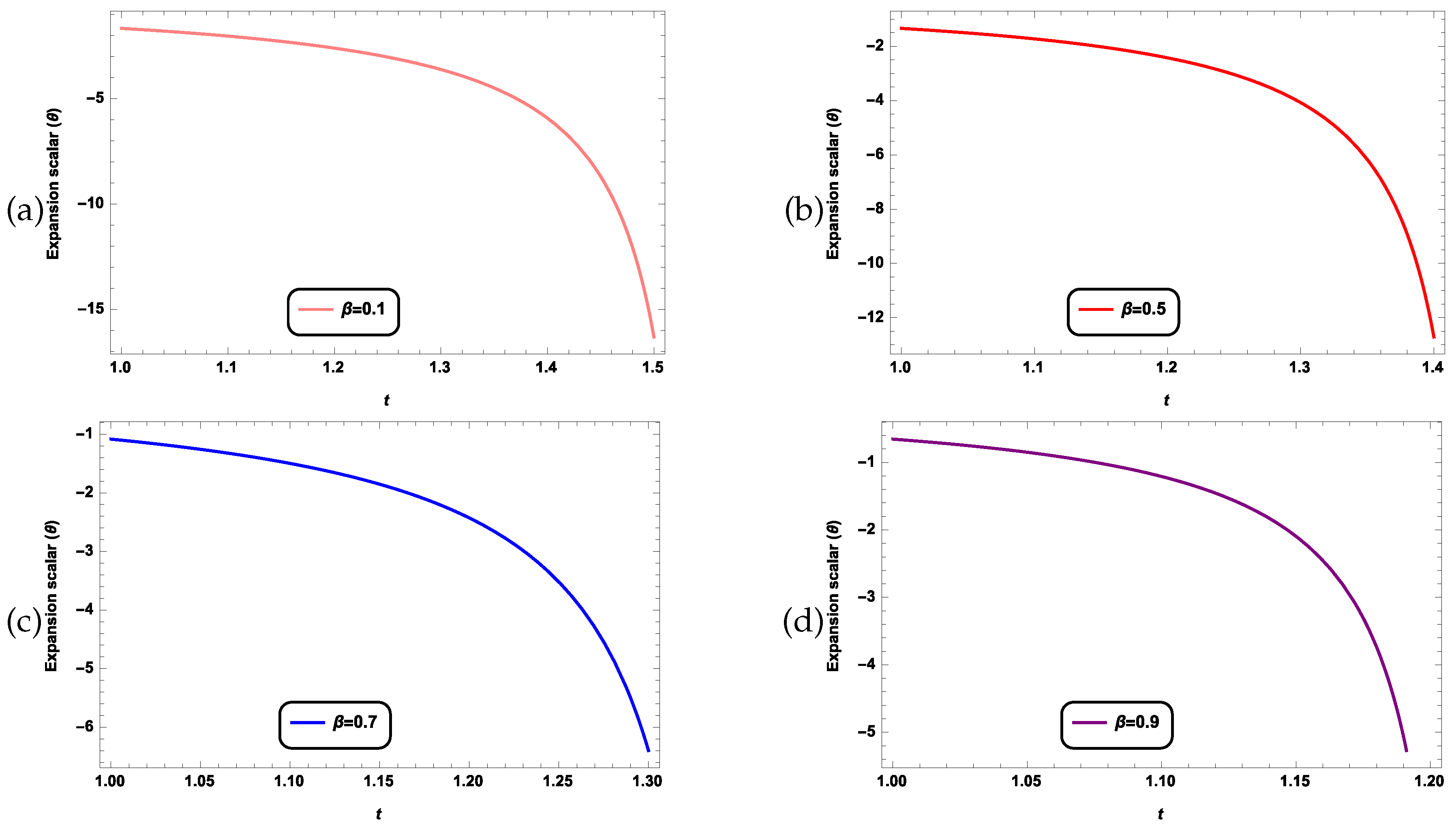
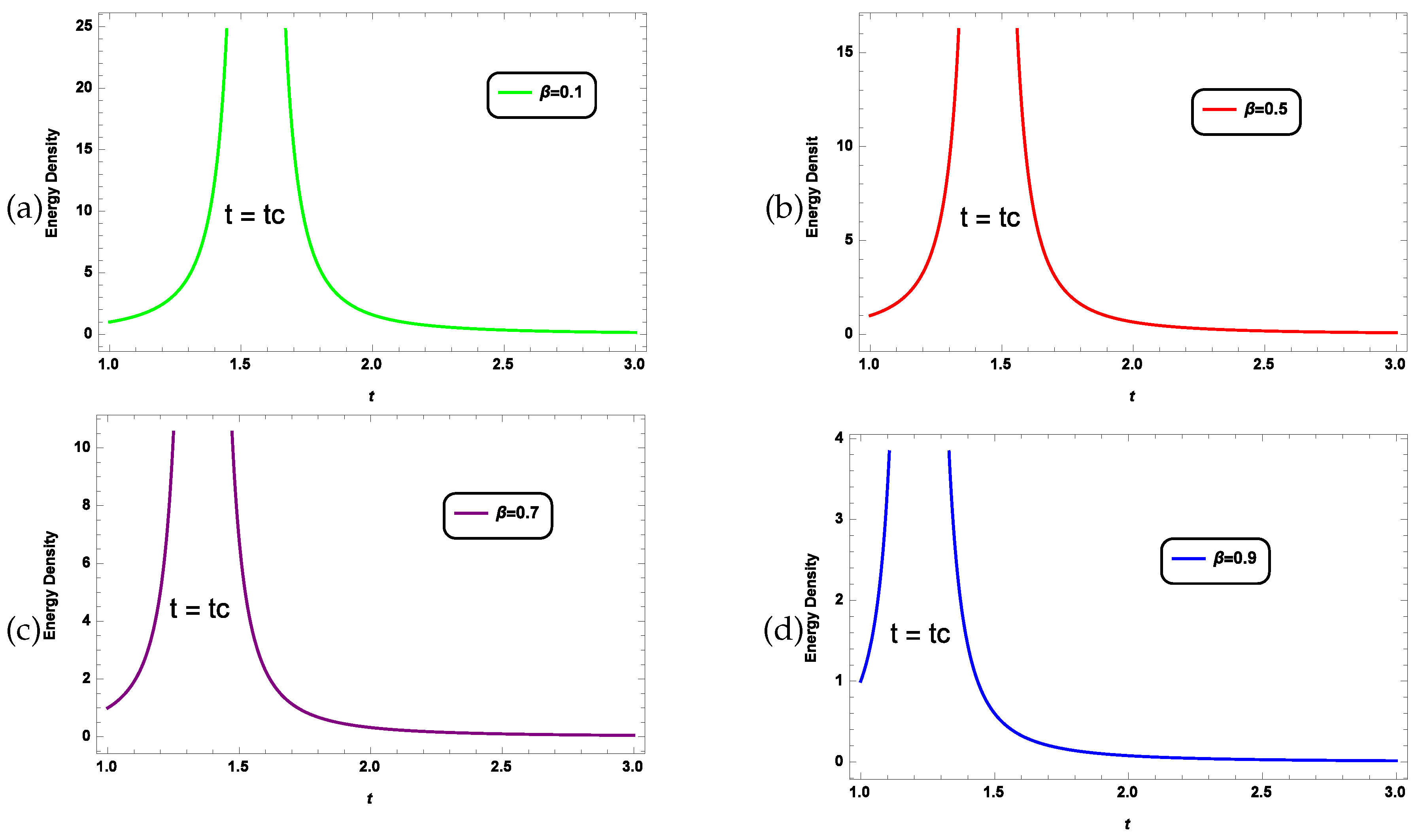
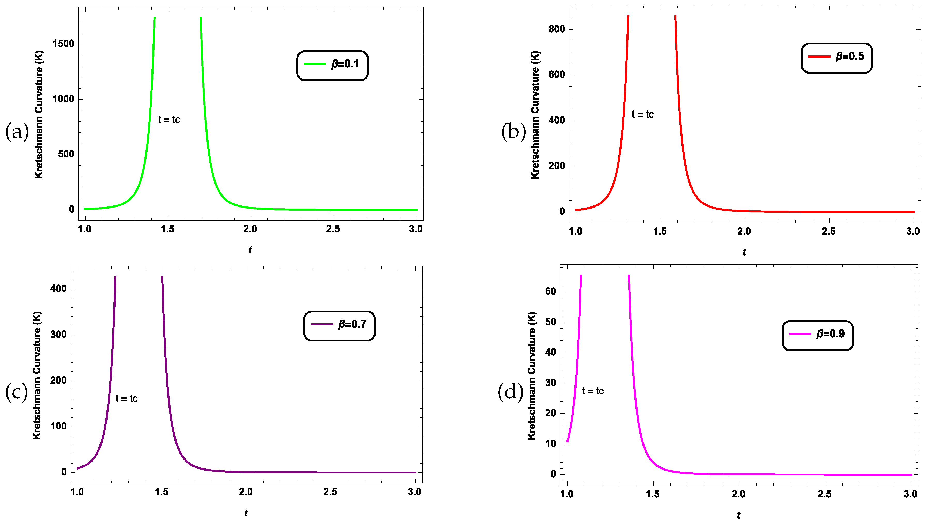
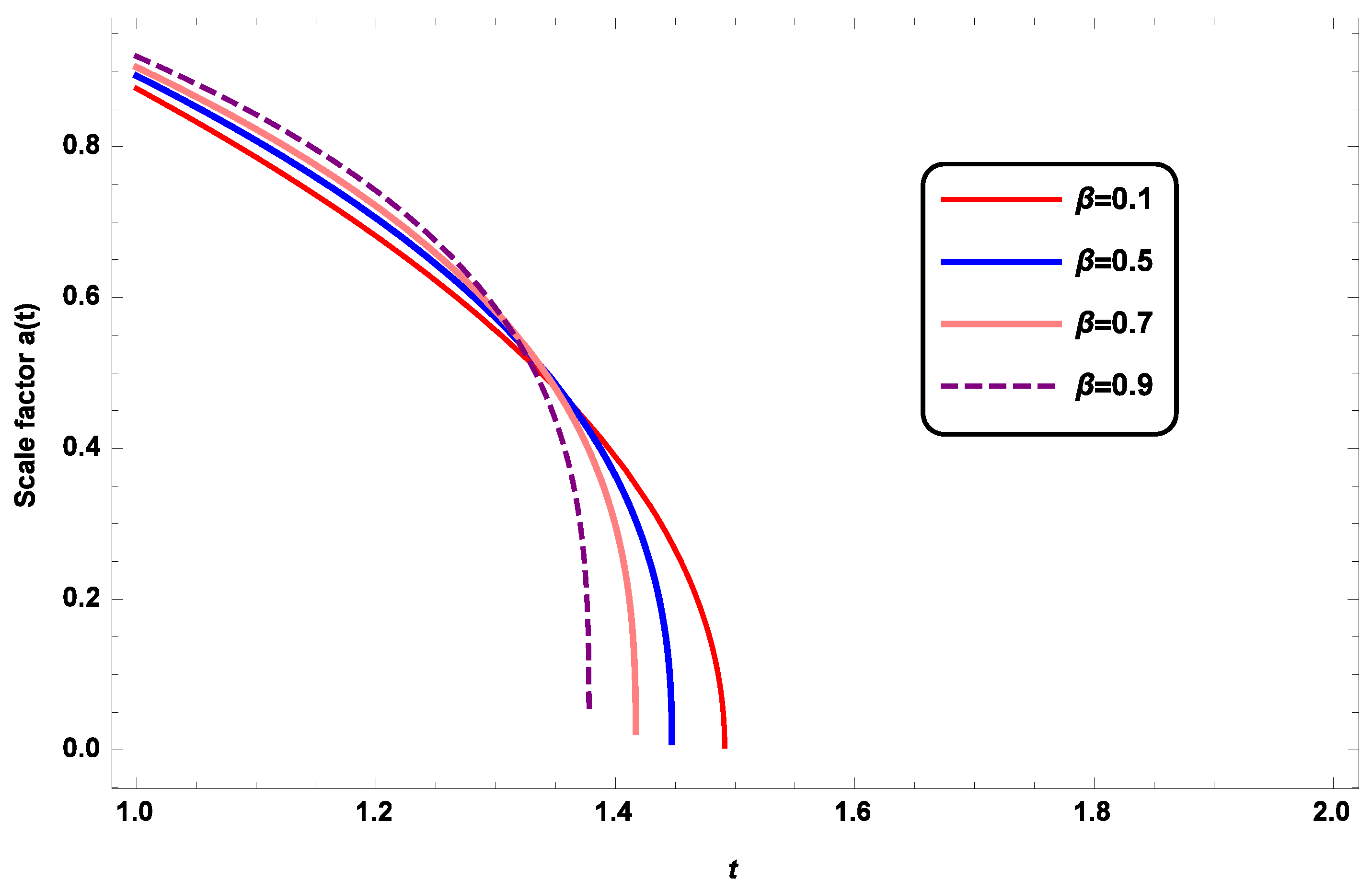
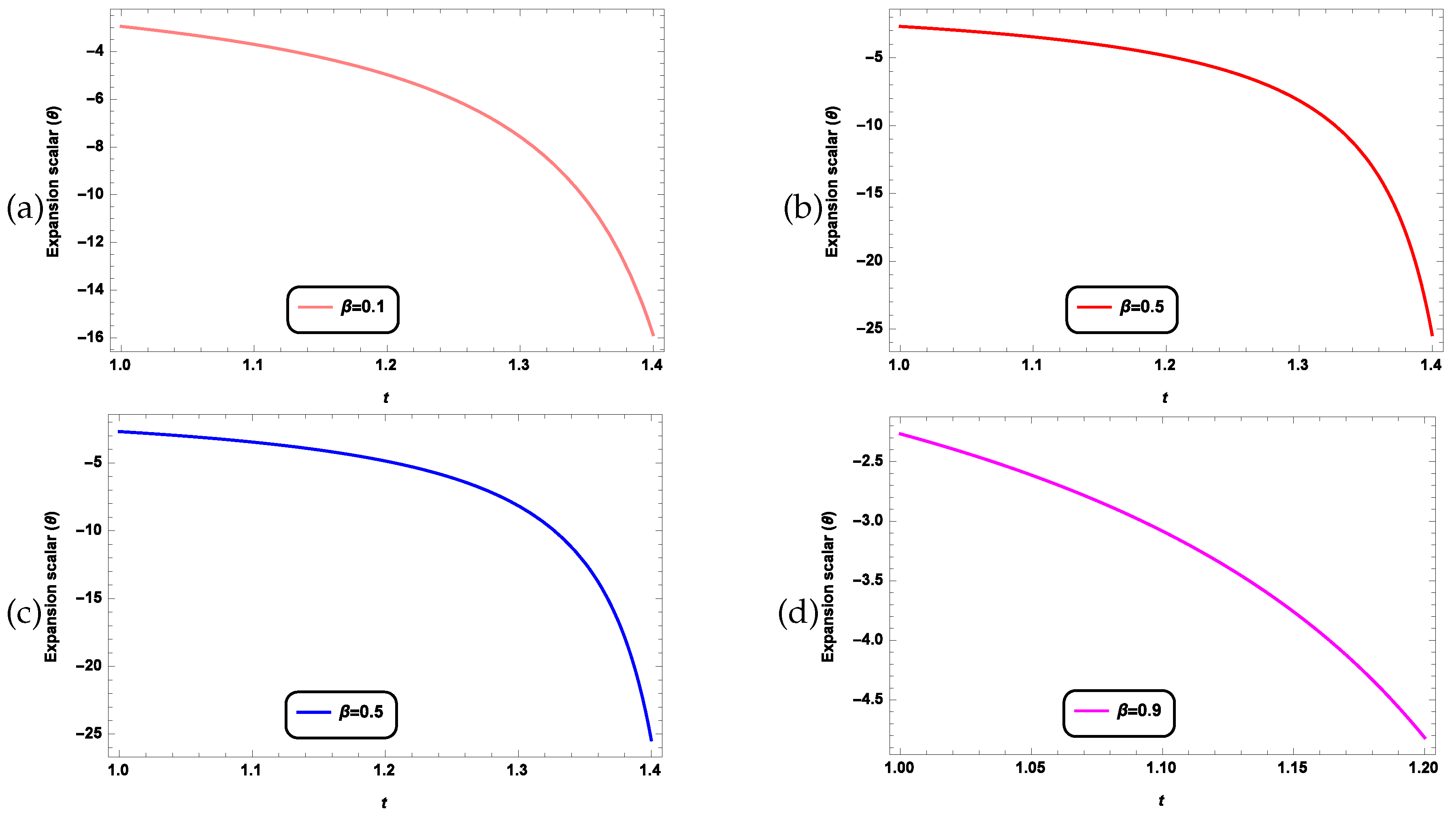
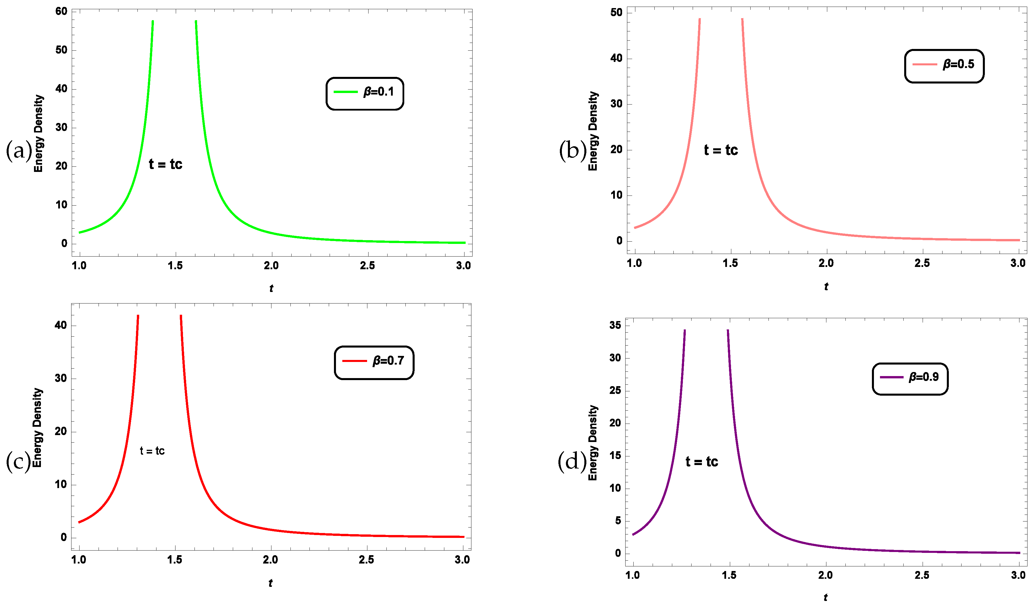
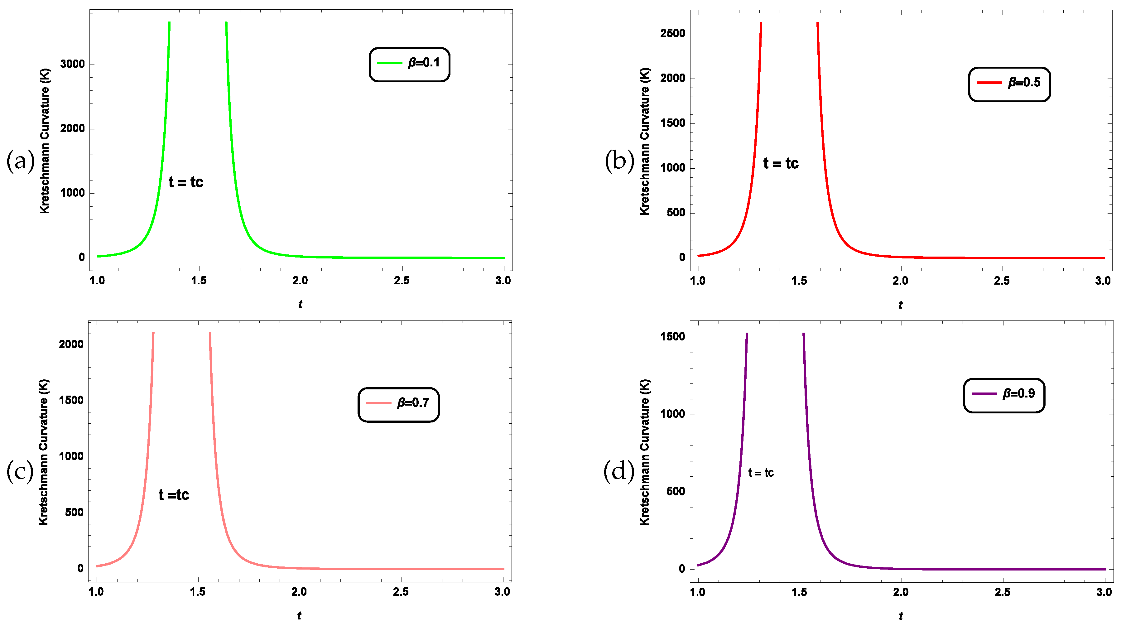
In Figure 1, we display the behaviour of scale factor a ( t ) with time coordinate t and observe that scale factor is monotonically decreasing in nature with time coordinate (t). In the same way, we display the behaviour of the expansion scalar ( Θ ), energy density ( ρ ) , and Kretschmann curvature ( K ) with time coordinate t for some estimated values of the model parameter β in Figure 2, Figure 3 and Figure 4 respectively.

4.2. ω = 1 3 (Radiation Fluid)

The Eos for ultra-relativistic `radiation’ is ω = 1 3 . In this case spacetime is dominated by radiation-induced pressure. In the case of radiative perfect fluid the energy density is propotional to 1 a 4 . In cosmology, for expnding universe the energy density of radiation decreases more quickly than the volume expansion, because its wavelength is red-shifted, whereas in collapsing scenerio expansion scalar decreses with time and energy density becomes divergent. Now in our model we consider the case of radiation fluid ( ω = 1 3 ) [23] and get the value of scale factor, energy density and other physical/geometrical parameters as:
a ( t ) = 2 3 ( 2 M ) 1 3 ( β 3 ) ( 2 β 1 ) k Λ 0 1 2 + 2 k ( t t 0 ) ( β 3 ) β 1 2 ( β 3 ) 2 ( 2 β 3 ) ( 3 β ) 3 k Λ 0 2 β + 3 12 ( β 3 ) 2 ( 2 β 1 ) 9 1 3 r 3 ( 2 β 1 ) 2 r 0 3 ( β 3 ) k 1 3
Θ = 3 k Λ 0 ( 2 β 1 ) 2 k Λ 0 ( t t 0 ) ( β 3 ) + { k ( 3 β ) Λ 0 ( 2 β 1 ) } 1 2
ρ = 3 k ( β 3 ) Λ 0 2 ( 2 β 1 ) { 2 k Λ 0 ( t t 0 ) ( β 3 ) + { k ( 3 β ) Λ 0 ( 2 β 1 ) } 1 2 } 2
p = k ( β 3 ) Λ 0 2 ( 2 β 1 ) { 2 k Λ 0 ( t t 0 ) ( β 3 ) + { k ( 3 β ) Λ 0 ( 2 β 1 ) } 1 2 } 2
and
K = 36 k 4 Λ 0 4 ( 2 β 1 ) 2 ( 9 6 β 2 β 2 ) { 2 k Λ 0 ( t t 0 ) ( β 3 ) + { k ( 3 β ) Λ 0 ( 2 β 1 ) } 1 2 } 4
In Figure 5, we display the behaviour of scale factor a ( t ) with time coordinate t and observe that scale factor is monotonically decreasing in nature with time coordinate (t). In the same way, we display the behaviour of the expansion scalar ( Θ ), energy density ( ρ ) , and Kretschmann curvature ( K ) with time coordinate t for some estimated values of model parameter β in Figure 6, Figure 7 and Figure 8 respectively.

4.3. Interpretation of the Graph and Estimation of the Model Parameter β

We observe from Figure 1, Figure 2, Figure 3 and Figure 4, Figure 5, Figure 6, Figure 7 and Figure 8 that in both cases for ω = 1 and ω = 1 3 , the nature of all physical and geometrical parameters ( ρ , K , a ( t ) , θ ) depends heavily on model parameter β . Singularity formation (black hole) is observed when 0 < β < 1 .
By assuming initial coordinates ( t 0 , r 0 ) = ( 1 , 1 ) , k = 1 , and r = 1 , and with the use of the above Equation (26), we have the areal radius (R) of the collapsing star as:
R ( t , r ) = r * a ( t ) = ( 2 M ) 1 3 β 3 3 β 7 1 3 , for ω = 1 . ( 2 M ) 1 3 9 9 β + 2 β 2 27 30 β + 8 β 2 1 3 , for ω = 1 3
by simplyfing Equation (35) we have
β = 7 R 3 M 6 3 R 3 M 2 , for ω = 1 . 6 10 R 3 M 6 ± 12 R 3 M 2 288 R 3 M + 144 16 2 R 3 M 1 , for ω = 1 3
As we observed from Equation (36), the model parameter β depends on the areal radius R and mass M of the collapsing star.
In the case of ω = 1 for R 3 M 6 7 , 1 ( 0 . 85 , 1 ) , the model parameter β takes the value in ( 0 , 1 ) for which we observed the singularity formation.
whereas in the case of ω = 1 3 for R 3 M 2 3 , 4 5 ( 0 . 66 , 0 . 8 ) the model parameter β takes the value in ( 0 , 1 ) for which we observed the singularity formation.
Although we will get the feasible solution of EFE’s for negative values of β , due to the dependency of β on the mass (M) and radius (R) of the star, it will be more realistic to consider only positive values.

5. Apparent Horizon and Singularity Analysis

A spacetime singularity is a disruption in spacetime caused by a breakdown in its geometry or in another fundamental physical component.When one or both of the geometrical and physical parameters, such as the energy density ( ρ ) and Kretschmann scalar curvature ( K ), begin to diverge, a spacetime singularity arises during the gravitational collapse process. The development of trapped surfaces in spacetime as a result of the gravitational collapse process will determine whether the singularity is a black hole (BH) or a naked singularity (NS). A naked singularity is a singularity without a boundary, while the formation of BH is identified by the development of an apparent horizon. Black holes are regions of spacetime from which nothing can escape, not even light rays. The gravitational attraction of a typical black hole is so strong that one would have to travel faster than light to escape its pull. When a star starts to collapse due to its own gravity, no portion of spacetime is trapped at first; however, as the collapse proceeds, density ( ρ ) becomes divergent and trapped surfaces begin to appear. In the BH scenerio, an apparent horizon is formed before the formation of a spacetime singularity. On the development of apparent horizons, we have
R , α R , β g α β = ( r a ˙ ) 2 1 = 0
If we assume that the collapsing star is not initially trapped at ( t 0 , r 0 ) , then we should have
R , α R , β g α β | ( t 0 , r 0 ) = ( r 0 a ˙ ( t 0 ) ) 2 1 < 0
by using the value of a ( t ) from Equation (21) in above Equation (37) we have the equation on the development of apparent horizon
( 2 M ) 2 3 ( β + β ω 2 ) 2 r A H 2 2 ( β 3 ) ω ( β + β ω 2 ) k Λ 0 1 2 + k ( t A H t 0 ) ( β 3 ) ( 1 + ω ) 2 + 6 ω ( 1 + ω ) ( β 3 ) = 2 ( β + β ω 2 ) ω ( 3 β ) k Λ 0 β + β ω + 6 ω 3 ( 1 + ω ) ( β 3 ) ( β + β ω 2 ) 2 3 r A H 3 ( β + β ω 2 ) 4 r 0 3 ω ( β 3 ) k 2 3
The time at which spacetime singularity forms is the time when energy density and kretschmann curvature diverges ( ρ , K ) at a finite time given by the use of Equation (24) as
t c = t 0 + 1 ( 1 + ω ) 2 ( β + β ω 2 ) ω k Λ 0 ( 3 β ) 1 2
The geometrical radius of apparent horizon surface is
R A H = r A H a ( t A H ) = r A H ( 2 M ) 1 3 2 ( β 3 ) ω ( β + β ω 2 ) k Λ 0 1 2 + k ( t A H t 0 ) ( β 3 ) ( 1 + ω ) β + β ω 2 ( 1 + ω ) ( β 3 ) 2 ( β + β ω 2 ) ω ( 3 β ) k Λ 0 β + β ω + 6 ω 6 ( 1 + ω ) ( β 3 ) ( β + β ω 2 ) 1 3 r A H 3 ( β + β ω 2 ) 4 r 0 3 ω ( β 3 ) k 1 3
from Equation (39) one can obtain the time ( t A H ) at which apparent horizon is developed given as
t A H = t 0 + ω ( 1 + ω ) 2 ω ( β + β ω 2 ) k Λ 0 ( 3 β ) 1 2 2 2 β ( 1 + ω ) + 3 ( 1 + 3 ω ) 3 ( 1 + 3 ω ) ( 3 β ) ω ( β + β ω 2 ) Λ 0 k 6 ω + β + β ω 1 + 3 ω 1 M 1 3 r A H ( β + β ω 2 ) ( 1 β + β 2 ) β ω ( 1 β β ω ) r 0 3 k ω ( β 3 ) ( β + β ω 2 ) 1 3 ( 1 + ω ) ( β 3 ) ( 1 + 3 ω )
with the use of Equation (40) and Equation (42) we obtain
t A H t c = t 0 + ω ( 1 + ω ) 2 ω ( β + β ω 2 ) k Λ 0 ( 3 β ) 1 2 2 2 β ( 1 + ω ) + 3 ( 1 + 3 ω ) 3 ( 1 + 3 ω ) ( 3 β ) ω ( β + β ω 2 ) Λ 0 k 6 ω + β + β ω 1 + 3 ω 1 M 1 3 r A H ( β + β ω 2 ) ( 1 β + β 2 ) β ω ( 1 β β ω ) r 0 3 k ω ( β 3 ) ( β + β ω 2 ) 1 3 ( 1 + ω ) ( β 3 ) ( 1 + 3 ω ) t 0 + 1 ( 1 + ω ) 2 ( β + β ω 2 ) ω k Λ 0 ( 3 β ) 1 2 1
For ω = 1 the development of apparent horizon is given as by assuming initial coordintes ( t 0 , r 0 ) = ( 1 , 1 ) , ω = 1 , k = 1 , Λ 0 = 1 and with the use of Equation (43) we obtain
t A H t c = ( 3 + β ) ( 1 + β ) 2 ( 3 + ( 3 + β ) ( 1 + β ) 3 4 β + β 2 ) [ 2 + 6 ( 3 + β ) ( 1 + β ) 2 ( 1 + β ) 2 ( 3 + β ) ( β 1 ) { ( 3 β ) ( 1 β ) } 3 3 + β + 2 9 β 6 M 3 β 6 ( β 1 ) 5 ( 3 β ) 12 ( β 3 ) β 15 12 { ( 3 β ) ( 1 β ) } 3 β 3 + 2 { ( 3 β ) ( 1 β ) } β β 3 + 2 β { ( 3 β ) ( 1 β ) } 3 β 3 + β 2 { ( 3 β ) ( 1 β ) } 3 β 3 ]
whereas For ω = 1 3 the development of apparent horizon is given as by assuming initial coordintes ( t 0 , r 0 ) = ( 1 , 1 ) , ω = 1 , k = 1 , Λ 0 = 1 and with the use of Equation (43) we obtain
t A H t c = ( 3 + β ) ( 6 + 4 β ) 2 { 18 18 β + 4 β 2 + ( 3 + 2 β ) ( 3 + β ) ( 3 + 2 β ) } [ 2 + 2 ( 3 2 β ) ( 3 β ) ( 3 2 β ) ( 3 + β ) ( 3 + 2 β ) + 1 ( 3 + β ) 2 2 ( 2 β ) 3 { ( 3 β ) ( 3 2 β ) } 3 + 2 β 18 ( 27 30 β + 8 β 2 ) 2 ( 3 + β ) 3 ]
The mass of the collapsing star on the apparent horizon region is
M A H = M r A H 3 2 ( 3 β ) ( β + β ω 2 ) Λ 0 k 1 2 + k ( t A H t 0 ) ( 1 + ω ) ( β 3 ) ( β + β ω 2 ) 2 ( β + β ω 2 ) ω ( 3 β ) k Λ 0 β + β ω + 6 ω 2 ( 1 + ω ) ( β 3 ) r A H 3 ( β + β ω 2 ) 4 r 0 3 ( β 3 ) ω k
Gravitational collapse phenomenon: Blackhole formation
We are assuming that the star starts to collapse at time t = t 0 , where Equation (38) holds, i.e., the collapsing star is not trapped at the initial moment t 0 . From Figure 3, Figure 4, Figure 7 and Figure 8, we can see that ρ , K at t = t c given in Equation (40). This time t c takes the finite values for ω = 1 , 1 3 and for all the β lies in ( 0 , 1 ) . It means the energy density and Kretschmann curvature diverge at a finite time t c , and hence a collapsing star forms a spacetime singularity at a finite time t c . Further, from Equations (44) and (45), we observe that the quantity t A H t c < 1 and takes finite values for all the β lies in ( 0 , 1 ) , i.e., apparent horizons form at finite time t A H and much earlier than collapse time t c . Thus, the spacetime singularity is not naked; it is covered by apparent horizons, i.e., the singularity will be a black hole.

6. Concluding Remarks

The aim of this work is to discuss singularity formation (BH) during the homogeneous gravitational collapsing phase of stellar systems and the final fate of the collapsing star. In this work, we have studied the gravitational collapse of a spherically symmetric star with a finite thickness filled with homogeneous and isotropic perfect fluid with EoS p = ω ρ in the context of classical general relativity. In general relativity, the exact solution of Einstien’s field equations (EFE) and studies of singularity formation are very essential, and very few models yield physically meaningful results in an astrophysical scenario. For our purposes, the exterior region of the star is assumed to be Schwartzchild-de Sitter/anti-de Sitter, while the interior of the star is assumed to be the FLRW metric. We have used Λ parameterization to obtain the exact solution of field equations because the dynamical character of the cosmological constant is preferred in the recent cosmological model rather than the constant behaviour of the cosmological onstant. The dynamical Λ ( t ) model is assumed to be in the form Λ = β Θ ˙ 3 + Θ 2 9 . By using this parametrization, we were able to solve the field equation and, as a result, ascertain the dynamical evolution of the collapse process. We use this parametrization and junction conditions to obtain the exact solution of EFE’s in terms of the mass of the star (M) and radius (R). We have obtained a relation between the mass (M) and radius (R) of a star for which this model forms a spacetime singularity (BH). The two cases of gravitational collapse have been discussed: the first is for ω = 1 , which is the case of stiff matter, and the second is for ω = 1 3 , i.e., the case of radiation fluid. We have calculated all the physical and geometrical quantities ( ρ , p , θ , K ) for our model in terms of M and R. We observed that the nature and final fate of collapsing stars heavily depend on the model parameter β , which has been evaluated in terms of M and R, i.e., the collapse ultimately depends on the masses and radii of collapsing stars. In the case of ω = 1 for R 3 M 6 7 , 1 ( 0 . 85 , 1 ) ,and ω = 1 3 for R 3 M 2 3 , 4 5 ( 0 . 66 , 0 . 8 ) , and for these ranges, model parameter β takes the value in ( 0 , 1 ) for which we observed the singularity formation. We will get the feasible solution of EFE’s for negative values of β ; due to the dependency of β on the mass (M) and radius (R) of the star, it will be more realistic to consider only positive values. Using the graphical representation of the model, we have examined the collapsing configuration as follows:
  • The scale factor a ( t ) takes the finite value for given masses of considered stars and is monotonically decreasing in nature Figure 1 and Figure 5.
  • The expansion scalar Θ is negatively increasing with time coordinate t, which shows that collapsing phenomena occur and the motion of collapsing fluid towards the core of the star (Figure 2) and (Figure 6).
  • The graphical representation of energy density ( ρ ) Figure 3 and Figure 7, and Kretschmann curvature ( K ) Figure 4 and Figure 8 shows that both take positive and finite values for given masses of stars. Both are increasing in nature, and at a finite time t c , both become divergent, which shows singularity formation.
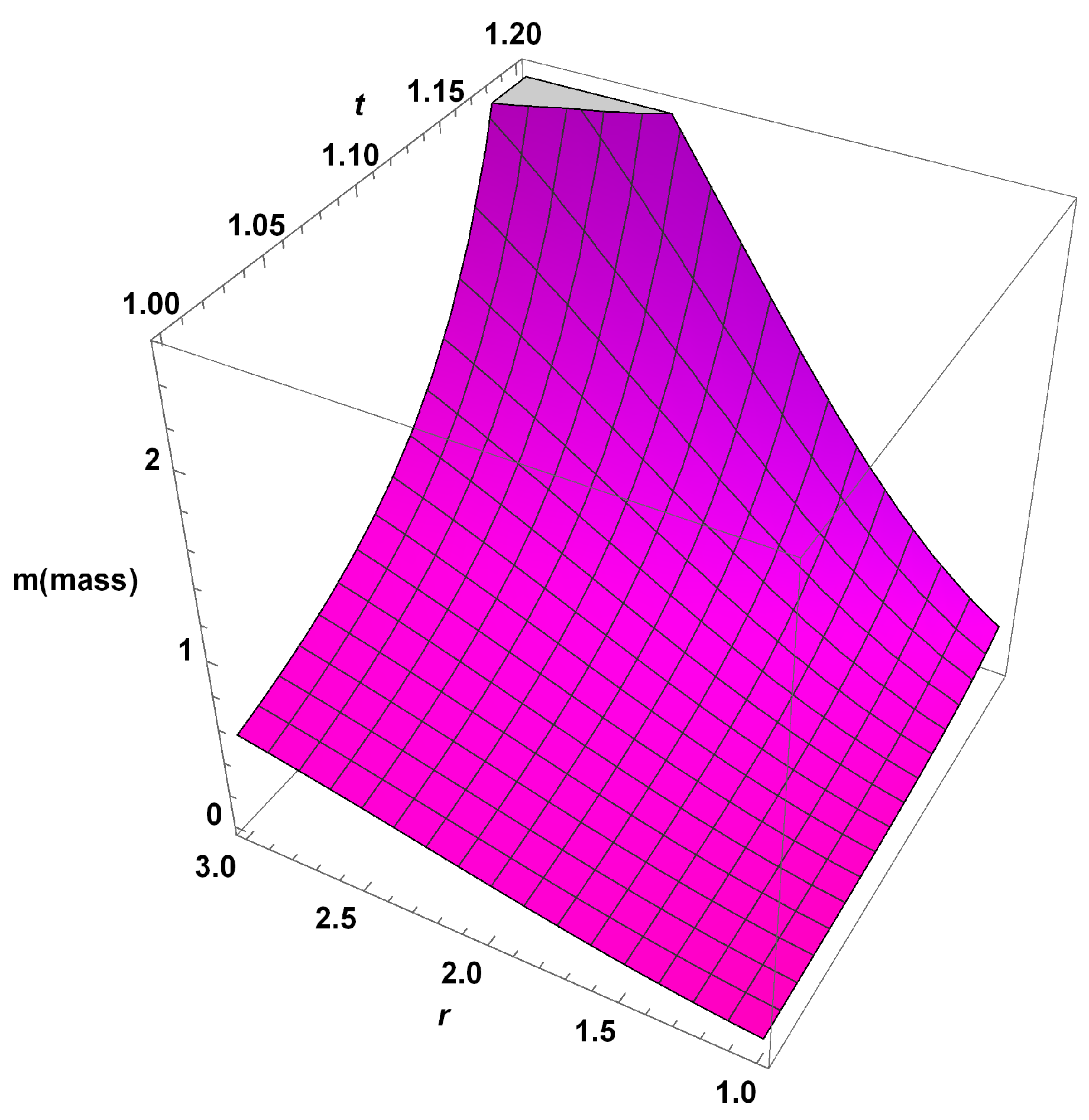
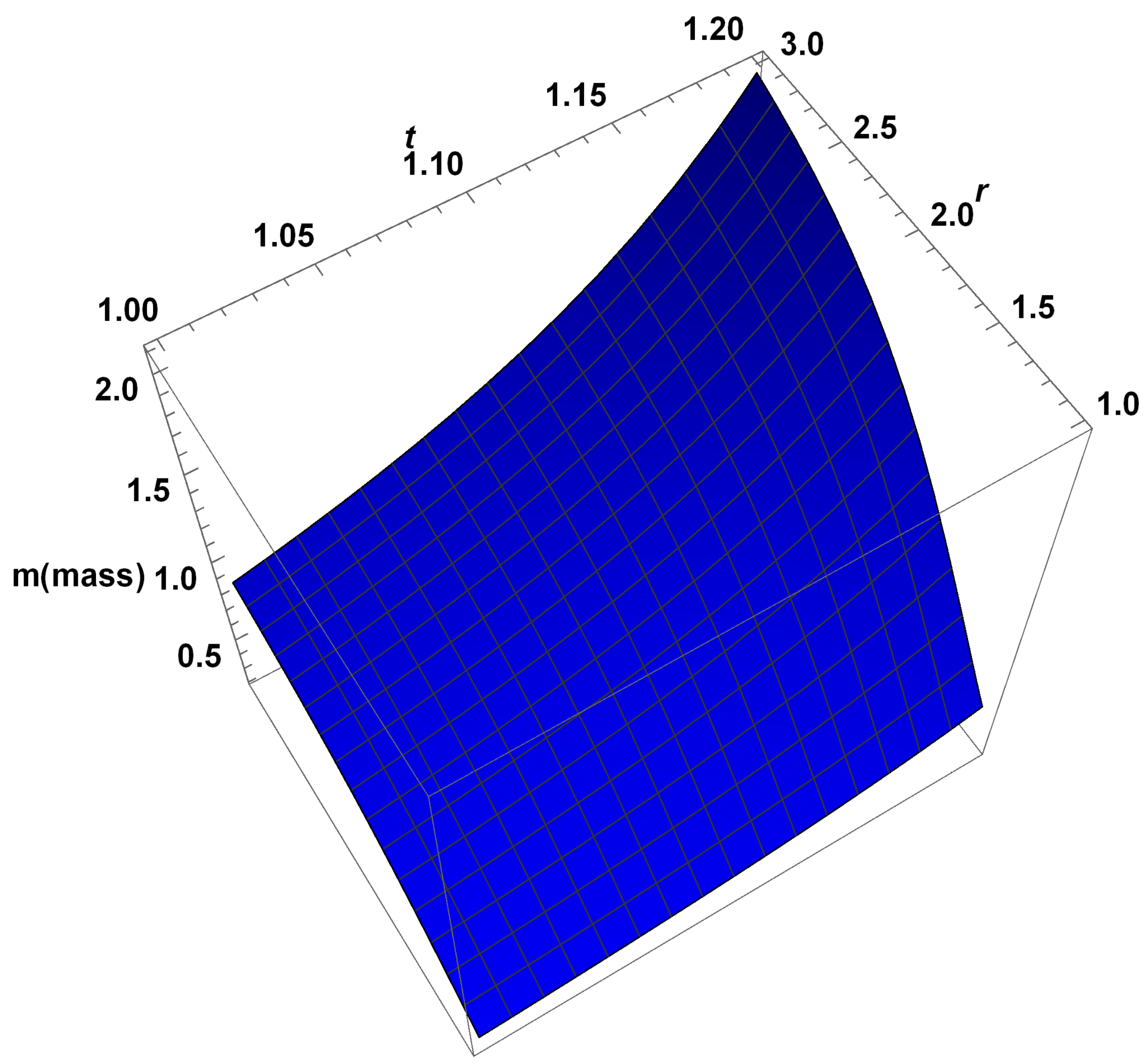
  • The graph of the mass function shows that it is regular, finite, and decreasing with time t and radial coordinate r Figure 9 and Figure 10. In classical mechanics, an absolute ground state is defined by E = 0 , which means if a star truly becomes BH, then E = M c 2 = 0 , i.e., M 0 . The mathematical "black hole" solution accurately predicts that a black hole (BH) may have an infinitesimally small mass [38]. In general theory of relativity, a M 0 event doesn’t demonstrate the absence of matter, as gravitational mass comprises all sources of energy, including negative self-gravitational energy. Therefore, this phenomenon could be a sign of extreme self-gravitation, counteracting internal energies like heat and pressure as well as external energy sources like protons and neutrons.
The development of an apparent horizon for a collapsing star has been studied in Equation (39). Also, the mass ( M A H ) of a collapsing star in the apparent horizon region has been calculated in Equation (46). To predict whether a black hole is formed or not, we have calculated the quantity t A H t c and observed that for the estimated value of model parameter β , the value t A H t c < 1 suggested that the apparent horizon developed before the collapse time t c , and as blackholes must be hidden behind the apparent horizon, both cases (stiff matter and radiation fluid) lead to the formation of Blackholes.

Author Contributions

Conceptualization, A.P.; methodology, A.P.; software, A.P.; validation, A.P., and S.K.S.; formal analysis, A.P.; investigation, A.P.; resources, A.P. and S.K.S; data curation, A.P.; writing—original draft preparation, A.P.; writing—review and editing, A.P.; visualization, A.P. and S.K.S.; supervision, S.K.S; funding acquisition, A.P. All authors have read and agreed to the published version of the manuscript.

Funding

This research was funded by Department of Science and Technology (DST) OF FUNDER grant number IF190267.

Data Availability Statement

The data is available upon request from the authors.

Acknowledgments

The first author A.P. is thankful to DST-Inspire Fellowship, Govt. of India for financial assistance.

Conflicts of Interest

The authors declare no conflict of interest.

References

  1. Oppenheimer, J.R.; Snyder, H. On Continued Gravitational Contraction. Phys. Rev. B 1939, 56, 455–459, . [CrossRef]
  2. SR Maiti. Fluid with heat flux in a conformally flat space-time. Physical Review D, 25(10):2518, 1982.
  3. Modak, B. Cosmological solution with an energy flux. J. Astrophys. Astron. 1984, 5, 317–322, . [CrossRef]
  4. Banerjee, A.; Choudhury, S.B.D.; Bhui, B.K. Conformally flat solution with heat flux. Phys. Rev. D 1989, 40, 670–672, . [CrossRef]
  5. Schäfer, D.; Goenner, H.F. The Gravitational Field of a Radiating and Contracting Spherically-Symmetric Body with Heat Flow. Gen. Relativ. Gravit. 2000, 32, 2119–2130, . [CrossRef]
  6. BVIvanov. Collapsing shear-free perfect fluid spheres with heat flow. General Relativity and Gravitation, 44(7):1835–1855, 2012.
  7. Herrera, L.; LE Denmat, G.; Santos, N.O.; Wang, A. SHEAR-FREE RADIATING COLLAPSE AND CONFORMAL FLATNESS. Int. J. Mod. Phys. D 2004, 13, 583–592, . [CrossRef]
  8. Chakrabarti, S.; Banerjee, N. Scalar field collapse in a conformally flat spacetime. Eur. Phys. J. C 2017, 77, 166, . [CrossRef]
  9. R.G.Cai, Li-Wei Ji and Run-Qiu Yang. Collapse of Self-interacting scalar field in Anti-de Sitter space, Communication in Theoretical Physics,63(3), 329(2016).
  10. R.Zacharias, Relativistic gravitational collapse by thermal mass, Communication in Theoretical Physics, 73(1), 015401 (2020).
  11. Liddle, A.R.; Scherrer, R.J. Classification of scalar field potentials with cosmological scaling solutions. Phys. Rev. D 1998, 59, 023509, . [CrossRef]
  12. Steinhardt, P.J.; Wang, L.; Zlatev, I. Cosmological tracking solutions. Phys. Rev. D 1999, 59, 123504, . [CrossRef]
  13. Dvali, G.; Gabadadze, G.; Porrati, M. 4D gravity on a brane in 5D Minkowski space. Phys. Lett. B 2000, 485, 208–214, . [CrossRef]
  14. Deffayet, C. Cosmology on a brane in Minkowski bulk. Phys. Lett. B 2001, 502, 199–208, . [CrossRef]
  15. Malafarina, D.; Toshmatov, B.; Dadhich, N. Dust collapse in 4D Einstein-Gauss-Bonnet gravity. Phys. Dark Universe 2020, 30, 100598, . [CrossRef]
  16. N.Banrejee, and T.Paul, scalar field collapse in GaussBonnet gravity, Eur. Phys. J. C 78 (2)(2018) 1-6.
  17. Cline, J.M.; Vinet, J. Problems with time-varying extra dimensions or “Cardassian expansion” as alternatives to dark energy. Phys. Rev. D 2003, 68, 025015, . [CrossRef]
  18. Yungui Gong, Anzhong Wang, and Qiang Wu. Cosmological constant and late transient acceleration of the universe in the horavawitten heterotic m theory on s1/z2. Physics Letters B, 663(3):147?151, 2008.
  19. Pereira, P.R.; DA Silva, M.F.A.; Chan, R. ANISOTROPIC SELF-SIMILAR COSMOLOGICAL MODEL WITH DARK ENERGY. Int. J. Mod. Phys. D 2006, 15, 991–999, . [CrossRef]
  20. Riess, A.G., et al. [Supernova Search Team Collaboration], Astron. J. 116, 1009 (1998) [arXiv:astro-ph/9805201]; S. Perlmutter et al. [Su- pernova Cosmology Project Collaboration], Astrophys. J. 517, 565 (1999) [arXiv:astro-ph/9812133]; A. G. Riess et al. [Supernova Search Team Collaboration], Astro- phys. J. 607, 665 (2004) [arXiv:astro-ph/0402512].
  21. Ray, S.; Bagla, J.S.; Padmanabhan, T. Gravitational collapse in an expanding universe: scaling relations for two-dimensional collapse revisited. Mon. Not. R. Astron. Soc. 2005, 360, 546–554, . [CrossRef]
  22. Brandt, C.F.C.; Chan, R.; da Silva, M.A.F.; da Rocha, J.F.V. Inhomogeneous dark energy and cosmological acceleration. Gen. Relativ. Gravit. 2007, 39, 1675–1687, . [CrossRef]
  23. Campos, M.; Lima, J.A.S. Black hole formation with an interacting vacuum energy density. Phys. Rev. D 2012, 86, . [CrossRef]
  24. M Campos, Gravitational collapse and the vacuum energy 2014 J. Phys.: Conf. Ser. 496 012021, doi:10.1088/ 1742-6596/496/1/012021.
  25. Wang, P.; Meng, X.-H. Can vacuum decay in our universe?. Class. Quantum Gravity 2004, 22, 283–294, . [CrossRef]
  26. Shah, H.H.; Rahaman, F.; Ali, A.; Molla, S. Gravitational collapse of an interacting vacuum energy density with an anisotropic fluid. Phys. Dark Universe 2019, 24, 100291, . [CrossRef]
  27. S. Ray et al., Int. J. Theor. Phys. 48(9), 2499 (2009).
  28. Cahill, M. E.,& McVittie, G. C. (1970). Spherical Symmetry and Mass- Energy in General Relativity. I. General Theory. Journal of Mathematical Physics, 11(4), 1382-1391.
  29. T.A.Madhav, R. Goswami and P.S. Joshi, Gravitational; collapse in asymptotixally anti de Sitter or de Sitter backgrounds, phys. Rev. D72(8)(2005)084029.
  30. D. Malafarina and P.S. Joshi, Gravitational collapse with tengential pressure, Int. J. Mod Phys. D20(4)(2011) 463-495.
  31. Israel, W. Singular hypersurfaces and thin shells in general relativity. Il Nuovo Cimento B 1966, 44, 1–14, . [CrossRef]
  32. Bonnor, W.B.; Vickers, P.A. Junction conditions in general relativity. Gen. Relativ. Gravit. 1981, 13, 29–36, . [CrossRef]
  33. Cherubini, C.; Bini, D.; Capozziello, S.; Ruffini, R. SECOND ORDER SCALAR INVARIANTS OF THE RIEMANN TENSOR: APPLICATIONS TO BLACK HOLE SPACETIMES. Int. J. Mod. Phys. D 2002, 11, 827–841, . [CrossRef]
  34. Misner, C.W.; Sharp, D.H. Relativistic Equations for Adiabatic, Spherically Symmetric Gravitational Collapse. Phys. Rev. B 1964, 136, B571–B576, . [CrossRef]
  35. Doroshkevich, A. G., Zel’dovich, Y. B.,& Novikov, I. D. (1968). Weakly interacting particles in the anisotropic cosmological model. Soviet Physics JETP, 26(2).
  36. Oliveira-Neto, G.; Monerat, G.A.; Silva, E.V.C.; Neves, C.; Filho, L.G.F. AN EARLY UNIVERSE MODEL WITH STIFF MATTER AND A COSMOLOGICAL CONSTANT. Int. J. Mod. Physics: Conf. Ser. 2011, 03, 254–265, . [CrossRef]
  37. Pandey, A.; Kumar, R.; Srivastava, S.K. Shear-free gravitational collapse of dust cloud and dark energy. Int. J. Geom. Methods Mod. Phys. 2022, 19, . [CrossRef]
  38. Mitra, A. On the non-occurrence of Type I X-ray bursts from the black hole candidates. Adv. Space Res. 2006, 38, 2917–2919, . [CrossRef]
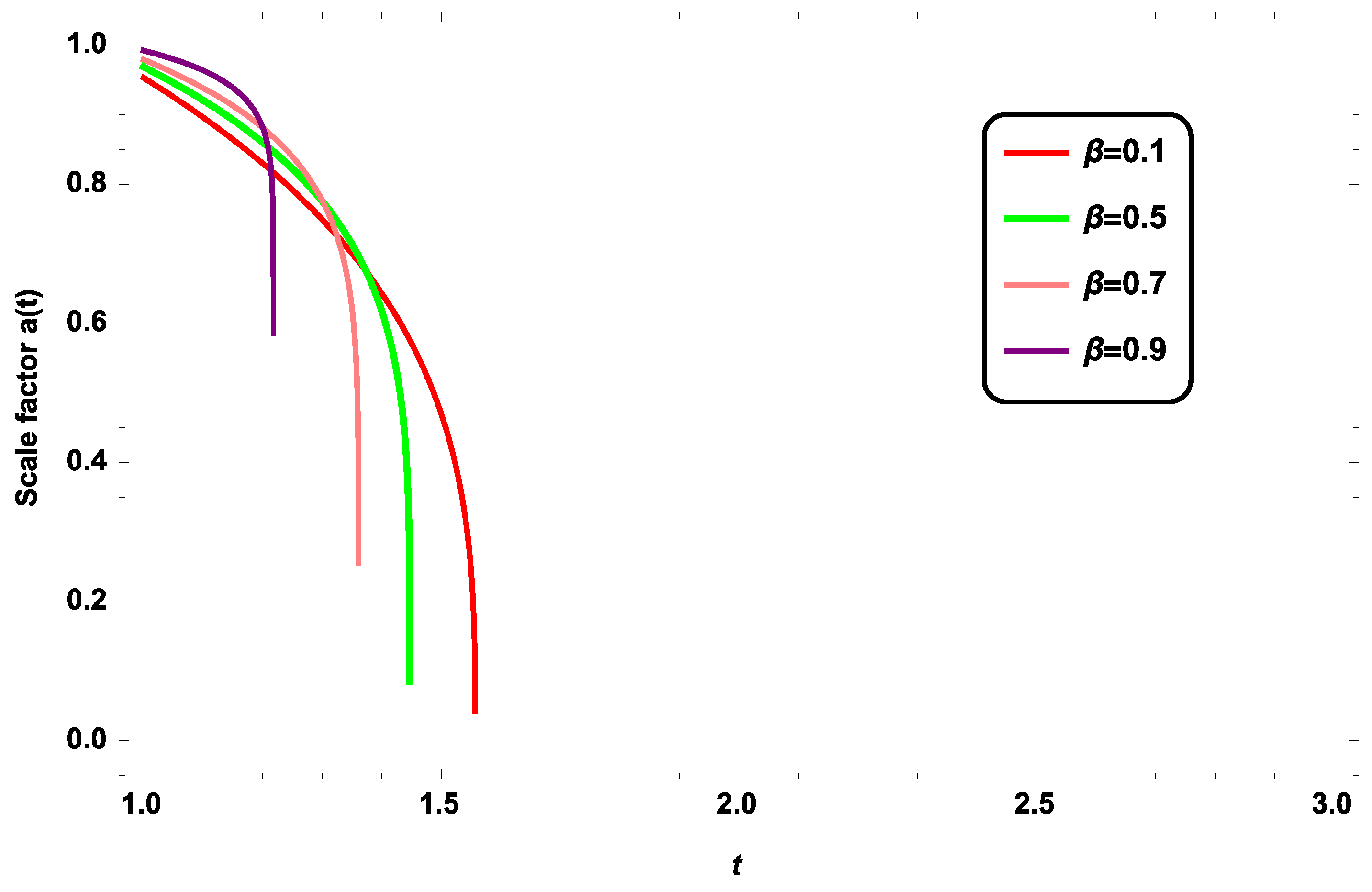
Figure 1. Collapsing configuration: The scale factor a ( t ) given in Equation (26) is plotted with respect to time coordinate t for four values of model parameter β and for ω = 1 with initial coordinate ( t 0 , r 0 ) = ( 1 , 1 ) .
Preprints 111196 g001
Figure 2. Collapsing configuration: The expansion scalar ( Θ ) given in Equation (27) is plotted with respect to time coordinate t for four values of model parameter β and ω = 1 with initial coordinate ( t 0 , r 0 ) = ( 1 , 1 ) .
Preprints 111196 g002
Figure 3. The energy density ( ρ ) given in Equation (28) is plotted with time coordinate t for four values of model parameter β and ω = 1 with initial coordinate ( t 0 , r 0 ) = ( 1 , 1 ) .
Preprints 111196 g003
Figure 4. The Kretschmann curvature ( K ) given in Equation (29) is plotted with time coordinate t for four values of model parameter β and ω = 1 , with initial coordinate ( t 0 , r 0 ) = ( 1 , 1 ) .
Preprints 111196 g004
Figure 5. Collapsing configuration: The scale factor a ( t ) given in Equation (30) is plotted with respect to time coordinate t for four values of model parameter β and for ω = 1 3 with initial coordinate ( t 0 , r 0 ) = ( 1 , 1 ) .
Preprints 111196 g005
Figure 6. Collapsing configuration: The expansion scalar ( Θ ) given in Equation (31) is plotted with respect to time coordinate t for four values of model parameter β and for ω = 1 3 with initial coordinate ( t 0 , r 0 ) = ( 1 , 1 ) .
Preprints 111196 g006
Figure 7. The energy density ( ρ ) given in Equation (32) is plotted with time coordinate t for four values of model parameter β and for ω = 1 3 , with initial coordinate ( t 0 , r 0 ) = ( 1 , 1 ) .
Preprints 111196 g007
Figure 8. The Kretschmann curvature ( K ) given in Equation (34) is plotted with time coordinate t for four values of model parameter β and for ω = 1 3 with initial coordinate ( t 0 , r 0 ) = ( 1 , 1 ) .
Preprints 111196 g008
Figure 9. The mass function ( M A H ) given is plotted with time coordinate t radial coordinate r and for β = 0 . 9 (corresponding to ω = 1 ) with initial coordinate ( t 0 , r 0 ) = (1,1).
Preprints 111196 g009
Figure 10. The mass function ( M A H ) given is plotted with time coordinate t radial coordinate r and for β = 0 . 9 (corresponding to ω = 1 3 ) with initial coordinate ( t 0 , r 0 ) = (1,1).
Preprints 111196 g010
Disclaimer/Publisher’s Note: The statements, opinions and data contained in all publications are solely those of the individual author(s) and contributor(s) and not of MDPI and/or the editor(s). MDPI and/or the editor(s) disclaim responsibility for any injury to people or property resulting from any ideas, methods, instructions or products referred to in the content.
Copyright: This open access article is published under a Creative Commons CC BY 4.0 license, which permit the free download, distribution, and reuse, provided that the author and preprint are cited in any reuse.
Prerpints.org logo

Preprints.org is a free preprint server supported by MDPI in Basel, Switzerland.

Subscribe

© 2024 MDPI (Basel, Switzerland) unless otherwise stated