1. Introduction
Crop water requirements form the major basis for irrigation water management. Evapotranspiration (ET), a word used to describe the combined processes of evaporation and transpiration from the surface of the soil and plant leaves, respectively, is measured by crop water requirement. The evaporation from the soil surface and the transpiration from plant stomatal activity are combined in the ET, a bio-physical process [
1]. One of the most crucial elements of the hydrologic cycle and the water balance model is the process of determining ET. Numerous researches, including hydrologic water balance, crop yield simulation, irrigation system design and management, and planning and management of water resources, depend on its precise estimation.
An empirical crop coefficient (Kc) is used to moderate the estimated reference evapotranspiration (ETo) from a standard surface, which is a typical method for predicting ET at any given time for a particular crop. Even though a lysimeter is the optimal tool for measuring ETo, this strategy is not always feasible because to its time-consuming, expensive, and need for extensive fieldwork as well as careful observation. Because ETo data is widely used in agriculture and hydrology studies, over the past 70 years, a number of studies and research projects have focused on developing various types of mathematical models to indirectly estimate the ETo and enhance the performance of these models. The literature [
2] offers a variety of indirect ETo estimation methods, from empirical to complicated models. However, the choice of appropriate models for ET estimation is contingent upon the data at hand, the features of the region, and the level of accuracy required. A sophisticated method known as the Penman-Monteith model [
3,
4,
5,
6] makes use of the physical properties of the ET process, such as heat and mass balance, by fusing energy and aerodynamic terms. This approach is acknowledged as the most effective worldwide method for estimating ETo in situations where measured ETo values are unavailable [
7,
8]. Moreover, a number of numerical models are calibrated and validated using P-M calculated ETo as the base method.
Because machine learning and artificial intelligence-based numerical approaches can map the input-output relationship without requiring a deep understanding of the underlying physical process, they have become increasingly used in evapotranspiration estimation over the past 20 years [
9,
10,
11,
12]. This has led to a reduction in complexity. The use of these machine learning techniques to modelling and evapotranspiration estimate has produced a number of success stories. With the introduction of the neural network model and its numerous variations, the use of advanced computational capabilities in the estimation of evapotranspiration was initiated [
13,
14,
15,
16,
17,
18,
19,
20,
21,
22,
23,
24,
25,
26,
27,
28].
The ANN model further improved to the algorithm of support vector machine (SVM) which was (i) less complex structure, (ii) less data requirement for training, (iii) very fast in data training/learning (iv) parameter optimization with less risk of learning function’s local minimum unlike ANN and (v) less sensitive to initial randomization of the weight matrix. Thus, in the last decade, much of the focus shifted to the implementation of the SVM algorithm in modelling the evapotranspiration process [
29]. But since 2015, simulating the evapotranspiration process with deep learning and extreme learning techniques has received a lot of interest. The decision tree method of the classification and regression tree (CART) type was primarily used in this technique [
30,
31,
32,
33,
34]. However, by using the more reliable ensembled machine learning approach, the performance could be improved even more. The boosting techniques utilized in this ensembled machine learning approach further enhance the learning performance algorithm [
35].
The focus of this study is on how different machine learning algorithms, including Random Forest, Gradient Boosting Machine (GBM), and Extreme Gradient Boosting Machine (XGBoost), perform in relation to one another. The application of these techniques and their comparative impact on the mapping ability of the evapotranspiration process is not been explicitly demonstrated in the literature [
31,
36,
37,
38,
39,
40,
41,
42,
43]. Additionally, there are limited or no study has been carried out in the past to explore the generalization capabilities of these models based on machine learning approaches. This is particularly important because once these models can be generalized, they can be directly implemented in the location, where past data are unavailable to develop locally trained models. The current study summarizes the comparative effectiveness of these techniques in estimating the ETo for locations whose data are not included in the model training and validation, in addition to reporting the successful implementation of these enhancements in the modelling of the evapotranspiration process.
2. Materials and Methods
2.1. Location
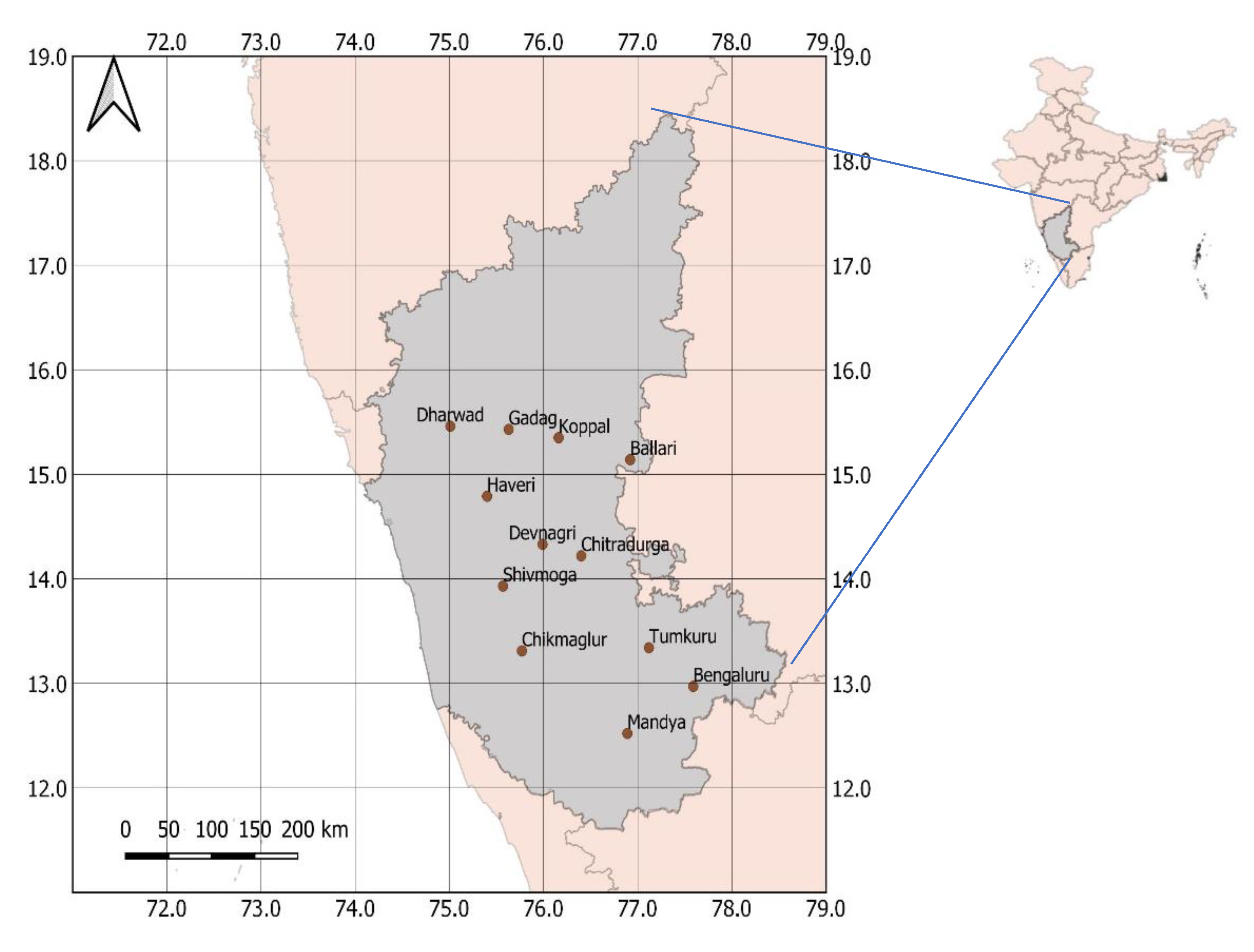
The different locations selected for the present study represent the Karnataka state of India which mostly falls under Agro-Ecological Zone 10 called as Southern Plateau and Hill region in the Indian sub-continent (
Figure 1). This region is spread to the extent of 11.30
oN to 18.30
oN and 74.0
oE to 74.30
oE and the area of the region is 19.20 million ha. The climate is typically semi-arid with 69% of the cultivable area comes under dryland agriculture. The major soil types include sandy loam, red calcareous and black soils. The region receives meagre annual rainfall ranging between 500-700 mm compelling inhabitant farmers (mostly small and marginal farmers owning less than 1 ha of culturable land) practicing sustenance farming due to low cropping intensity and agricultural productivity. Thus, water management at a regional scale assumes a key factor in sustainable and enhanced farm production in this region. The important crops grown in this region include Cotton, Jowar, Bajra, Groundnut, Millets, Banana, Turmeric, Onions, and Chilies along with fodder crops.
2.2. Data Set and Methodology
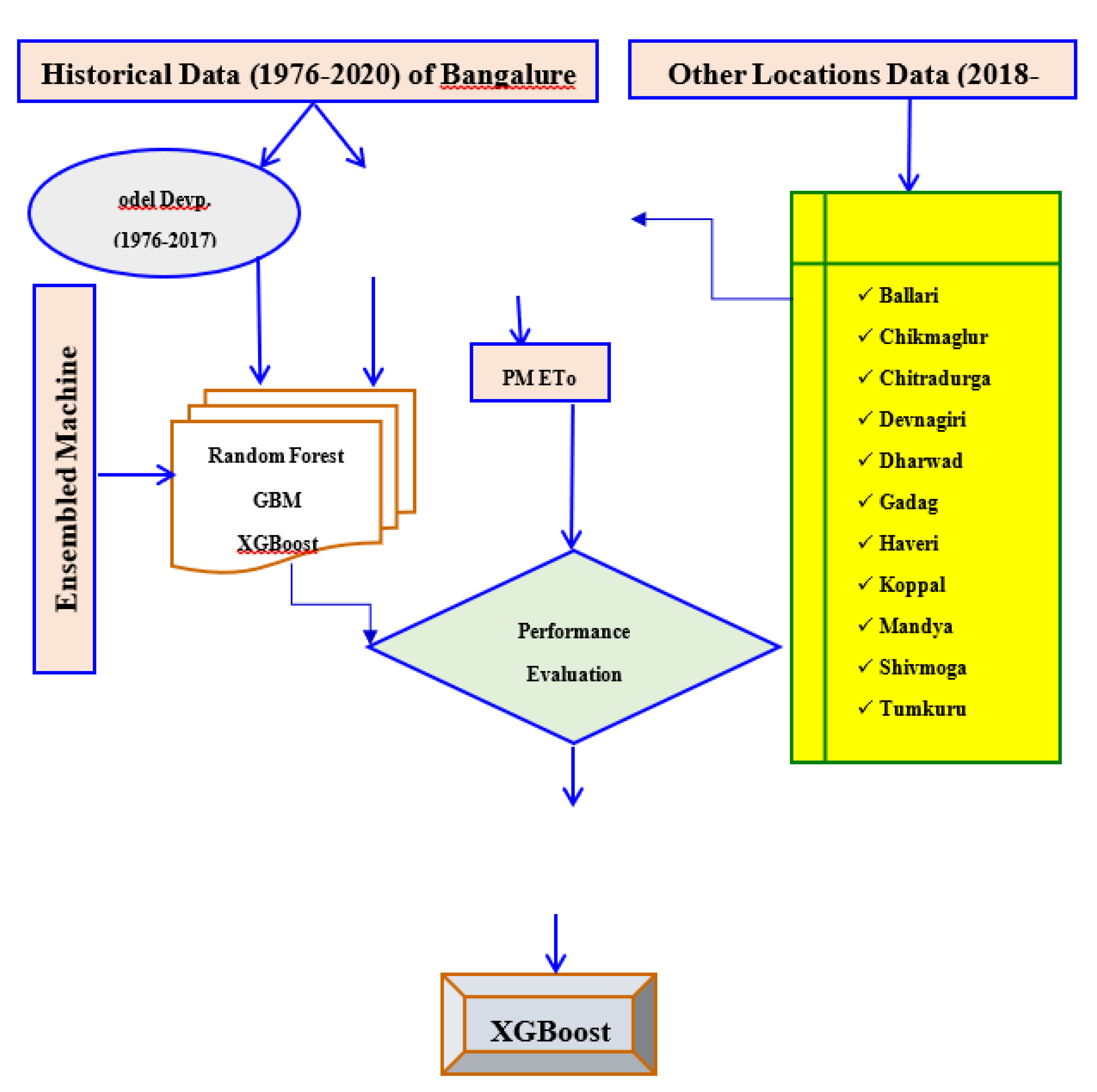
Figure 2 depicts the detailed methodology. For the meteorological station Bengaluru in the Indian state of Karnataka, daily meteorological data for fundamental climatic parameters such minimum and maximum temperature, minimum and maximum relative humidity, wind speed, solar radiation, and rainfall were gathered (
Figure 1). Numerical values for Julian Days (1-365), months (1 to 12 respectively for January to December), and quarters (1 to 4 respectively for January-March; April-June; July-September and October-December) were also included in the input data set in order to capture the monthly and seasonal variation in the underlying evapotranspiration process. The chosen stations represent the Agro-climatic zone of the Southern Plateau and Hill in the Indian subcontinent. The 44 years of daily data correspond to all the basic parameters for the duration of January 01, 1976 to June 30, 2020 were used in the development and validation of models. As recommended by [
5], a data quality check was carried out, and incorrect and missing records were excluded from the model training, validation, and testing phases. The data was divided into input data for validation (testing the model) and input data for learning (used for developing the model).
Table 1 contains information about the different locations.
The models were developed using the climatic data of Bengaluru stations with corresponding PM ETo values as targets. For this purpose, daily records for the duration January 01, 1976 to December 31, 2017 excluding the incomplete and erroneous daily records were considered. For model testing, daily records from January 01, 2018 to June 30, 2020 were considered. The model thus developed was directly applied to 11 other locations that were not included in model development. In these locations, developed models were tested using the daily records from January 01, 2018 to June 30, 2020 as is the case with model validation using meteorological station Bengaluru. If discrepancies in any of the input parameters were observed, the entire daily record was not considered. Like datasets for model learning, for testing too, incomplete and erroneous records were not considered. Additionally, penman-monteith (P-M), which is explained below, was used to calculate daily potential evapotranspiration.
where, ETo = Reference evapotranspiration (mm/d),
= Mean of minimum and maximum temperature (
oC
-1), u
2 = Horizontal wind speed at 2-meter height, (m/s),
= Slope of the saturation vapour pressure-temperature curve (kPa
oC
-1), e
d = Saturation vapour pressure at air temperature (kPa),
= Net Radiation (MJ m
-2 d
-1),
= Psychrometric constant (kPa
oC
-1),
= Solar Heat flux density to the ground (MJ m
-2 d
-1), e
a = Saturation vapour pressure at air temperature (kPa).
2.3. Regression Tree Algorithm
The decision tree algorithm is a kind of supervised classifier that combines classification and regression analysis. The algorithm first classifies the target values in which a certain class is identified within which the target variable most likely falls. Later, the regression tree component or predictive model component of the decision tree predicts the value based on the classified target variable. This iterative process continues unless predefined criteria to terminate the process (usually subdivision process and minimizing the error) are met. The training data, which is initially included in the root node, is subdivided recursively during the creation of the regression tree model. The data is divided into branches, or subdomains, by the recursive subdivision. Most of them are linear regression models with many variables. The parent node of a branch is divided into left and right child nodes, or leaf nodes, as a result of further subdividing the data into branches. This process is also accomplished by a linear model, which is used to generate predictions.
The growth process of the regression tree is responsible for the recurrent recursive split of training datasets. This is accomplished by taking into account two factors: the subdivision process and minimising error, or impurity. In order to minimise the least square deviation, the division process is divided into smaller divisions at each stage. There are several variants of decision tree models based on the error optimization model used in the algorithm. The most adopted algorithm is Random Forest (RF) in which many decision trees are individually evaluated for the input and target datasets and then clubbed together (bagging) to find the global optimal solution. In another approach, the datasets are initially filtered through the function of the base learner before employing a decision tree algorithm for optimal solution. This approach is called boosting-type machine learning. Gradient Boosting Machine (GBM) and Extreme Gradient Boosting (XGBoost) are the most common algorithms under this approach.
2.4. Random Forest Algorithm (Bagging)—RF Model
Decision tree algorithms are best suited for the binary classification of data as they determine the optimal choice at each node and do not consider global optimization. The decision tree model leaves out bias-related error while attempting to reduce variance-related error. As a result, the decision tree algorithm may overfit, and problems with local minima may occur. The RF algorithm takes into account both variance and bias-related errors. The set of decision trees whose output is combined to get the final result is known as the random forest algorithm. This algorithm prevents significant bias-related inaccuracy by limiting overfitting. Because the random forest approach uses a random subset of data for training (row and feature subsampling), it lowers error due to variation. The final result is the culmination of the individual tree growth that each group of data produces. One can obtain comprehensive details regarding the RF model by referring [
44].
2.5. Gradient Boosting Machine (GBM) Algorithm—GBM Model
Another type of ensembled machine learning method is the GBM algorithm [
45]. This approach combines many base learners, which are basic functions, to produce a hypothesis function. A loss function was produced by the differentiation of the hypothesis function. Ultimately, the model learns as a result of the input of the training dataset and the loss function into GBM. Below is a brief explanation and presentation of the algorithm. The model is started with a constant function,
, which is an optimisation problem, in the first phase.
where,
= loss function. Initially
=
that fits the actual y-values in the data sets. The pseudo-residuals are then computed by differentiating the loss function, which is thus given as:
The pseudo-residuals are used to replace
in datasets with
. Pseudo-residual datasets are used for training and fitting a base learner,
. The algorithm iteratively makes the following changes to itself until the termination conditions are satisfied.
2.6. Extreme Gradient Boosting (XGBoost) Algorithm—XGBoost Model
An improvement to GBM is the ensembled machine learning algorithm XGBoost, which approximates the loss function using a Taylor series second-order approximation rather than pseudo-residuals as GBM does. The objective function, also known as the loss function, and the explicit regularisation term in the objective function are the two main components of the XGBoost algorithm. In a nutshell, the XGBoost model is explained like this:
where,
and
= observed target and predicted target value respectively,
= input data which is approximated by the Taylor series, and
= regularization function. The
and
= regularization terms which penalize T (the number of leaves) and
(the weight of different leaves).
2.7. Performance Evaluation
The standard statistical evaluation criteria were adopted for the performance evaluation of developed models. Those include Mean Absolute Error (MAE), Average Absolute Relative Error (AARE), Coefficient of Correlation (r), Noise to Signal Ratio (NS), and Nash-Sutcliffe Efficiency (
These evaluation equations are described in
Table 2. The various developed models were evaluated in two stages. Firstly, the best-performing models were scrutinized using ɳ coefficient and MAE as defined in
Table 2.
[
7] evaluated several conventional ETo estimation models based on the statistical parameter of Weighted Standard Error of Estimate (WSEE). The WSEE is comprehensive as it exclusively considers the model error that occurred during peak season. This is the most important aspect as many irrigation systems are designed for water requirements in peak season. Therefore, the developed model was also tested for WSEE parameters. The steps for computing WSEE are given in the following paragraphs. Using the following equation, the standard error of estimate (SEE) for ETo estimated by the model for all months and peak months is computed. This shows the goodness of fit without any adjustments.
where
ETM = ETo estimated by model,
ETPM = ETo estimated by P-M, and n = overall count of data. The
ETPM and
ETM were used to fit the linear regression line as below.
where b = regression coefficient, used to adjust the ETo estimates and SEEs were recalculated for the adjusted SEE (ASEE) values. The WSEE is calculated as below [
7]:
where,
all and
peak = all months and peak month, respectively.
3. Results
3.1. Performance Evaluation of RF Model
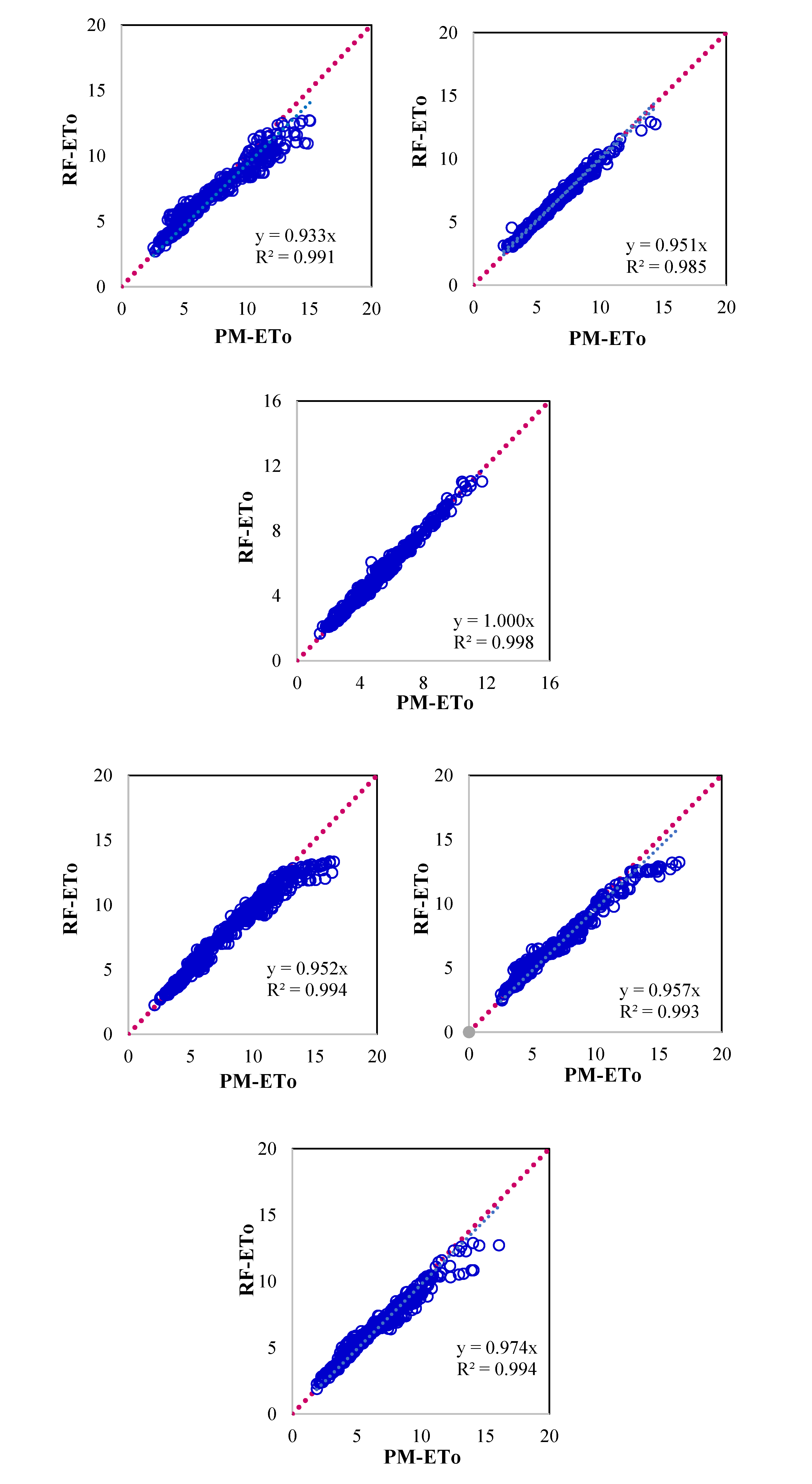
The scatter diagram of the RF model estimated ETo and PM ETo is presented in
Figure 3. For, all the locations, linear trends were observed albeit residuals are varied to some extent. The model is under estimating the higher values and over estimating the lower values. Thus, the range of model output shrinks as compare to observed values of PM ETo.
Table 3 presents the performance statistics. The model could perform fairly across the location as the WSEE values are less than 1 mm/day except Ballari and Koppal where Nash Sutcliffe model efficiency and correlation coefficient deteriorated significantly. The model performed satisfactorily on other performance criteria as well. However, the performance deteriorated significantly in predicting higher values except for locations Bengaluru, Chikmaglur, and Mandya.
3.2. Performance Evaluation of GBM Model
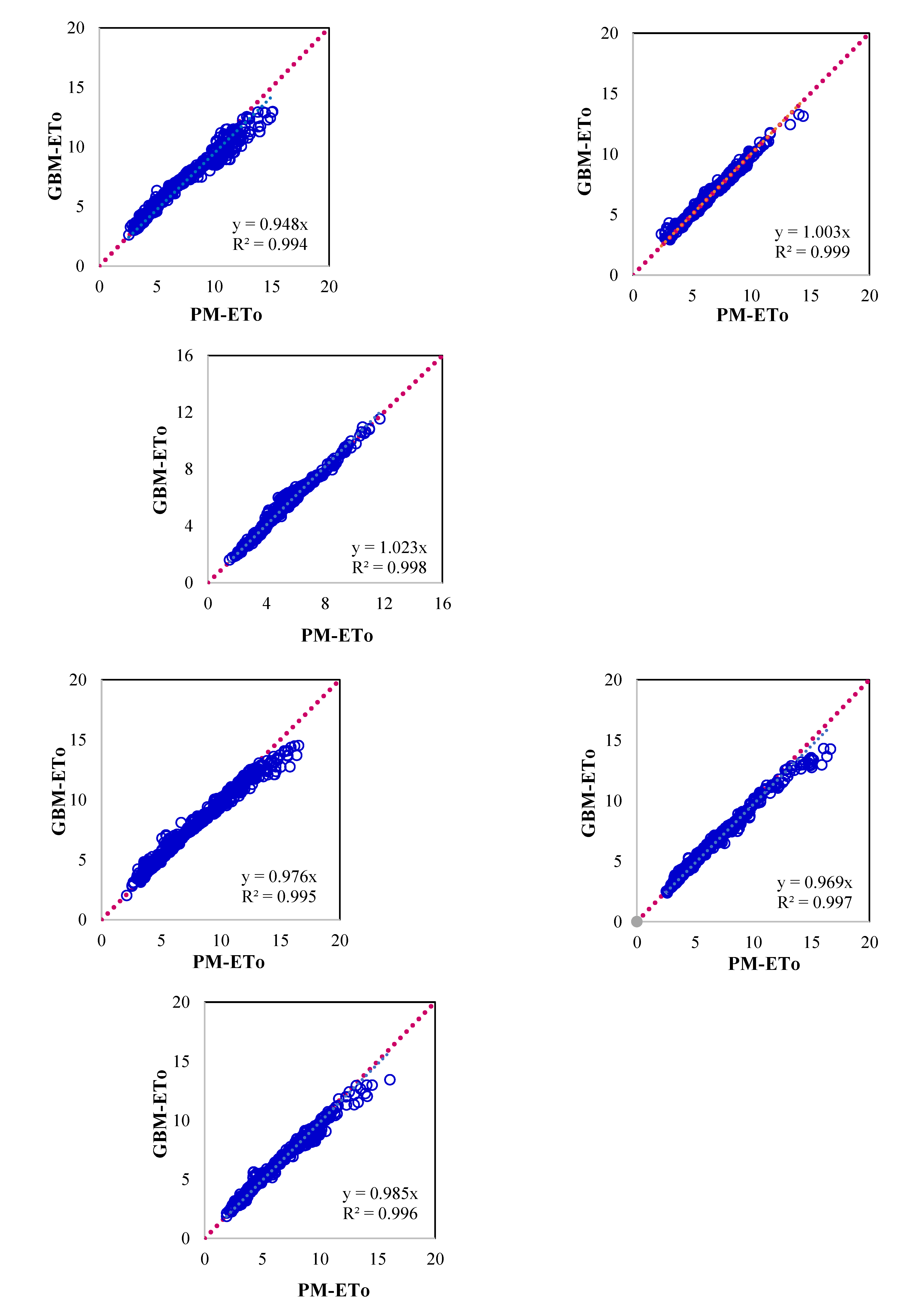
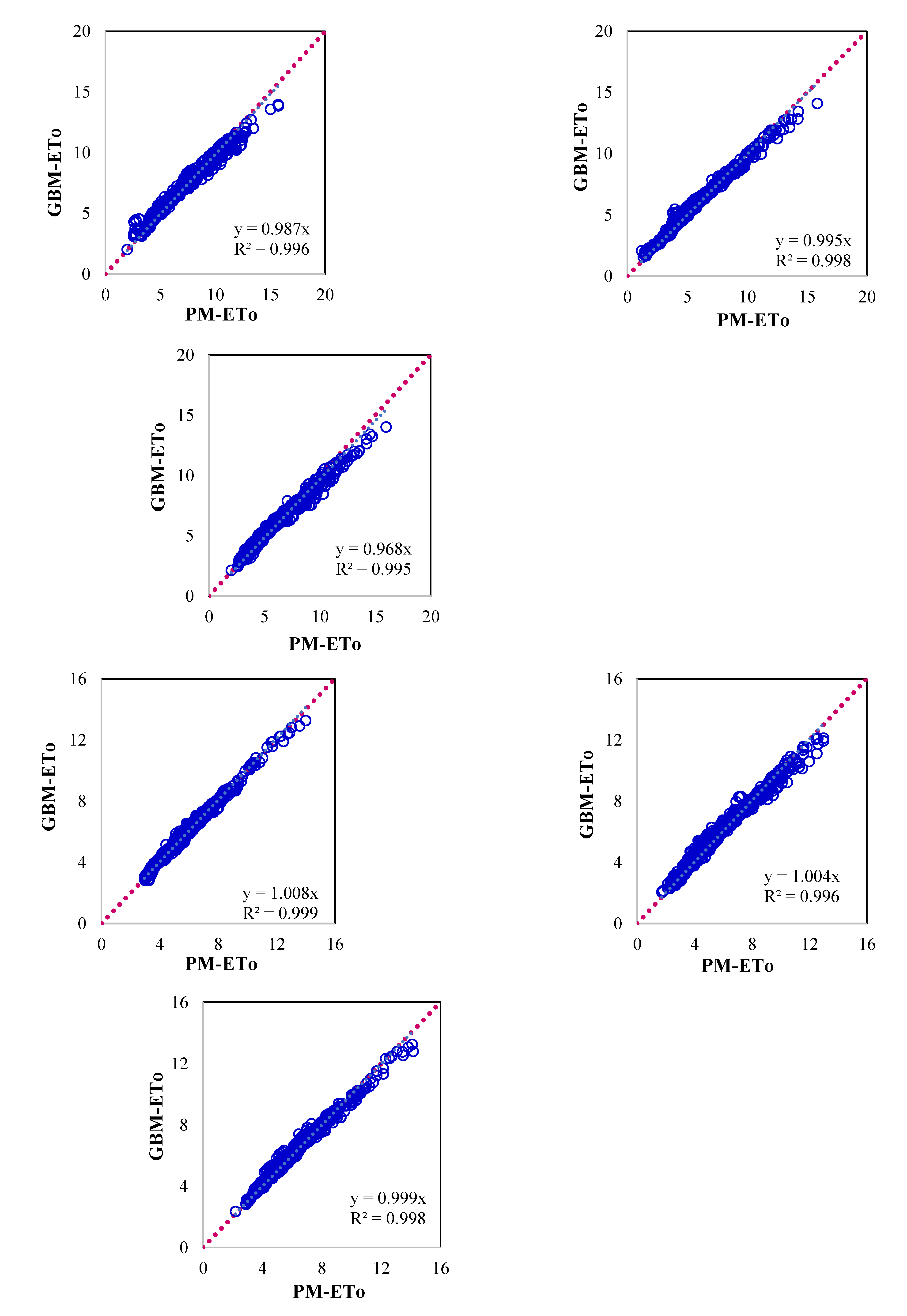
Figure 4 presents the scatter plot between P-M ETo and those estimated using the GBM model for respective locations. Significant improvement in model performance was observed as compared to the RF model for all the parameters. In this case, the WSEE error was 0.87 mm/day for all the locations as compared to 1.05 mm/day for the RF model. The limitation of the RF model is that it underestimated higher values and overestimated lower values are addressed significantly in GBM model. This model also performed substantially better than the RF model on other selected model performance criteria (
Table 4). The Nash-Sutcliffe model efficiency and correlation coefficient were more than 0.95 for all the locations. The lower noise to signal ratio indicated that the model output is less scattered and more robust as compared to the RF model.
3.3. Performance Evaluation of XGBoost Model
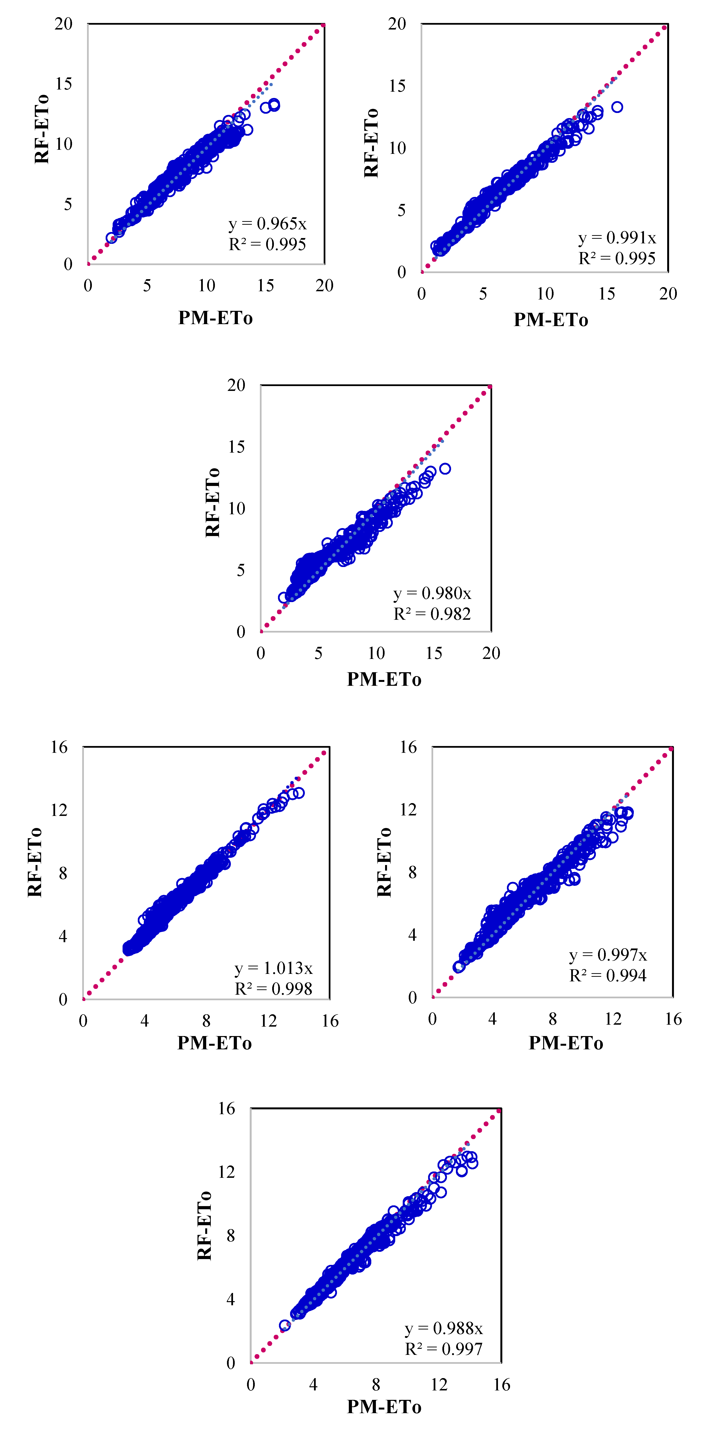
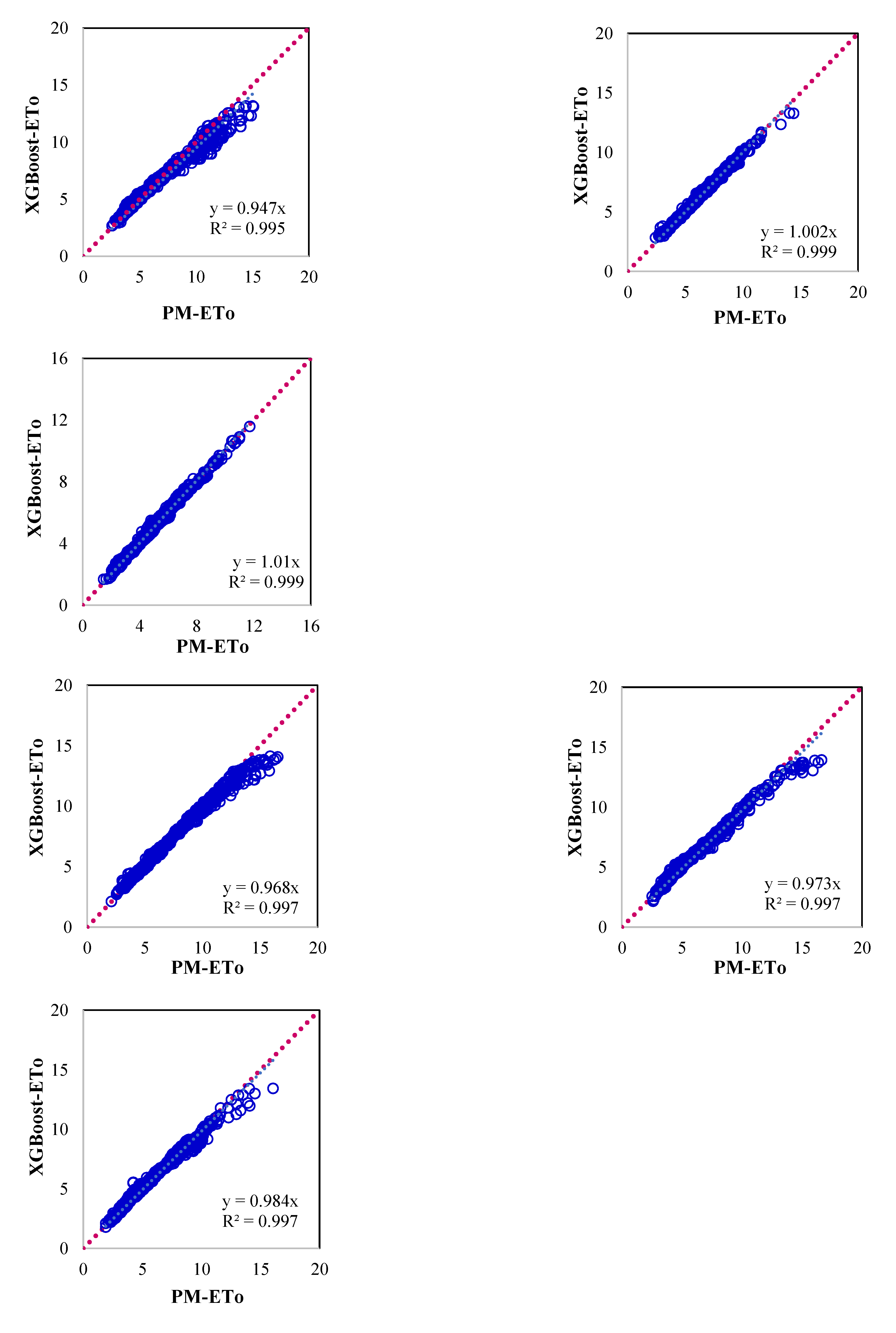
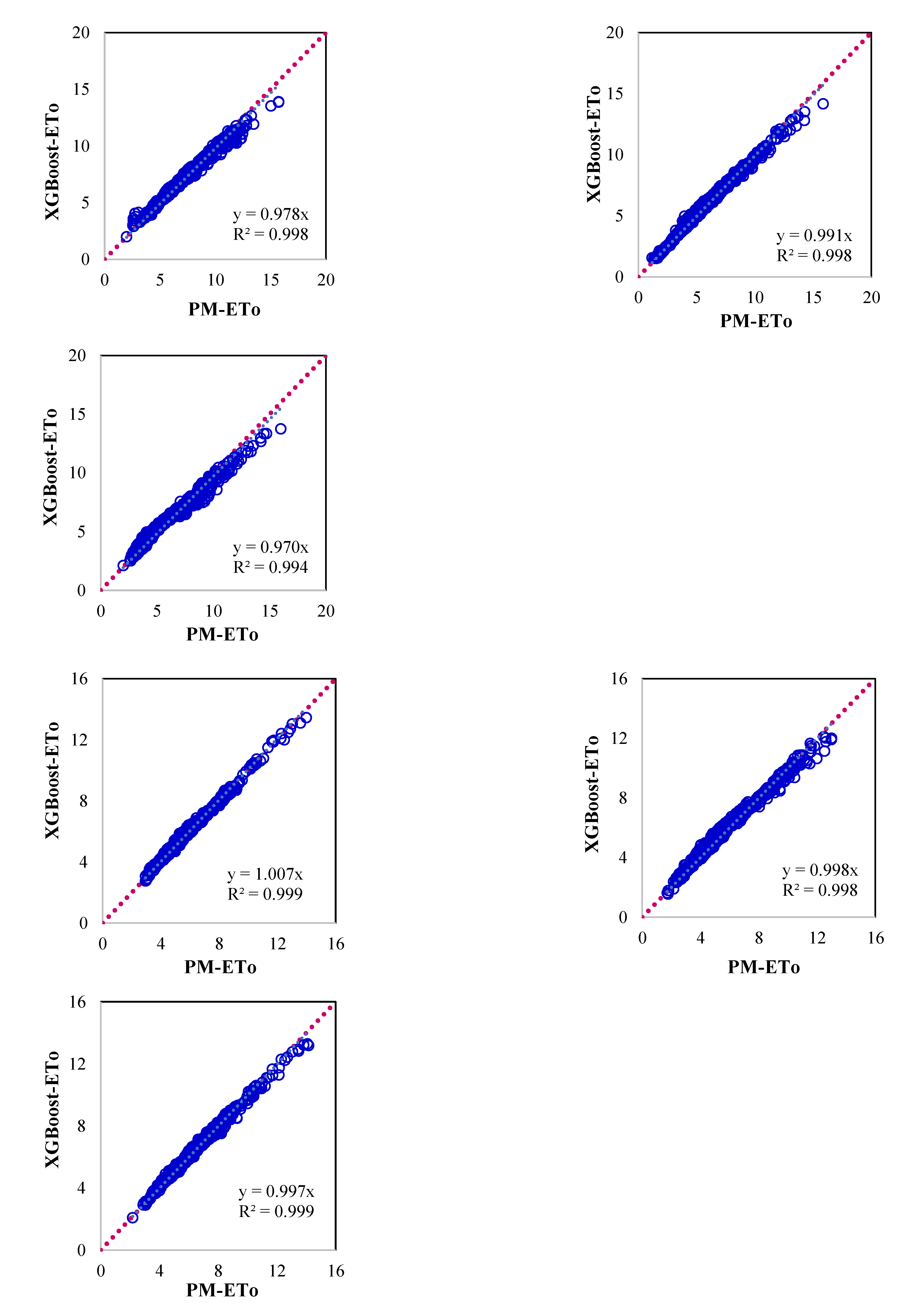
The XGBoost model further improves the performance in estimating the ETo to some extent over the GBM model. However, the improvement in model performance is significant as compared to the RF model like the case of the GBM model. In this case, lower values of NS could be obtained signifying more robustness of the model as compared to the GBM and RF model. This can be observed from the scatter plot presented in
Figure 5 which is substantiated by higher correlation coefficient and Nash-Sutcliffe model efficiency as these values are more than 0.95 (
Table 5). The WSEE in estimating PM ETo is slightly better than GBM model for all the locations as these are less than 0.85 mm/day.
4. Discussion
Over the past 20 years, there have been numerous reports in the literature about the effective use of sophisticated computer systems to estimate water requirements. On the other hand, not much has been reported on how well these computing methods generalise. All three of the chosen approaches in this study show some degree of generalisation capacity at varying degrees. Though it performs decently in the majority of locations, the more widely used RF model as a computational tool for calculating PM ETo lags noticeably behind GBM and XGBoost [
46]. Both XGBoost and GBM make use of the fastest convergence technique when operating at par. For Bengaluru, the WSEE error was, nevertheless, as low as 0.19 mm/day.
This is to be expected, as model training and validation are done using this location data. The contrary finding relates to the generalisation capacity of the GBM and XGBoost models, which fared reasonably well for sites excluded from model validation and training. The use of temporal and spatial data to map the seasonal variations, such as quarter of the year, Julian day, longitude, and latitude may be one of the factors contributing to this outstanding performance. This is particularly significant because, in contrast to the PM method, which also indirectly takes into account the temporal and spatial data, most modelling work of this kind only takes into account the basic daily climatic data of six parameters: maximum and minimum temperature, sunshine hour or solar radiation, and minimum and maximum relative humidity, and wind speed. As a result, the modelling approach’s current framework more accurately reflects the underlying evapotranspiration mechanism as specified by the PM technique.
Due to its high degree of non-linearity, the ETo at any given day is not directly correlated with the weather from the day before. With little input data, the ensemble models were able to map the underlying nonlinear evapotranspiration process. Consequently, the findings imply that these models could be used to produce estimates of PM ETo that are reasonably accurate. Moreover, the outcome can be effectively applied in other locations due to the numerical models’ capacity for generalisation. Even though daily data were used in this study, hourly data can also be used using the same methodology. The weather station might be incorporated with the XGBoost model’s produced code.
5. Conclusions
Accurate quantification of ETo is necessary for different activities such as computation of the hydrological water balance, crop water requirement, crop yield simulation, irrigation scheduling, irrigation system design, reservoir operation, and water allocation. In this study, an attempt was made to develop generalized machine learning (ML) models to estimate ETo indirectly using climatic data. For this three ensemble ML models such as XGBoost, GBM, and RF were developed using the data from one location and tested on 11 different locations without any local calibration. The findings showed that the decision tree modelling approach based on ensembled machine learning algorithms effectively takes into consideration the nonlinear link between meteorological variables and related PM ETo. The performances are further enhanced when this strategy is accompanied by an ensembled machine learning algorithm, either in the form of GBM and XGBoost boosting or RF bagging approach. For each model and location, the WSEE values produced by the three models were less than 1 mm/day for PM ETo estimation. Though all the developed ML models performed better with respect to standard PM ETo method, XGBoost model estimated ETo more accurately as compared to GBM and RF models. In this work, the ensembled machine learning technique is used to develop a mathematical model for short-term ETo estimation. This is especially crucial for real-time water management when estimating PM ETo. The "on-demand" irrigation water supply made possible by the ETo estimation, which has the potential to improve overall irrigation efficiency in the command area of large irrigation projects.
Author Contributions
Conceptualization, M.K. and Y.A.; methodology, Y.A.; software, M.K. and Y.A.; validation, M.K., Y.A. and P.; formal analysis, M.K.; investigation, Y.A.; resources, V.K.S.; data supply, A.V.M.; data curation, S.A.; writing—original draft preparation, M.K.; writing—review and editing, S.A. and A.S.; visualization, M.K.; supervision, V.K.S.; project administration, M.K.; funding acquisition, M.K. All authors have read and agreed to the published version of the manuscript.
Funding
There was no external support for this study.
Data Availability Statement
Upon request, the corresponding author will provide the data supporting the study’s findings.
Acknowledgments
The Director of the ICAR-Central Research Institute for Dryland Agriculture (CRIDA), Hyderabad, Telangana, India, is appreciated by the authors for providing the facilities required to complete the current work.
Conflicts of Interest
No conflicts of interest.
References
- Smith, M.; Allen, R.G.; Pereira, L.; Camp, C.R.; Sadler, E.J.; Yoder, R.E. Revised FAO methodology for crop water requirements. Proc., Int. Conf. on Evapotranspiration and Irrigation Scheduling, ASCE, Reston, VA, 1996, 116–123.
- Ghiat, I.; Mackey, H.R.; Al-Ansari, T. A review of evapotranspiration measurement models, techniques and methods for open and closed agricultural field applications. Water 2021, 13, 2523. [Google Scholar] [CrossRef]
- Penman, H.L. Vegetation and hydrology. Soil Sci. 1963, 96(5), 357. [Google Scholar] [CrossRef]
- Monteith, J.L. Evaporation and environment. In Symposia of the Society for Experimental Biology, 1965, 19, 205-234, Cambridge University Press (CUP) Cambridge.
- Allen, R.G.; Pereira, L.S.; Raes, D.; Smith, M. Crop evapo-transpiration: Guidelines for computing crop water requirements. Irrigation and drainage paper No. 56., 1998, FAO, Rome.
- Pereira, L.S.; Perrier, A.; Allen, R.G.; Alves, I. Evapotranspiration: Concepts and future trends. J. Irrig. Drain. Eng. 1999, 125(2), 45–51. [Google Scholar] [CrossRef]
- Jensen, M.E.; Burman, R.D.; Allen, R.G. Evapotranspiration and irrigation water requirements: A manual. ASCE manuals and reports on engineering practice (USA). 1990, No. 70, ASCE, New York.
- Srivastava, A.; Sahoo, B.; Raghuwanshi, N.S.; Singh, R. Evaluation of variable-infiltration capacity model and MODIS-terra satellite-derived grid-scale evapotranspiration estimates in a River Basin with Tropical Monsoon-Type climatology. J. Irrig. Drain. Eng. 2017, 143, 04017028. [Google Scholar] [CrossRef]
- Heramb, P.; Ramana Rao, K.V.; Subeesh, A.; Srivastava, A. Predictive modelling of reference evapotranspiration using machine learning models coupled with grey wolf optimizer. Water, 2023, 15, 856. [Google Scholar] [CrossRef]
- ASCE Task Committee on Application of Artificial Neural Networks in Hydrology. Artificial neural networks in hydrology-I: Preliminary concepts. J. Hydrol. Eng. 2000a, 5(2), 115-123.
- ASCE Task Committee on Application of Artificial Neural Networks in Hydrology. Artificial neural networks in hydrology-II: Hydrologic applications. J. Hydrol. Eng. 2000b, 5(2),124-137.
- Kumar, M.; Raghuwanshi, N.S.; Singh, R. Artificial neural networks approach in evapotranspiration modeling: A review. Irrig. Sci. 2011, 29, 11–25. [Google Scholar] [CrossRef]
- Kumar, M.; Raghuwanshi, N. S.; Singh, R.; Wallender, W.W.; Pruitt, W.O. Estimating evapotranspiration using artificial neural network. J. Irrig. Drain. Eng. 2002, 128, 224–233. [Google Scholar] [CrossRef]
- Kumar, M.; Bandyopadhyay, A.; Raghuwanshi, N.S.; Singh, R. Comparative study of conventional and artificial neural network based ETo estimation models. Irrig. Sci. 2008, 26, 531–545. [Google Scholar] [CrossRef]
- Kumar, M.; Raghuwanshi, N.S.; Singh, R. Development and validation of GANN model for evapotranspiration estimation. J. Hydrol. Eng. 2009, 14, 131–140. [Google Scholar] [CrossRef]
- Eslamian, S.S.; Gohari, S.A.; Zareian, M.J.; Firoozfar, A. Estimating Penman–Monteith reference evapotranspiration using artificial neural networks and genetic algorithm: A case study. Arab. J. Sci. Eng. 2012, 37(4), 935–944. [Google Scholar] [CrossRef]
- Adamala, S.; Raghuwanshi, N.S.; Mishra, A.; Tiwari, M.K. Evapotranspiration modeling using second-order neural networks. J. Hydrol. Eng. 2014a, 19(6), 1131–1140. [Google Scholar] [CrossRef]
- Adamala, S.; Raghuwanshi, N.S.; Mishra, A.; Tiwari, M.K. Development of generalized higher-order synaptic neural based ETo models for different agro-ecological regions in India. J. Irrig. Drain. Eng. 2014b, 140, 04014038. [Google Scholar] [CrossRef]
- Adamala, S.; Raghuwanshi, N.S.; Mishra, A. Generalized quadratic synaptic neural networks for ETo modeling. Environ. Process. 2015, 2(2), 309–329. [Google Scholar] [CrossRef]
- Dai, X.; Shi, H.; Li, Y.; Ouyang, Z.; Huo, Z. Artificial neural network models for estimating regional reference evapotranspiration based on climate factors. Hydrol. Process. 2009, 23, 442–450. [Google Scholar] [CrossRef]
- Jahanbani, H.; El-Shafie, A.H. Application of artificial neural network in estimating monthly time series reference evapotranspiration with minimum and maximum temperatures.” Paddy Water Environ. 2011, 9(2), 207–220.
- Jain, S.K.; Nayak, P.C.; Sudheer, K.P. Models for estimating evapotranspiration using artificial neural networks, and their physical interpretation. Hydrol. Process. 2008, 22, 2225–2234. [Google Scholar] [CrossRef]
- Kisi, O. The potential of different ANN techniques in evapotranspiration modelling. Hydrol. Process. 2008, 22, 2449–2460. [Google Scholar] [CrossRef]
- Kisi, O. Modeling reference evapotranspiration using evolutionary neural networks. J. Irrig. Drain. Eng. 2011a, 137, 636–643. [Google Scholar] [CrossRef]
- Kisi, O. Evapotranspiration modeling using a wavelet regression model. Irrig. Sci. 2011b, 29, 241–252. [Google Scholar]
- Marti, P.; Royuela, A.; Manzano, J.; Palau-Salvador, G. Generalization of ETo ANN models through data supplanting. J. Irrig. Drain. Eng. 2010, 136(3), 161–174. [Google Scholar] [CrossRef]
- Rahimikhoob, A. Estimation of evapotranspiration based on only air temperature data using artificial neural networks for a subtropical climate in Iran. Theor. Appl. Climatol. 2010, 101, 83–91. [Google Scholar] [CrossRef]
- Zanetti, S.S.; Sousa, E.F.; Oliveira, V.P.S.; Almeida, F.T.; Bernardo, S. Estimating evapotranspiration using artificial neural network and minimum climatological data. J. Irrig. Drain. Eng. 2007, 133, 83–89. [Google Scholar] [CrossRef]
- Yao, Y.; Liang, S.; Li, X.; Chen, J.; Liu, S.; Jia, K. ,... Roupsard, O. Improving global terrestrial evapotranspiration estimation using support vector machine by integrating three process-based algorithms. Agric. For. Meteorol. 2017, 242, 55–74. [Google Scholar] [CrossRef]
- Hassan, M.A.; Khalil, A.; Kaseb, S.; Kassem, M.A. Exploring the potential of tree-based ensemble methods in solar radiation modelling. Appl. Energy 2017, 203, 897–916. [Google Scholar] [CrossRef]
- Feng, Y.; Cui, N.; Zhao, L.; Hu, X.; Gong, D. Comparison of ELM, GANN, WNN and empirical models for estimating reference evapotranspiration in humid region of Southwest China. J. Hydrol. 2016, 536, 376–383. [Google Scholar] [CrossRef]
- Fan, J.; Wang, X.; Wu, L.; Zhou, H.; Zhang, F.; Yu, X.; Lu, X.; Xiang, Y. Comparison of Support Vector Machine and Extreme Gradient Boosting for predicting daily global solar radiation using temperature and precipitation in humid subtropical climates: A case study in China. Energy Convers. Manag. 2018, 164, 102–111. [Google Scholar] [CrossRef]
- Chia, M.Y.; Huang, Y.F.; Koo, C.H.; Fung, K.F. Recent advances in evapotranspiration estimation using artificial intelligence approaches with a focus on hybridization techniques—a review. Agronomy 2020, 10(1), 101. [Google Scholar] [CrossRef]
- Chia, M.Y.; Huang, Y.F.; Koo, C.H. Swarm-based optimization as stochastic training strategy for estimation of reference evapotranspiration using extreme learning machine. Agric. Water Manag. 2021, 243, 106447. [Google Scholar] [CrossRef]
- Tiwari, M.K.; Chatterjee, C. Development of an accurate and reliable hourly flood forecasting model using wavelet–bootstrap–ANN (WBANN) hybrid approach. J. Hydrol. 2010, 394(3-4), 458-470.
- Huang, G.; Wu, L.; Ma, X.; Zhang, W.; Fan, J.; Yu, X.; Zeng, W.; Zhou, H. Evaluation of CatBoost method for prediction of reference evapotranspiration in humid regions. J. Hydrol. 2019, 574, 1029–1041. [Google Scholar] [CrossRef]
- Ponraj, A.S.; Vigneswaran, T. Daily evapotranspiration prediction using gradient boost regression model for irrigation planning. J. Supercomput. 2020, 76(8), 5732–5744. [Google Scholar] [CrossRef]
- Wu, M.; Feng, Q.; Wen, X.; Deo, R.C.; Yin, Z.; Yang, L.; Sheng, D. Random forest predictive model development with uncertainty analysis capability for the estimation of evapotranspiration in an Arid Oasis region. Hydrol. Res. 2020a, 51(4), 648–665. [Google Scholar] [CrossRef]
- Wu, T.; Zhang, W.; Jiao, X.; Guo, W.; Hamoud, Y.A. Comparison of five boosting-based models for estimating daily reference evapotranspiration with limited meteorological variables. PLoS One 2020b, 15(6), 1–28. [Google Scholar] [CrossRef] [PubMed]
- Mokari, E.; DuBois, D.; Samani, Z.; Mohebzadeh, H.; Djaman, K. Estimation of daily reference evapotranspiration with limited climatic data using machine learning approaches across different climate zones in New Mexico. Theor. Appl. Climatol. 2022, 147(1–2), 575–587.
- Pagano, A.; Amato, F.; Ippolito, M.; De Caro, D.; Croce, D.; Motisi, A.; Provenzano, G.; Tinnirello, I. Machine learning models to predict daily actual evapotranspiration of citrus orchards under regulated deficit irrigation. Ecol. Inform. 2023, 76, 102133. [Google Scholar] [CrossRef]
- Heramb, P.; Ramana Rao, K.V.; Subeesh, A.; Srivastava, A. Predictive modelling of reference evapotranspiration using machine learning models coupled with grey wolf optimizer. Water 2023, 15(5), 1–32. [Google Scholar] [CrossRef]
- Kiraga, S.; Peters, R.T.; Molaei, B.; Evett, S.R.; Marek, G. Reference evapotranspiration estimation using genetic algorithm-optimized machine learning models and standardized Penman–Monteith equation in a highly advective environment. Water 2024, 16(1), 12. [Google Scholar] [CrossRef]
- Schonlau, M.; Zou, R.Y. The random forest algorithm for statistical learning. Stata J. Promot. Commun. Stat. Stata. 2020, 20, 3–29. [Google Scholar] [CrossRef]
- Friedman, J.H. Greedy function approximation: A gradient boosting machine. Ann. Stat. 2001, 1189–1232. [Google Scholar] [CrossRef]
- Feng, Y.; Cui, N.; Gong, D.; Zhang, Q.; Zhao, L. Evaluation of random forests and generalized regression neural networks for daily reference evapotranspiration modelling. Agric. Water Manag. 2017, 193, 163–173. [Google Scholar] [CrossRef]
Figure 1.
Map showing location locations selected for the study.
Figure 1.
Map showing location locations selected for the study.
Figure 2.
Flowchart to estimate ETo accurately using different models.
Figure 2.
Flowchart to estimate ETo accurately using different models.
Figure 3.
Scatter plot showing evapotranspiration computed by P-M method and RF Machine Learning models for (a) Ballari, (b) Bengaluru, (c) Chikmaglur, (d) Chitradurga, (e) Devanagiri, (f) Dharwad, (g) Gadag, (h) Haveri, (i) Koppal, (j) Mandya, (k) Shivmoga and (l) Tumukuru.
Figure 3.
Scatter plot showing evapotranspiration computed by P-M method and RF Machine Learning models for (a) Ballari, (b) Bengaluru, (c) Chikmaglur, (d) Chitradurga, (e) Devanagiri, (f) Dharwad, (g) Gadag, (h) Haveri, (i) Koppal, (j) Mandya, (k) Shivmoga and (l) Tumukuru.
Figure 4.
Scatter plot showing evapotranspiration computed by P-M method and GBM Machine Learning models for (a) Ballari, (b) Bengaluru, (c) Chikmaglur, (d) Chitradurga, (e) Devanagiri, (f) Dharwad, (g) Gadag, (h) Haveri, (i) Koppal, (j) Mandya, (k) Shivmoga and (l) Tumukuru.
Figure 4.
Scatter plot showing evapotranspiration computed by P-M method and GBM Machine Learning models for (a) Ballari, (b) Bengaluru, (c) Chikmaglur, (d) Chitradurga, (e) Devanagiri, (f) Dharwad, (g) Gadag, (h) Haveri, (i) Koppal, (j) Mandya, (k) Shivmoga and (l) Tumukuru.
Figure 5.
Scatter plots showing evapotranspiration computed by P-M method and XGBoost Machine Learning models for (a) Ballari, (b) Bengaluru, (c) Chikmaglur, (d) Chitradurga, (e) Devanagiri, (f) Dharwad, (g) Gadag, (h) Haveri, (i) Koppal, (j) Mandya, (k) Shivmoga and (l) Tumukuru.
Figure 5.
Scatter plots showing evapotranspiration computed by P-M method and XGBoost Machine Learning models for (a) Ballari, (b) Bengaluru, (c) Chikmaglur, (d) Chitradurga, (e) Devanagiri, (f) Dharwad, (g) Gadag, (h) Haveri, (i) Koppal, (j) Mandya, (k) Shivmoga and (l) Tumukuru.
Table 1.
Location characteristics and data.
Table 1.
Location characteristics and data.
| Sl. No. |
Location |
Location Characteristics |
Length of Records |
| Latitude |
Longitude |
Elevation |
Model Development |
Model Testing |
| 1. |
Bengaluru |
12.97 |
77.59 |
920 |
January 01, 1976 to December 31, 2017 |
January 01, 2018 to June 30, 2020 |
| 2. |
Ballari |
15.14 |
76.92 |
485 |
-- |
-do- |
| 3. |
Chikmaglur |
13.31 |
75.77 |
1090 |
-- |
-do- |
| 4. |
Chitradurga |
14.22 |
76.4 |
732 |
-- |
-do- |
| 5. |
Devnagiri |
14.33 |
75.99 |
603 |
-- |
-do- |
| 6. |
Dharwad |
15.46 |
75.01 |
750 |
-- |
-do- |
| 7. |
Gadag |
15.43 |
75.63 |
654 |
-- |
-do- |
| 8. |
Haveri |
14.79 |
75.4 |
571 |
-- |
-do- |
| 9. |
Koppal |
15.35 |
76.16 |
529 |
-- |
-do- |
| 10. |
Mandya |
12.52 |
76.89 |
678 |
-- |
-do- |
| 11. |
Shivmoga |
13.93 |
75.57 |
569 |
-- |
-do- |
| 12. |
Tumkuru |
13.34 |
77.12 |
822 |
-- |
-do- |
Table 2.
Performance criteria.
Table 2.
Performance criteria.
| Statistical model |
Equation |
| Average Absolute Relative Error |
in which,
|
| Noise to Signal Ratio |
|
| Mean Absolute Error |
|
| Coefficient of Correlation |
|
| Nash and Sutcliffe efficiency |
|
Table 3.
Model performance on various criteria of the RF model.
Table 3.
Model performance on various criteria of the RF model.
| Location |
Model Performance Criteria |
| WSEE |
r |
AARE |
NS |
MAE |
ɳ |
| Ballari |
1.05 |
0.92 |
7.36 |
0.26 |
0.56 |
0.92 |
| Bengaluru |
0.28 |
0.98 |
3.24 |
0.13 |
0.19 |
0.98 |
| Chikmaglur |
0.33 |
0.98 |
3.60 |
0.12 |
0.16 |
0.99 |
| Chitradurga |
0.99 |
0.96 |
5.14 |
0.21 |
0.45 |
0.95 |
| Devnagiri |
0.74 |
0.95 |
6.45 |
0.20 |
0.41 |
0.95 |
| Dharwad |
0.72 |
0.94 |
6.04 |
0.21 |
0.36 |
0.95 |
| Gadag |
0.88 |
0.93 |
5.75 |
0.24 |
0.44 |
0.94 |
| Haveri |
0.56 |
0.96 |
6.34 |
0.18 |
0.34 |
0.97 |
| Koppal |
1.00 |
0.80 |
13.05 |
0.32 |
0.68 |
0.89 |
| Mandya |
0.31 |
0.98 |
3.73 |
0.15 |
0.21 |
0.98 |
| Shivmoga |
0.55 |
0.94 |
6.66 |
0.21 |
0.36 |
0.96 |
| Tumkuru |
0.39 |
0.97 |
3.78 |
0.16 |
0.25 |
0.97 |
Table 4.
Model performance on various criteria of the GBM model.
Table 4.
Model performance on various criteria of the GBM model.
| Location |
Model Performance Criteria |
| WSEE |
r |
AARE |
NS |
MAE |
ɳ |
| Ballari |
0.87 |
0.95 |
5.43 |
0.21 |
0.43 |
0.95 |
| Bengaluru |
0.25 |
0.98 |
3.14 |
0.12 |
0.17 |
0.98 |
| Chikmaglur |
0.32 |
0.98 |
3.75 |
0.15 |
0.18 |
0.98 |
| Chitradurga |
0.76 |
0.96 |
5.70 |
0.21 |
0.45 |
0.95 |
| Devnagiri |
0.53 |
0.98 |
4.00 |
0.14 |
0.27 |
0.98 |
| Dharwad |
0.56 |
0.97 |
4.74 |
0.16 |
0.27 |
0.97 |
| Gadag |
0.66 |
0.95 |
5.14 |
0.19 |
0.34 |
0.96 |
| Haveri |
0.39 |
0.98 |
4.41 |
0.10 |
0.19 |
0.99 |
| Koppal |
0.61 |
0.96 |
5.38 |
0.17 |
0.33 |
0.96 |
| Mandya |
0.21 |
0.99 |
2.84 |
0.11 |
0.15 |
0.99 |
| Shivmoga |
0.42 |
0.97 |
5.63 |
0.16 |
0.29 |
0.97 |
| Tumkuru |
0.31 |
0.98 |
3.28 |
0.14 |
0.20 |
0.98 |
Table 5.
Model performance on various criteria for EML-XGBoost.
Table 5.
Model performance on various criteria for EML-XGBoost.
| Location |
Model Performance Criteria |
| WSEE |
r |
AARE |
NS |
MAE |
ɳ |
| Ballari |
0.84 |
0.96 |
4.91 |
0.20 |
0.40 |
0.95 |
| Bengaluru |
0.19 |
0.99 |
2.13 |
0.09 |
0.12 |
0.99 |
| Chikmaglur |
0.19 |
0.99 |
2.82 |
0.09 |
0.13 |
0.99 |
| Chitradurga |
0.71 |
0.98 |
3.43 |
0.15 |
0.29 |
0.98 |
| Devnagiri |
0.49 |
0.98 |
3.77 |
0.13 |
0.25 |
0.98 |
| Dharwad |
0.50 |
0.98 |
3.89 |
0.14 |
0.23 |
0.98 |
| Gadag |
0.62 |
0.97 |
3.80 |
0.16 |
0.27 |
0.97 |
| Haveri |
0.33 |
0.99 |
3.17 |
0.10 |
0.19 |
0.99 |
| Koppal |
0.66 |
0.95 |
6.11 |
0.18 |
0.36 |
0.96 |
| Mandya |
0.19 |
0.99 |
2.43 |
0.09 |
0.13 |
0.99 |
| Shivmoga |
0.34 |
0.98 |
4.18 |
0.13 |
0.23 |
0.98 |
| Tumkuru |
0.22 |
0.99 |
2.35 |
0.09 |
0.15 |
0.99 |
|
Disclaimer/Publisher’s Note: The statements, opinions and data contained in all publications are solely those of the individual author(s) and contributor(s) and not of MDPI and/or the editor(s). MDPI and/or the editor(s) disclaim responsibility for any injury to people or property resulting from any ideas, methods, instructions or products referred to in the content. |
© 2024 by the authors. Licensee MDPI, Basel, Switzerland. This article is an open access article distributed under the terms and conditions of the Creative Commons Attribution (CC BY) license (http://creativecommons.org/licenses/by/4.0/).
