1. Introduction
In recent years, complex networks have been widely studied because of its important applications in reality. It is a special mathematical model that considers the relationships between objects in the real world. Moreover, it generally has three properties: (1) The small world property [
1], which describes the shortest distance between any two nodes on the network is short. (2) Scale-free property [
2,
3], where the degree distribution of nodes conforms to a power rate distribution, i.e., most of the nodes have smaller degree and very few nodes have larger degree. (3) Community structure [
4,
5], i.e., the nodes on the network exhibit the characteristics of clusters. It is a subgraph structure with tight internal connections and sparse external connections. Most networks are characterized with community structure. For example, communities in the social network [
6,
7] represent closely related groups. Communities in the citation network [
8] represent clusters of articles in a particular field of study. Communities in the protein-to-protein interaction network [
9] represent clusters of proteins with similar biological functions. Therefore, community detection is gradually becoming an important research area in complex networks.
Some community detection algorithms based on random walk [
10,
11] need to set a convergence condition and end the random walk when this condition is satisfied, which may spend a longer time. The label propagation algorithm (LPA) [
12] has a disadvantage in detecting communities, i.e., the randomness of label propagation. It may detect poor quality communities. The proposed algorithm uses random walk and the label propagation while addressing its disadvantages.
In this paper, a random walk algorithm based on different seed nodes to detect communities is proposed, named RWBS. A new metric is proposed to measure the importance of nodes, we can get the similarity between any two nodes on the network by this metric. Based on , we propose two algorithms that are suitable for different types of networks to obtain seed nodes of the random walk. Moreover, RWBS changes the transfer probability matrix to get better information about the network. According to the six degrees of separation theory in complex networks, the steps of random walk is set to 6, which not only can shorten the time of the random walk, but also can obtain the structural information of the network. After calculating the weight of the edge, the new label propagation rule is used to propagate the label, and the initial community structure is obtained based on the convergent label. Finally, the modularity (Q) is chosen as the optimization function to further combine communities and improve communities quality. Experiments on real-world and synthetic networks demonstrate the effectiveness and superiority of RWBS. The following are the main innovations of paper.
We propose a random walk algorithm based on different seed nodes to detect communities, named RWBS.
We propose a new centrality metric () for measuring the importance of nodes that combines degree centrality () and closeness centrality () and performs better than () and ().
Two algorithms are proposed to obtain seed nodes for different networks.
Experimental results on real-world and synthetic networks show that the RWBS algorithm can be effective in finding communities.
2. Related Works
With the intensive study of community structure in complex networks, more and more effective community detection algorithms have been proposed. Below, we describe each of these methods.
2.1. The Traditional Methods
The Traditional methods can be meticulously classified into the following three methods.
The partitional clustering method: The method is to divide the network into
K subgraphs of predefined size such that the edges within each subgraph are denser and the edges between different subgraphs are sparser. Commonly used algorithms are KL algorithm [
13] and spectral bisection algorithm [
14]. The disadvantage of this class of methods is that the size of the community needs to be set in advance. However, real-world networks are largely unknown about their community structure, making it difficult to apply it in practice.
The hierarchical clustering methods: Networks can be represented by adjacency matrices or small matrices after dimensionality reduction such as matrix factorization transformation, and then clustered using conventional clustering algorithms. The first method is the hierarchical clustering approach, which considers a graph to be a large community that contains a complex topology, i.e., the community may be a collection of smaller communities of different sizes [
15]. Another method is that of spectral clustering, which consists of the method of using matrix eigenvectors and the method of classifying nodes based on pairwise similarities between data points [
16]. In 2022, Ullah et al. proposed an Information Interaction Model, named RIIM algorithm [
17].
The divisive method: This method obtains the community structure by calculating the similarity of edges to remove edges with lower similarity [
18]. The entire network is first categorized into a community, and then the edges connecting the low-similarity vertices and the highest edge interdimensionality are removed. The method is a top-down hierarchical clustering algorithm. For example, the time complexity of the GN algorithm [
5] proposed by Girvan and Newman in 2002 is
. The disadvantage of this algorithm is the high time complexity, which makes it difficult to be applied to large networks.
2.2. The Modularity-Based Methods
Modularity [
19] can be used to measure the quality of the community. A higher value of modularity also means that the quality of the community obtained is better. Many scholars have used the modularity as the optimization function to achieve the optimal division result when dividing communities.
Greedy optimization: In 2004, Newman [
20] proposed a greedy method for maximizing modularity, which was an aggregation technique. Its time complexity on the sparse graph is
. Another greedy optimization algorithm is an algorithm called Louvain (BGLL) [
21] proposed by Blondel et al. Its time complexity is
.
Simulated annealing: It is a globally optimized discrete stochastic method to detect communities in complex networks by maximizing the modularity. For example, Guimerà and Amaral [
22] proposed an annealing modularity optimization algorithm (SA) based on the principle of simulated annealing algorithm.
Extremal optimization: In 2001, Boettcher [
23] et al. proposed extremal optimization as a general heuristic search technique for physical and combinatorial optimization problems. In 2005, Duch et al. [
24] used it for modularity optimization to detect communities.
Genetic algorithms: Genetic algorithms are optimization techniques inspired by biological evolution. They can also be used to optimize the modularity to detect communities. For example, in 2018, M’Barek [
25] et al. proposed a Genetic Algorithm (GA) based approach to find communities in a gene interaction network. In 2019, a new matrix-based genetic algorithm for community detection was proposed by Chen and Bi, named MGA algorithm [
26].
Evolutionary algorithms: It is a type of metaheuristic optimization algorithm based on artificial intelligence. Their effectiveness in local learning and global search is well known. For example, in 2021, Pourabbasi et al. proposed a single-chromosome evolutionary algorithm combining content and structural information to detect communities [
27]. Su et al. proposed a parallel multi-objective evolutionary algorithm, called PMOEA [
28].
2.3. The Dynamic Community Detection Methods
We introduce three dynamic community detection methods.
Algorithms based on random walk: In the process of random walk, the random walker starts walking within the community from one node and randomly moves to the neighboring nodes at each step. The random walker spends a long time in the dense community because of the dense edge connections within the community. The algorithms based on random walk are PageRank algorithm [
29], Walktrap [
10], and Infomap [
30].
Algorithms based on LPA [
12]: The LPA algorithm is widely used to find communities in large networks due to its advantages of lower time complexity and space complexity. The detailed steps of LPA are shown in
Section 3.4. Since the LPA algorithm has the advantage of low time complexity, many scholars have researched and proposed many LPA-based community division algorithms based on this algorithm. For example, SLPA [
31], LPA_CL [
32], VLPA [
33], etc..
Other algorithms: There are a few other dynamic community division algorithms. For example, the CDME algorithm that is based on the Matthew effect [
34], The GBTM algorithm for community detection in dynamic networks by Hidden Markov Method [
35].
3. Preparation of Algorithm
3.1. The Definition of Symbols
The community division algorithm proposed in this paper is proposed for undirected and unweighted networks. Therefore, all the datasets used in this paper are undirected and unweighted networks. We assume that the network is
G. The set of nodes and edges of the network can be defined as
and
, respectively. Then,
G can be expressed by
and
, i.e.,
. The definitions of other mathematical symbols used in this paper are shown in
Table 1.
3.2. Evaluation Metrics
We use Normalized Mutual Information (
) [
36], Adjusted Rand Index (
), and Modularity (
Q) [
19] as the evaluation metrics to measure the quality of communities. Let
and
represent the detected community by the proposed algorithm and the real community of the network, respectively. All three metrics are such that a larger value represents a better quality community obtained. The specific descriptions of these metrics are shown below.
-
[
36]: Where
is used to measure the similarity of the communities detected by our proposed algorithm with the real communities of the network. The definition of
is shown below.
and are the entropies of X and Y. represents the mutual information between X and Y.
-
[
37]: Similarly,
is used to measure the similarity of the communities detected by our proposed algorithm with the real communities of the network. It is defined as Eq. (2).
Where , , and (, ).
-
Q [
19,
38]: The modularity is defined as follows:
Where represents the community to which node i belongs. The network G can be described by the adjacency matrix , if and 0 otherwise. is 1 if and 0 otherwise.
3.3. The Importance of Nodes
Measuring the importance of nodes is also an important issue in the field of complex networks and has a wide variety of applications. Some centralities are important metrics for measuring the importance of nodes. For example, degree centrality [
39], betweenness centrality [
40], closeness centrality [
41], eigenvector centrality [
42], pagerank centrality [
43], etc. The centralities used in this paper are described below.
3.3.1. Degree Centrality
Degree centrality [
39] measures the importance of a node by its degree. Higher degree of a node means that the node is more important. It is defined as Eq. (4).
However, the above definition does not take into account the size of the network. To solve this problem, Stanley Wasserman and Katherine Faust [
44] proposed the standardized degree centrality. It can be described as:
3.3.2. Closeness Centrality
This centrality [
41] can reflect the closeness between two nodes. It is defined as follows:
where
represents the shortest distance between node
i and node
j. When the sum of the shortest distances from node
i to other nodes on the network is shorter, then its closeness centrality is higher.
3.3.3. Mixed Centrality
To fully combine both of these centrality, we introduce the mixed centrality.
is defined as Eq. (7).
We test the effectiveness of the mixed centrality. Network efficiency reflects how well-connected the network is. As a general rule, the better the network connection, the more efficient the network [
45]. The following is its definition.
Then, we observe the decline rate of network efficiency by deleting node
i as a way to determine whether the node’s importance ranking in the network is justified. Let
be the decline rate of network efficiency:
where
is the efficiency of the network after removing node
i and
is the original efficiency of the network. The larger
is, the more important the removed node
i is. It should occur with a clear correlation between the decline rate of network efficiency and the importance of a node as the importance of a node decreases. As an explanation of the decline rate of network efficiency when the node is removed,
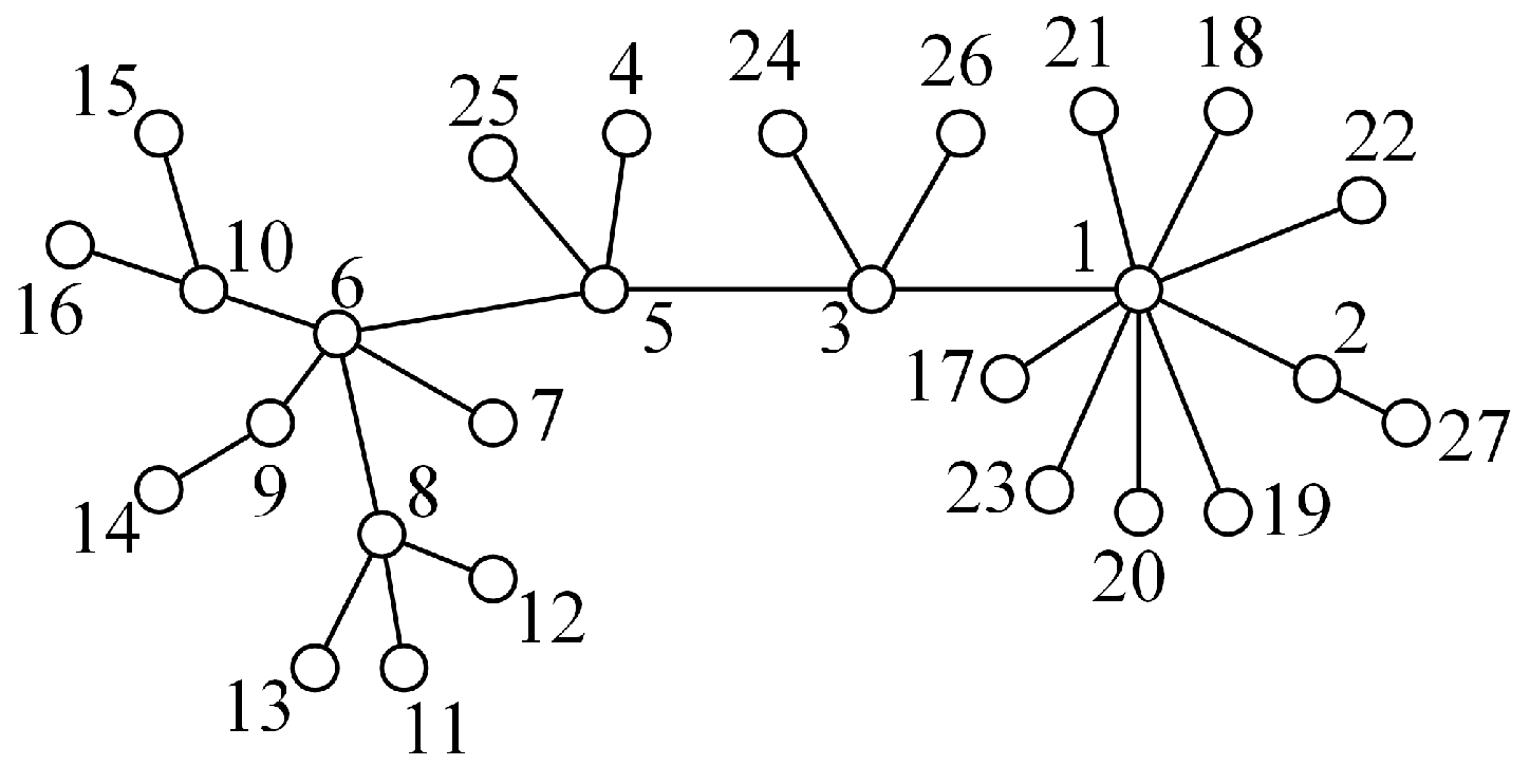
Figure 1 is shown.
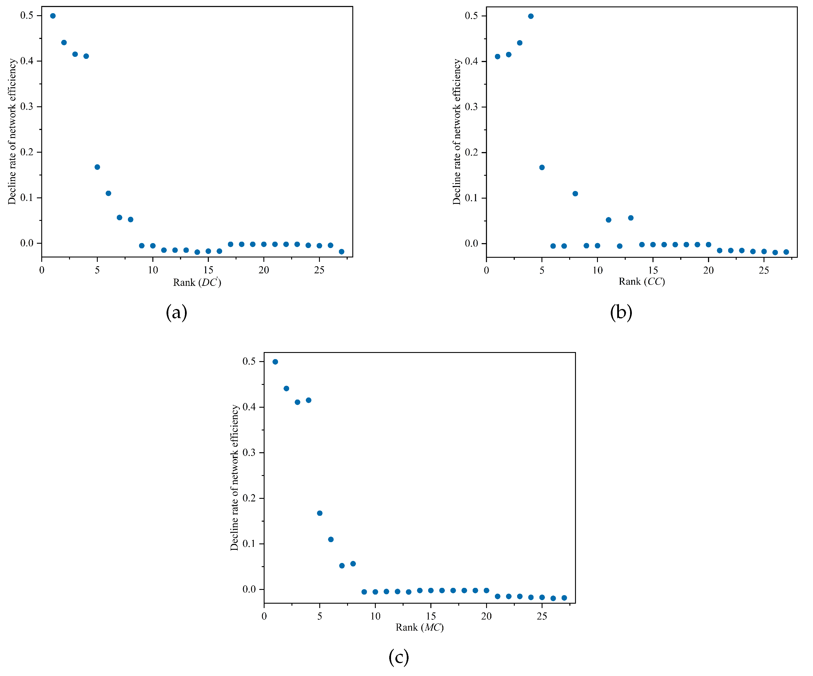
Figure 2 shows the correlation between the decline rate of network efficiency and the importance of nodes ranked by
,
, and
. From
Figure 2(c), it can be seen that overall the rate of decrease in network efficiency decreases as the
value of the deleted node decreases. It is clear that the decline rate of the network efficiency correlates with the importance of the node for
and
methods, and
performs better. The performance of
is the worst, and in
Figure 2(b), the decline rate of the network efficiency and the importance of the node do not appear to be correlated. Therefore, we propose
as an effective metric to measure the importance of nodes.
3.4. LPA Algorithm
First, we introduce the process of the LPA algorithm [
12].
Step 1: We assign a label to each node in the network and the labels are different for different nodes, i.e., , and if , then ().
Step 2: Randomly select node i from and update the label of this node according to the following rule: Node i selects one of the most frequently occurring labels from the labels of its neighboring nodes as the new label of node i. If the label with the most frequent occurrence is not unique, one is chosen randomly.
Step 3: The algorithm stops when the labels of all nodes are no further updated.
In Step 2, when the node randomly selects labels it may be the case that a wrong label selection in one step leads to wrong label selection in each of the following steps. Poor quality communities may eventually be detected. In section 4.1.2, we will introduce a new rule to address this shortcoming.
4. The Proposed Algorithm (RWBS)
4.1. The Detailed Steps of Algorithm
The proposed algorithm (RWBS) consists of three main steps: random walk based on different seed nodes, propagation of labels and combination of communities. We explain these three steps in details below.
4.1.1. Random Walk Based on Different Seed Nodes
Let the transfer probability matrix is
. In general, the probability of node
i jumping to its neighboring nodes is the same, i.e.,
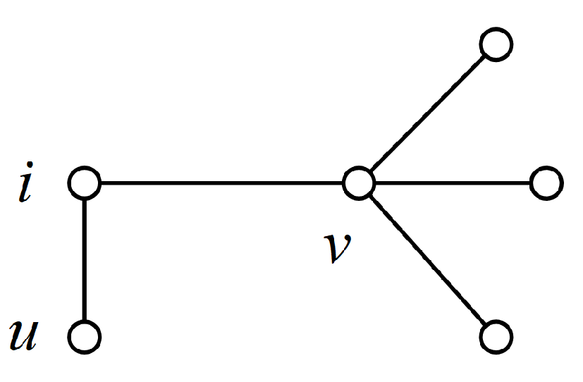
. For example, in
Figure 3, node
i has the same probability of selecting node
u and node
v as the node for the next jump. But the proposed algorithm changes the transfer rule of node
i. We consider that nodes with larger degree have higher probability to attract node
i, i.e., node
i has higher possibility to transfer to node
v in
Figure 3 (
).
is defined as Eq. (10).
After the random walk algorithm is ended, the random walker prefers to stay at nodes with large degree. If the node with large degree is chosen as the initial node for random walk, there is no doubt that the random walker will stay at the node with large degree when the random walk stops. It will result that the information of the nodes with small degree will be ignored. Then, a new rule for the selection of initial nodes is proposed. To better obtain the structure of the network, we consider the distance between the nodes when selecting the initial nodes. The selected nodes with small mixed centrality tend to be located at the fringe of the network. Thus, when the selected seed nodes have the larger distance between them and have the small mixed centrality, the random walker can walk faster to the center nodes, and the structure of the network can be obtained faster. To select seed nodes with the above characteristics, we define the attraction between nodes
, which considers the mixed centrality of nodes and
.
After obtaining the attraction
between any two nodes, we select the set of seed nodes
S. For networks with ground-truth, we set the number of seed nodes is the number of communities, i.e.
c. Let
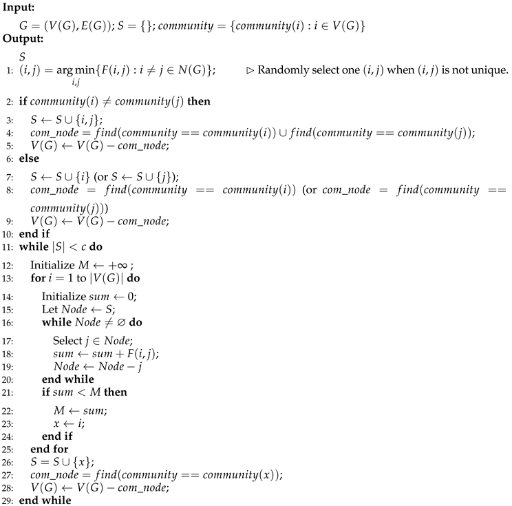
, which store the name of the community to which each node on the network belongs. The pseudo-code for selecting specific seed nodes is shown in Algorithm 1. For networks without ground-truth, we set the number of seed nodes is
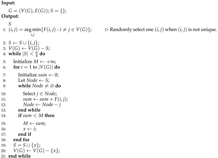
, and the pseudo-code for selecting specific seed nodes is shown in Algorithm 2.
|
Algorithm 1 Select seed nodes on the network with ground-truth. |
 |
Let
denote the probability that the random walker stays at each node in the initial state, and the
i-th (
) element of
is
. The proposed algorithm lets the random walker start from the seed nodes (
S) in the initial state, and if the degree of the node is larger, the probability of starting from that node is higher. It is shown in Eq. (12).
We use the random walk with restart algorithm (RWR) [
46], which is a modification of the random walk algorithm. The algorithm faces two options at each step of the walk, the first option is to jump randomly to the neighbor node of the current node, and the other option is to return to the initial node, i.e.,
S. It contains a parameter
, which indicates the restart probability. When the number of random walk steps
t is too large, the random walker prefers to stay at the node with large degree. The six degrees of separation theory states that the path length between any two people in the social network is short. That is, everyone in the social network can reach out to others in about six steps or less [
47]. Thus, let the random walker stop after walking 6 steps, i.e.,
.
In this paper, let
. We can obtain the probability
that the random walker stays at each node after the end of the random walk algorithm.
|
Algorithm 2 Select seed nodes on the network without ground-truth. |
 |
4.1.2. Propagation of Labels
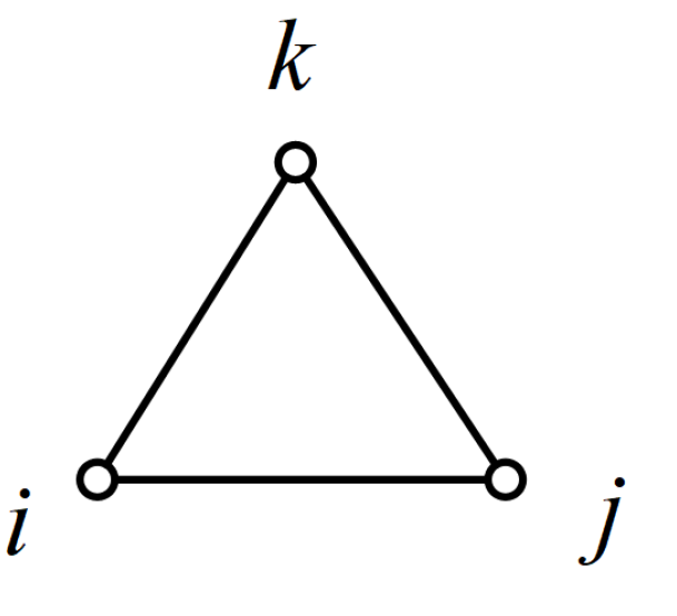
In this model we also consider the triangular to measure the closeness between node pairs. Its specific structure is shown in
Figure 4. If node
i and node
j have a common neighbor node
k, the triangle is formed between
, which indicates that they have a close relationship. We measure the closeness between node
i and node
j by the number of neighbor nodes between them. The number of triangles can be expressed by Eq. (14).
where
denotes the number of triangular structures formed by node
i and node
j. The closeness
between node
i and node
j can be expressed by Eq. (15).
For the label propagation in the next, we add a weight
to edge
(
), which considers the closeness between node
i and node
j and the probability of staying at node
i and node
j.
can be defined by Eq. (16).
Before performing label propagation, we assign a label to each node. The set of labels of nodes is set to
, and
when
. The label of the current node is updated according to the labels of its neighboring nodes in turn, and the label update rule is shown below.
where
denotes the new label of node
i. When there exists more than one node
j such that
has a maximum value, then
randomly selects one from the labels of these nodes. The algorithm stops when the labels of all nodes are no further updated. Let the final community as
. Where each node in
(
) has the same label. The label propagation rule in Eq. (17) solve the shortcoming of LPA mentioned in
Section 3.4.
4.1.3. Combination of Communities
To improve the quality of the detected communities, we use
Q as the optimization function to combine communities. Take any two different communities from
and the rule of combining communities is shown in Eq. (18).
where
, and
represents the modularity before (after) combining communities.
4.2. Time Complexity
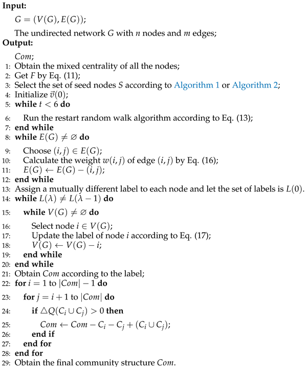
The pseudo-code of RWBS is shown in Algorithm 3.
Obtain the mixed centrality of nodes on the network, and its time complexity is
. Next, calculate the similarity
between any two nodes on the network, which has the time complexity
. The seed nodes of random walk are obtained by Algorithm 1 or Algorithm 2. For networks with ground-truth, the time complexity of Algorithm 1 is
. For networks without ground-truth, the time complexity of Algorithm 2 is
. The time complexity of obtaining the probability vector
after
t steps is
[
10]. In this paper, the random walker is set to walk 6 steps on the network, so the time complexity of the process is
. Assume that the label propagation requires
h iterations to converge. The time complexity of the label propagation is
. After the end of label propagation, assume that
c communities are obtained. The time complexity of combining any two communities is
. In summary, for networks with ground-truth, the total time complexity of the RWBS algorithm is
. For networks without ground-truth, the total time complexity of the RWBS algorithm is
. So the time complexity of the RWBS algorithm is
.
|
Algorithm 3 RWBS |
 |
4.3. A Simple Example
To explain the RWBS algorithm in details, we give an sample network to illustrate how it detects communities. The sample network is shown in
Figure 5(a), which contains 9 nodes and 15 edges.
Figure 5(b) shows the real community structure of this sample network, which contains two communities
and
. The degree, closeness, and mixed centrality of the nodes are calculated, and the results are shown in
Table 2.
First, the transfer probability matrix
P can be obtained by Eq. (10), and it is shown in Eq. (19).
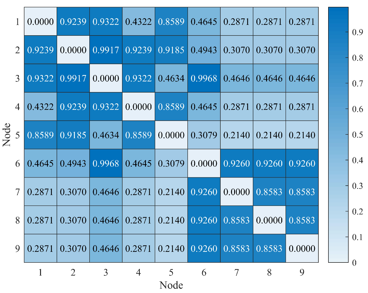
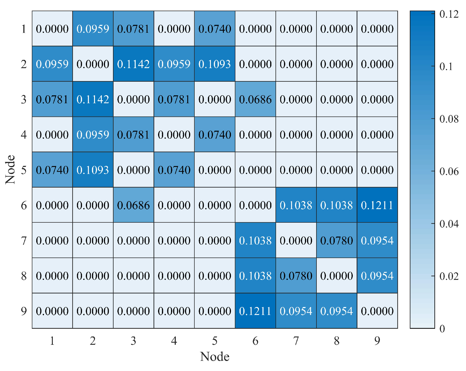
The similarity between nodes can be calculated by Eq. (11), and it is shown in
Figure 6. Because the sample network contains two communities, let the number of seed nodes is 2, and obtain the specific seed nodes by Algorithm 1. From
Figure 6, the similarity between node 5 and nodes 7, 8, 9 all have minimum value, node 5 can be selected as seed node. Moreover, we randomly select node 9 between 7, 8, 9 as seed node. Finally,
.
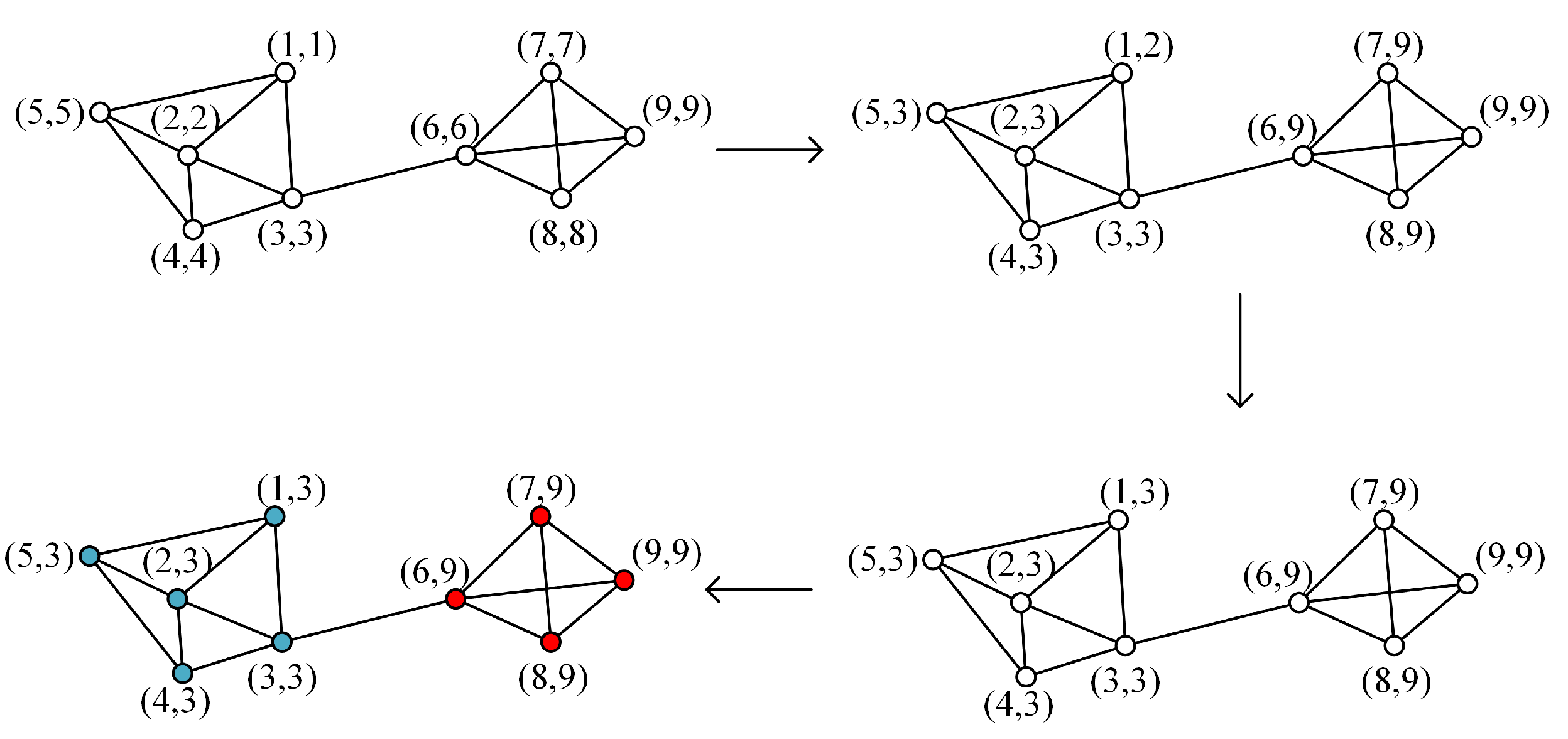
We assign a data pair
to each node.
denotes the name of the node. Let
.
and
w can be obtained when the algorithm ends (Four decimal places of
are retained). Where
, and
w is shown in
Figure 7. The label propagation process is shown in
Figure 8. From
Figure 8, the sample network contains two communities (
and
), which is consistent with the real community structure of this network. The modularity
Q of this situation is 0.4244. If
and
are combined into one community, then
. Thus,
and
are the final community structure.
5. Experiments
To evaluate the performance of RWBS algorithm in finding communities, we conducted experiments on the real-world and synthetic networks, respectively. For both the real-world networks with-ground truth and the synthetic networks, the community structure of these networks is already known, and are used to measure the similarity between the communities detected by RWBS and the real community structure. Higher values of these metrics indicate better quality of communities. For real-world networks without ground truth, the modularity (Q) is used to measure the quality of the detected communities, since we are not sure about the community structure of such networks.
5.1. Experiment on Real-World Networks
The following seven different real-world networks are chosen. The Karate, Dolphin, Political, and Football networks are networks with ground-truth. The Last, PGP, and Email networks are networks without ground-truth. In
Table 3, we give information about these networks.
Karate network [
48]: It is a social network with 34 members and 78 member relationships constructed by Zachary by observing the social relationships between members of a karate club at a university in the USA. Two members are considered to have edges to each other if they are frequently seen together in settings other than club activities. The club split into 2 smaller clubs with their own core because of a dispute between the director and the coach.
Dolphin network [
49]: In 2003, Lusseau et al. observed the habits of 62 broad-snouted dolphins, and they found that these dolphins showed specific patterns of interactions and constructed a social network containing 62 nodes. If two dolphins are frequently active together, an edge exists between the two corresponding nodes in the network.
Political network [
50]: The network is built by Krebs from pages of American politics-related books sold on Amazon. Its nodes represent American politics-related books, and edges represent a certain number of readers who have purchased both books. The nodes on the network are categorized as "liberal", "conservative" and "centrist". These divisions were manually analyzed by Newman based on the views and ratings of books on Amazon.
Football network [
5]: The network shows games played in the American College Football League. The nodes in the network represent 115 teams, and edges represent two teams that have played a game against each other.
Last network [
51]: This is a network based on the friendship between Last.fm users in Finland.
PGP network [
52]: The network is an undirected network of bidirectional trust connections where each node contains both public and private keys.
Email network [
53]: The network is built on the basis of relationships between users who email each other.
and
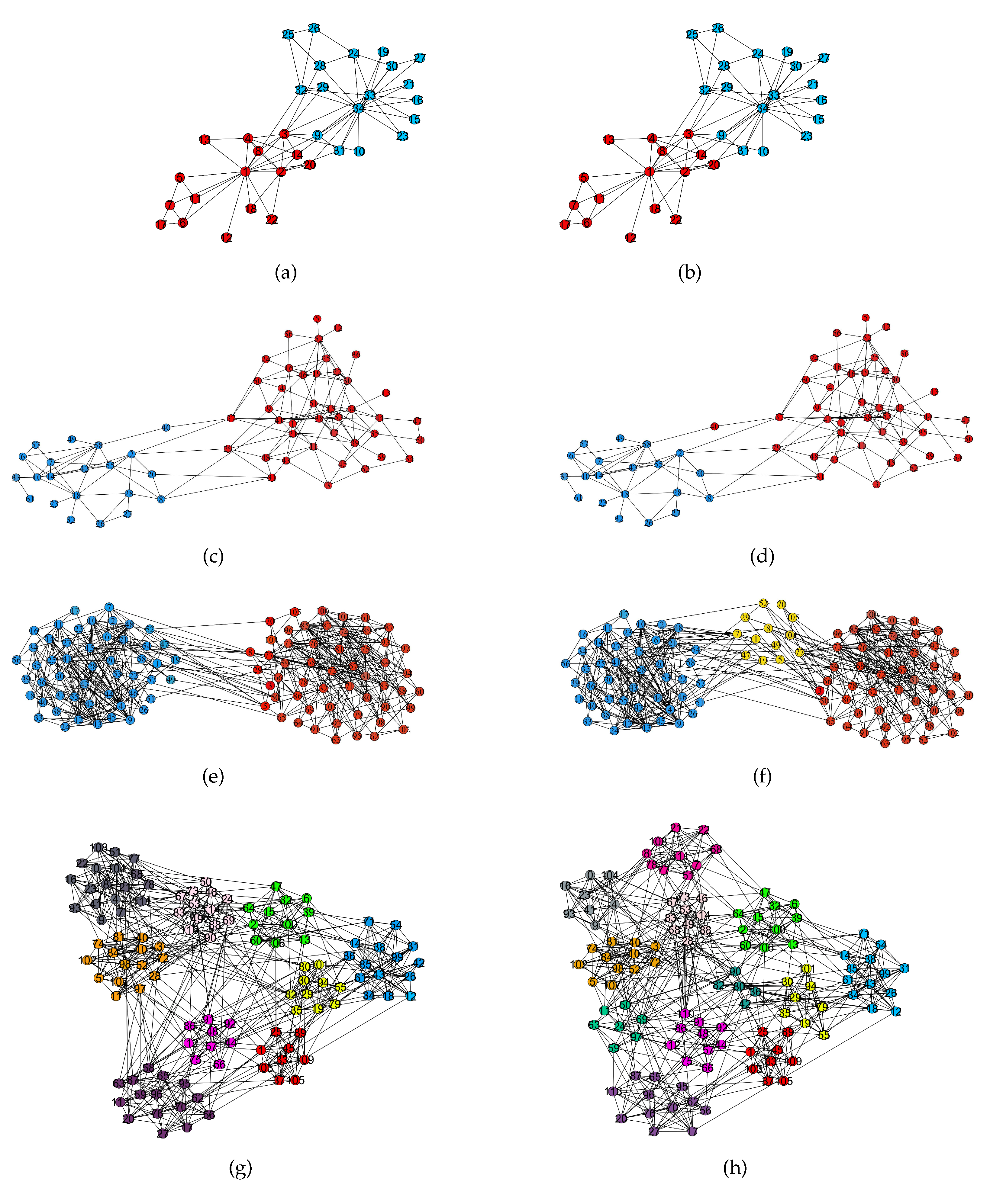
are used to measure the quality of the communities, which are detected by RWBS on the network with ground-truth. The number of seed nodes affects the detected community structure for different networks. The results of the comparison between the communities detected by RWBS and the real communities of the network are shown in
Figure 9.
For the Karate network, it contains two communities, so let the number of seed nodes be 2. In this case,
and
. As can be seen from
Figure 9, the community detected by RWBS at this case is consistent with its real community structure. For the Dolphin network, when the number of seed nodes is 2,
and
. RWBS only divides node 40 to the wrong community and divides the other nodes to the correct community. This is almost consistent with the real community structure of the Dolphin network. For the Political network, it contains three communities, so let the number of seed nodes be 3. In this case,
and
. The real community structure of the network is shown in
Figure 9(f), which contains three communities. Although the proposed algorithm detects the number of communities of this network is two, the quality of the obtained communities is satisfactory. For the Football network, the number of seed nodes is 12,
and
. RWBS detected that it contains 9 communities, and the division result is consistent with its real community structure. In summary, RWBS can find satisfactory communities when the number of seed nodes is
c for networks with ground-truth.
To further show the superiority of RWBS in detecting communities, we selected Walktrap [
10], LPA [
12], KL [
13], SLPA [
31], CDME [
34], and RIIM [
17] as benchmark algorithms.
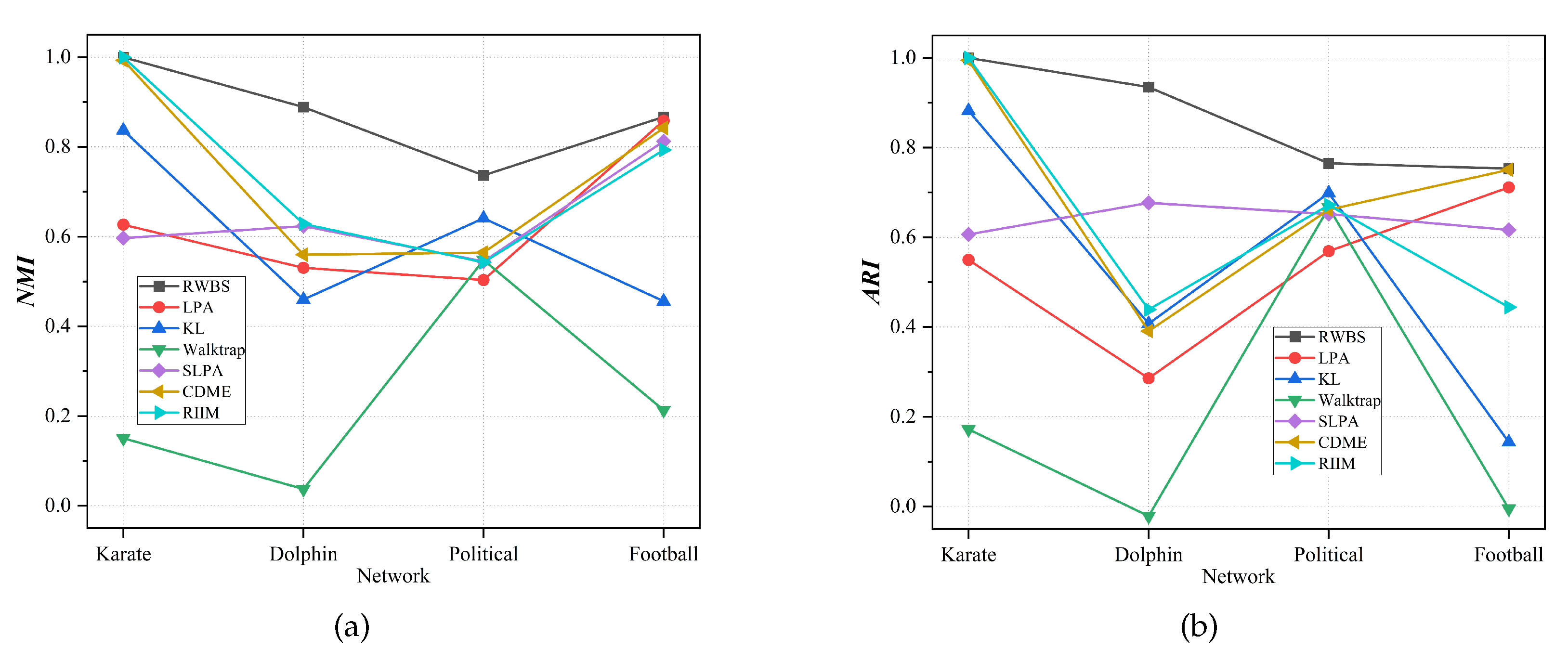
Table 4 and
Figure 10 show the results of the comparison between RWBS and benchmark algorithms in terms of
and
. From
Table 4 and
Figure 10, it can be seen that the results on the networks with ground-truth obtained by RWBS have maximum values in terms of
and
. Moreover, the division result obtained by RIIM on the Karate network is consistent with its real community structure. CDME (LPA and CDME) can also achieve satisfactory results on the Karate (Football) network. Walktrap detects poor community structures on these four networks.
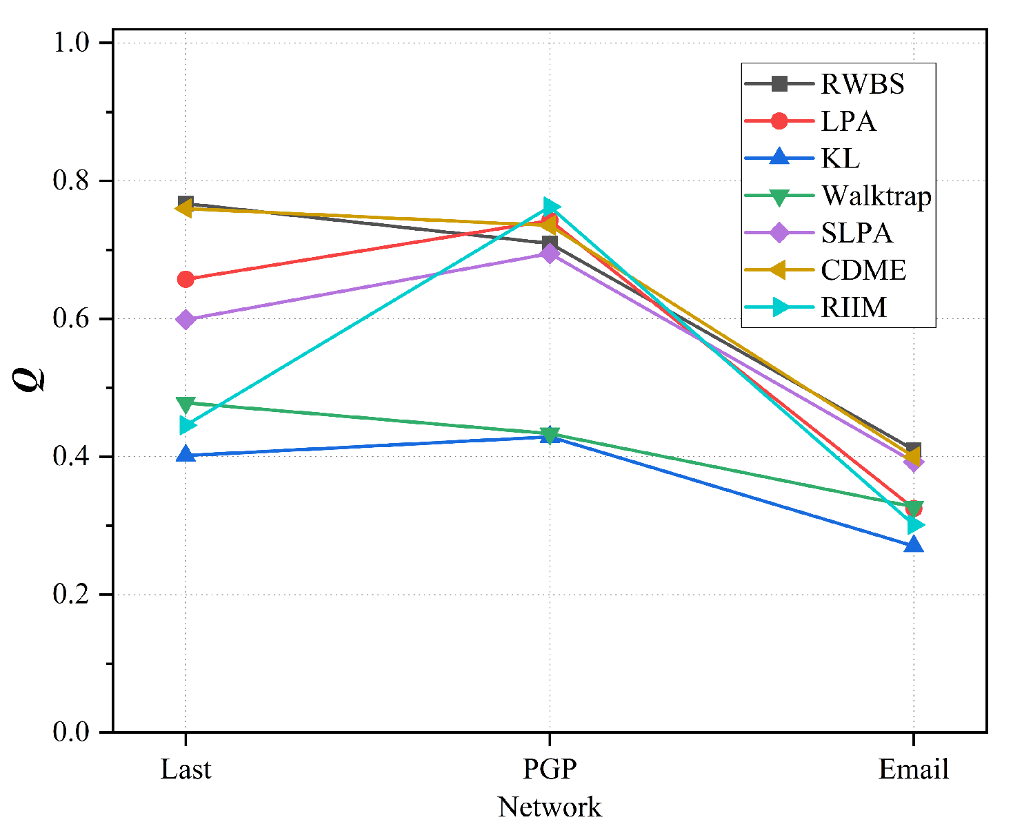
We use
Q as the metric to measure the quality of detected communities on networks without ground-truth. We let the number of seed nodes be
. Comparison results between RWBS and benchmark algorithms in terms of
Q are shown in
Table 5 and
Figure 11. RWBS can obtain the maximum
Q values on Last and Email networks, CDME can also achieve satisfactory
Q values on both networks. For PGP network, RIIM can obtain the maximum
Q value. RWBS, LAP, and CDME can also obtain large
Q (they all have
Q values more than 0.7).
5.2. Experiment on Synthetic Networks
We synthesize networks with the community structure by the LFR model [
54]. Next, we further test the effectiveness of RWBS on these synthesized benchmark networks. Parameters of this model are shown in
Table 6.
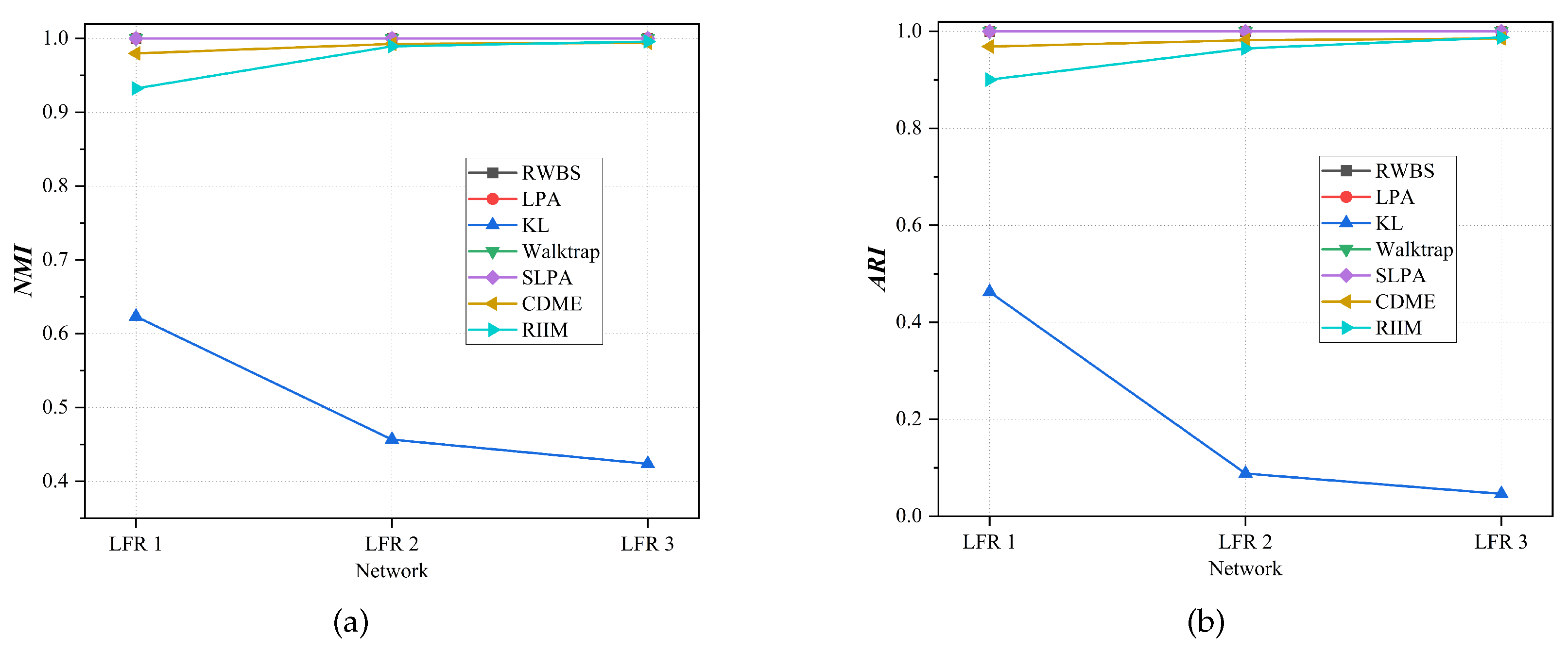
We use RWBS and the benchmark algorithm to detect the community, and use
and
to measure the quality of the detected communities. The comparison results are shown in
Table 7 and
Figure 12. The community structures detected by RWBS, LPA, Walktrap, and SLPA on these three networks are completely consistent with their real community structures. The community structures detected by CDME and RIIM do not completely consistent with their real community structures, but satisfactory results can still be obtained. KL detected poor communities on these three networks.
6. Results and Discussion
In this study, we propose a new random walk algorithm based on different seed nodes for community detection, named RWBS. The mixed centrality is proposed to measure the importance of nodes. According to the value of , the similarity between nodes is calculated. Let the number of seed nodes of networks with (without) ground-truth is c (). For networks with and without ground-truth, based on , we propose algorithms to obtain seed nodes of the random walk, respectively. Furthermore, RWBS changes the transition probability matrix of the random walk algorithm and sets the number of steps of random walk to 6 according to the six degrees separation theory. We use a new label propagation rule that lets labels be updated in a fixed direction. Finally, modularity (Q) is chosen as an optimization function to combine communities, which can optimize the structure of communities. Experimental results on the network also verify the superiority of the RWBS algorithm.
We hope to generalize the RWBS algorithm to other networks in the future, such as directed networks, signature networks, weighted networks, etc. Moreover, we also hope to discover other strategies to find random walk seed nodes for better community division results.
Author Contributions
Writing—original draft, W.L.; validation, J.C. and X.Z.; writing—review and editing, J.C.; methodology, J.C. and J.W. All authors have read and agreed to the published version of the manuscript.
Funding
This research was funded by NSFC grant numbers 12071351, 11971311 and 12161141003 and STCSM grant number 22JC1403602.
Data Availability Statement
Conflicts of Interest
The authors declare no conflicts of interest.
References
- Watts, D.-J.; Strogatz, S.-H. Collective dynamics of small world networks. Nature 1998, 393, 440–442. [Google Scholar] [CrossRef]
- Barabási, A.-L.; Albert, R. Emergence of scaling in random networks. Science 1999, 286, 509–512. [Google Scholar] [CrossRef]
- Barabási, A.-L. Scale-free networks: a decade and beyond. Science 2009, 325, 412–413. [Google Scholar] [CrossRef]
- Newman, M.E.J. The structure of scientific collaboration networks. Proc. Natl. Acad. Sci. 2001, 98, 404–409. [Google Scholar] [CrossRef]
- Girvan, M.; Newman, M.E.J. Community structure in social and biological networks. Proc. Natl. Acad. Sci. 2002, 99, 7821–7826. [Google Scholar] [CrossRef] [PubMed]
- Scott, J. Social Network Analysis, 4th Edition.; SAGE Publications: London, UK, 2017. [Google Scholar]
- Arularasan, A.N.; Suresh, A.; Seerangan, K. Identification and classification of best spreader in the domain of interest over the social networks. Cluster Comput. 2018, 3, 1–11. [Google Scholar] [CrossRef]
- Redner, S. How popular is your paper? an empirical study of the citation distribution. The European Physical Journal B 1998, 4, 131–134. [Google Scholar] [CrossRef]
- Guimerà, R.; Nunes Amaral, L. Functional cartography of complex metabolic networks. Nature 2005, 433, 895–900. [Google Scholar] [CrossRef] [PubMed]
- Pons, P.; Latapy, M. Computing Communities in Large Networks Using Random Walks. Computer and Information Sciences 2005, 3733, 284–293. [Google Scholar]
- Jiao, Q.J.; Huang, Y.; Shen, H.B. Community mining with new node similarity by incorporating both global and local topological knowledge in a constrained random walk. Physica A: Statistical Mechanics and its Applications 2015, 424, 363–371. [Google Scholar]
- Raghavan, U.N.; Albert, R.; Kumara, S. Near linear time algorithm to detect community structures in large-scale networks. Phys. Rev. E 2007, 76, 036106. [Google Scholar] [CrossRef]
- Kernighan, B.W.; Lin, S. An efficient heuristic procedure for partitioning graphs. The Bell System Technical Journal 1970, 49, 291–307. [Google Scholar] [CrossRef]
- Barnes, E.R. An Algorithm for Partitioning the Nodes of a Graph. SIAM Journal on Algebraic Discrete Methods 1982, 3, 541–550. [Google Scholar] [CrossRef]
- Fortunato, S. Community Detection in Graphs. Physics Reports 2010, 486, 75–174. [Google Scholar] [CrossRef]
- Dhumal, A.; Kamde, P.M. Survey on Community Detection in Online Social Networks. International Journal of Computer Applications 2015, 121, 35–41. [Google Scholar] [CrossRef]
- Ullah, A.; Wang, B.; Sheng, J.; Long, J.; Khan, N.; Ejaz, M. A novel relevance-based information interaction model for community detection in complex networks. Expert Systems With Applications 2022, 196, 116607. [Google Scholar] [CrossRef]
- Liu, X.; Murata, T. An Efficient Algorithm for Optimizing Bipartite Modularity in Bipartite Networks. Journal of Advanced Computational Intelligence and Intelligent Informatics 2010, 14, 408–415. [Google Scholar] [CrossRef]
- Newman, M.E.J. Modularity and community structure in networks. Proc. Natl. Acad. Sci. 2006, 103, 8577–8522. [Google Scholar] [CrossRef] [PubMed]
- Newman, M.E.J. Fast algorithm for detecting community structure in networks. Phys. Rev. E 2004, 69, 066133. [Google Scholar] [CrossRef]
- Blondel, V.D.; Guillaume, J.; Lambiotte, R.; Lefebvre, E. Fast Unfolding of Communities in Large Networks, J. Stat. Mech. 2008, P10008. [Google Scholar] [CrossRef]
- Guimerà, R.; Amaral, L.A.N. Functional cartography of complex metabolic networks. Nature 2005, 433, 895–900. [Google Scholar] [CrossRef]
- Boettcher, S.; Percus, A.G. Optimization with Extremal Dynamics. Phys. Rev. Lett 2001, 86, 5211. [Google Scholar] [CrossRef] [PubMed]
- Duch, J.; Arenas, A. Community detection in complex networks using extremal optimization. Phys. Rev. E 2005, 72, 027104. [Google Scholar] [CrossRef] [PubMed]
- M’Barek, M.B.; Borgi, A.; Bedhiafi, W.; Hmida, S.B. Genetic Algorithm for Community Detection in Biological Networks. Procedia Computer Science 2018, 126, 195–204. [Google Scholar] [CrossRef]
- Chen, K.; Bi, W. A new genetic algorithm for community detection using matrix representation method. Physica A: Statistical Mechanics and its Applications 2019, 535, 122259. [Google Scholar] [CrossRef]
- Pourabbasi, E.; Majidnezhad, V.; Afshord, S.T.; Jafari, Y. A new single-chromosome evolutionary algorithm for community detection in complex networks by combining content and structural information. Expert Systems with Applications 2021, 186, 115854. [Google Scholar] [CrossRef]
- Su, Y.; Zhou, K.; Zhang, X.; Cheng, R.; Zheng, H. A parallel multi-objective evolutionary algorithm for community detection in large-scale complex networks. Information Sciences 2021, 576, 374–392. [Google Scholar] [CrossRef]
- Page, L.; Brin, S.; Motwani, R.; Winograd, T. The Pagerank Citation Ranking: Bring Order To The Web. Technical Report, Stanford University, 1998.
- Rosvall, M.; Bergstrom, C.T. Maps of random walks on complex networks reveal community structure. Proc. Natl. Acad. Sci. 2008, 105, 1118–1123. [Google Scholar] [CrossRef]
- Xie, J.; Szymanski, B.K.; Liu, X. SLPA: Uncovering Overlapping Communities in Social Networks via a Speaker-Listener Interaction Dynamic Process. In 2011 IEEE 11th International Conference on Data Mining Workshops, Vancouver, BC, Canada, IEEE, 2011, 344–349.
- Laassem, B.; Idarrou, A.; Boujlaleb, L.; Iggane, M. Label propagation algorithm for community detection based on Coulomb’s law. Physica A: Statistical Mechanics and its Applications 2022, 593, 126881. [Google Scholar] [CrossRef]
- Fang, W.; Wang, X.; Liu, L; Wu, Z.; Tang, S.; Zheng, Z. Community detection through vector-label propagation algorithms. Chaos, Solitons & Fractals 2022, 158, 112066. [Google Scholar]
- Sun, Z.; Sun, Y.; Chang, X.; Wang, Q.; Yan, X.; Pan, Z.; Li, Z. Community detection based on the Matthew effect. Knowledge-Based Systems 2020, 205, 106256. [Google Scholar] [CrossRef]
- Chen, X.; Hu, J.; Chen, Y. GBTM: Community detection and network reconstruction for noisy and time-evolving data. Information Sciences 2024, 679, 121069. [Google Scholar] [CrossRef]
- Danon, L.; Duch, J.; Diaz-Guilera, A.; Arenas, A. Comparing community structure identification. Journal of Statistical Mechanics: Theory and Experiment, 0900. [Google Scholar]
- Rand, W.M. Objective criteria for the evaluation of clustering methods. Journal of the American Statistical Association 1971, 66, 846–850. [Google Scholar] [CrossRef]
- Kim, Y.; Son, S.-W.; Jeong, H. Finding communities in directed networks. Phys. Rev. E 2010, 81, 016103. [Google Scholar] [CrossRef] [PubMed]
- Bonacich, P.F. Factoring and weighting approaches to status scores and clique identification, J. Math. Sociol. 1972, 2, 113–120. [Google Scholar] [CrossRef]
- Newman, M.E.J. A measure of betweenness centrality based on random walks. Social Networks 2005, 27, 39–54. [Google Scholar] [CrossRef]
- Freeman, L.C. Centrality in social networks conceptual clarification. Social Networks 1978, 1, 215–239. [Google Scholar] [CrossRef]
- Stephenson, K.; Zelen, M. Rethinking centrality: Methods and examples. Social Networks 1989, 11, 1–37. [Google Scholar] [CrossRef]
- Brin, S.; Page, L. The anatomy of a large-scale hypertextual web search engine. Comput. Netw. ISDN Syst. 1998, 30, 107–117. [Google Scholar] [CrossRef]
- Wasserman, S.; Faust, K. Social Network Analysis: Methods and Applications, first ed.: Cambridge University, New York, 1994.
- Ren, Z.; Shao, F.; Liu, J.; Guo, Q.; Wang, B. Node importance measurement based on the degree and clustering coefficient information. Acta Phys. Sinica 2013, 62, 128901. [Google Scholar]
- Tong, H.; Faloutsos, C.; Pan, J.Y. Fast random walk with restart and its applications, In Sixth International Conference on Data Mining, Hong Kong, China, IEEE, 2006, 613–622.
- Hua, J.; Yu, J.; Yang, M.S. Fast clustering for signed graphs based on random walk gap. Social Networks 2020, 60, 113–128. [Google Scholar] [CrossRef]
- Zachary, W.W. An information flow model for conflict and fission in small groups. Journal of Anthropological Research 1997, 33, 452–473. [Google Scholar] [CrossRef]
- Lusseau, D.; Schneider, K.; Boisseau, O.; Haase, P.A.; Slooten, E.; Dawson, S. The bottlenose dolphin community of doubtful sound features a large proportion of long-lasting associations. Behavioral Ecology and Sociobiology 2003, 54, 396–405. [Google Scholar] [CrossRef]
- Newman, M.E.J.; Girvan, M. Finding and evaluating community structure in networks. Phys. Rev. E 2004, 69, 026113. [Google Scholar] [CrossRef] [PubMed]
- Toivonen, R.; Kovanen, L.; Kivelä, M.; Onnela, J.; Saramäki, J.; Kaski, K. A comparative study of social network models: Network evolution models and nodal attribute models. Social Networks 2009, 31, 240–254. [Google Scholar] [CrossRef]
- Boguñá, M.; Pastor-Satorras, R.; Díaz-Guilera, A.; Arenas, A. Models of social networks based on social distance attachment. Phys. Rev. E 2004, 70, 056122. [Google Scholar] [CrossRef] [PubMed]
- Rossi, R.A.; Ahmed, N.K. The Network Data Repository with Interactive Graph Analytics and Visualization. In Twenty-Ninth AAAI Conference on Artificial Intelligence, Austin Texas, AAAI Press, 2015, 4292–4293.
- Lancichinetti, A.; Fortunato, S.; Radicchi, F. Benchmark graphs for testing community detection algorithms. Phys. Rev. E 2008, 78, 046110. [Google Scholar] [CrossRef]
Figure 1.
The network with 27 nodes and 26 edges.
Figure 1.
The network with 27 nodes and 26 edges.
Figure 2.
The correlation between the decline rate of network efficiency and the importance of nodes ranked by , , and . (a) . (b) . (c) .
Figure 2.
The correlation between the decline rate of network efficiency and the importance of nodes ranked by , , and . (a) . (b) . (c) .
Figure 3.
A network to explain the transfer probability of node i.
Figure 3.
A network to explain the transfer probability of node i.
Figure 4.
The structure of the triangle.
Figure 4.
The structure of the triangle.
Figure 5.
(a) The sample network with 9 nodes and 15 edges. (b) The real community structure of the sample network.
Figure 5.
(a) The sample network with 9 nodes and 15 edges. (b) The real community structure of the sample network.
Figure 6.
The value of .
Figure 6.
The value of .
Figure 7.
The value of w when .
Figure 7.
The value of w when .
Figure 8.
The label propagation process when .
Figure 8.
The label propagation process when .
Figure 9.
Comparison results obtained by RWBS with the real division result on real-world networks with ground-truth. (a) The division result obtained by RWBS (, , ). (b) The real community structure of the Karate network (). (c) The division result obtained by RWBS (=0.8889, , ). (d) The real community structure of the Dolphin network (). (e) The division result obtained by RWBS (=0.7365, , ). (f) The real community structure of the Political network (). (g) The division result obtained by RWBS (=0.8671, , ). (h) The real community structure of the Football network ().
Figure 10.
Comparison results between RWBS and benchmark algorithms on networks with ground-truth in terms of and (The values of LPA, SLPA, and CDME are averages obtained by running 10 experiments independently). (a) NMI. (b) ARI.
Figure 10.
Comparison results between RWBS and benchmark algorithms on networks with ground-truth in terms of and (The values of LPA, SLPA, and CDME are averages obtained by running 10 experiments independently). (a) NMI. (b) ARI.
Figure 11.
Comparison results on networks without ground-truth in terms of Q (The values of LPA, SLPA, and CDME are averages obtained by running 10 experiments independently).
Figure 11.
Comparison results on networks without ground-truth in terms of Q (The values of LPA, SLPA, and CDME are averages obtained by running 10 experiments independently).
Figure 12.
Comparison results between RWBS and benchmark algorithms on synthetic networks in terms of and (The values of LPA, SLPA, and CDME are averages obtained by running 10 experiments independently). (a) NMI. (b) ARI.
Figure 12.
Comparison results between RWBS and benchmark algorithms on synthetic networks in terms of and (The values of LPA, SLPA, and CDME are averages obtained by running 10 experiments independently). (a) NMI. (b) ARI.
Table 1.
The definitions of other mathematical symbols used in this paper.
Table 1.
The definitions of other mathematical symbols used in this paper.
| Symbol |
Definition |
| n |
The number of nodes |
| m |
The number of edges |
|
The degree of node i
|
|
The label of node i
|
|
The community to which node i belongs |
| c |
The number of communities. |
|
The neighbor nodes of node i
|
|
The restart probability |
|
The set of labels that have been updated times |
|
The maximum degree of the nodes on the network |
|
The average degree of the network |
Table 2.
The information of nodes
Table 2.
The information of nodes
| Information |
1 |
2 |
3 |
4 |
5 |
6 |
7 |
8 |
9 |
|
3 |
4 |
4 |
3 |
3 |
4 |
3 |
3 |
3 |
|
0.3750 |
0.5000 |
0.5000 |
0.3750 |
0.3750 |
0.5000 |
0.3750 |
0.3750 |
0.3750 |
|
0.0625 |
0.0667 |
0.0833 |
0.0625 |
0.0500 |
0.0769 |
0.0556 |
0.0556 |
0.0556 |
|
0.8643 |
0.9835 |
1.0000 |
0.8643 |
0.8536 |
0.9936 |
0.8583 |
0.8583 |
0.8583 |
Table 3.
The information of real networks
Table 3.
The information of real networks
| Network |
n |
m |
|
|
c |
| Karate |
34 |
78 |
17 |
4.588 |
2 |
| Dolphin |
62 |
159 |
12 |
5.129 |
2 |
| Political |
105 |
441 |
25 |
8.400 |
3 |
| Football |
115 |
616 |
12 |
10.661 |
12 |
| Last |
8003 |
16824 |
46 |
4.204 |
- |
| PGP |
10K
|
24K
|
206 |
4.558 |
- |
| Email |
33K
|
180K
|
1383 |
10.732 |
- |
Table 4.
Comparison results on real networks with ground-truth (The values of LPA, SLPA, and CDME are averages obtained by running 10 experiments independently).
Table 4.
Comparison results on real networks with ground-truth (The values of LPA, SLPA, and CDME are averages obtained by running 10 experiments independently).
| Approaches |
Karate |
Dolphin |
| |
|
|
|
|
| RWBS |
1 |
1 |
0.8889 |
0.9348 |
| LPA |
|
|
|
|
| KL |
0.8372 |
0.8823 |
0.4599 |
0.4077 |
| Walktrap |
0.1507 |
0.1722 |
0.0374 |
-0.0213 |
| SLPA |
|
|
|
|
| CDME |
|
|
|
|
| RIIM |
|
|
|
|
| Approaches |
Political |
Football |
| |
|
ARI |
|
|
| RWBS |
0.7365 |
0.7648 |
0.8671 |
0.7530 |
| LPA |
|
|
|
|
| KL |
0.6409 |
0.6987 |
0.4560 |
0.1437 |
| Walktrap |
0.5478 |
0.6661 |
0.2132 |
-0.0050 |
| SLPA |
|
|
|
|
| CDME |
|
|
0.84220.0364 |
0.75060.1306 |
| RIIM |
|
|
|
|
Table 5.
Comparison results on real networks without ground-truth (The values of LPA, SLPA, and CDME are averages obtained by running 10 experiments independently).
Table 5.
Comparison results on real networks without ground-truth (The values of LPA, SLPA, and CDME are averages obtained by running 10 experiments independently).
| Approaches |
Last |
PGP |
Email |
| |
|
|
|
|
|
|
| RWBS |
183 |
0.7671 |
197 |
0.7094 |
62 |
0.4102 |
| LPA |
|
|
|
|
|
|
| KL |
2 |
0.4017 |
2 |
0.4290 |
2 |
0.2703 |
| Walktrap |
1358 |
0.4783 |
1753 |
0.4335 |
353 |
0.3273 |
| SLPA |
|
|
|
|
|
|
| CDME |
|
|
|
|
|
|
| RIIM |
606 |
0.4457 |
560 |
|
521 |
|
Table 6.
Parameters of LFR
Table 6.
Parameters of LFR
| Networks |
n |
|
|
|
|
|
| LFR 1 |
100 |
20 |
10 |
20 |
30 |
0.1 |
| LFR 2 |
1000 |
50 |
30 |
40 |
50 |
0.1 |
| LFR 3 |
2000 |
50 |
30 |
45 |
50 |
0.1 |
Table 7.
Comparison results on synthetic networks (The values of LPA, SLPA, and CDME are averages obtained by running 10 experiments independently).
Table 7.
Comparison results on synthetic networks (The values of LPA, SLPA, and CDME are averages obtained by running 10 experiments independently).
| Approaches |
LFR 1 |
LFR 2 |
LFR 3 |
| |
|
|
|
|
|
|
| RWBS |
1 |
1 |
1 |
1 |
1 |
1 |
| LPA |
|
|
1 |
1 |
1 |
1 |
| KL |
0.6233 |
0.4627 |
0.4565 |
0.0881 |
0.4237 |
0.0462 |
| Walktrap |
1 |
1 |
1 |
1 |
1 |
1 |
| SLPA |
|
|
|
|
1 |
1 |
| CDME |
|
|
|
|
|
|
| RIIM |
|
|
|
|
|
|
|
Disclaimer/Publisher’s Note: The statements, opinions and data contained in all publications are solely those of the individual author(s) and contributor(s) and not of MDPI and/or the editor(s). MDPI and/or the editor(s) disclaim responsibility for any injury to people or property resulting from any ideas, methods, instructions or products referred to in the content. |
© 2024 by the authors. Licensee MDPI, Basel, Switzerland. This article is an open access article distributed under the terms and conditions of the Creative Commons Attribution (CC BY) license (http://creativecommons.org/licenses/by/4.0/).
