
Submitted:
05 July 2024
Posted:
08 July 2024
You are already at the latest version
Abstract
The daily path of the Sun across longitude yields night and day, but the Sun also travels across latitude on a belt 47° wide. The Sun meridian declination explains the annual budget of natural beam irradiance (NBI), which is the irradiance delivered to the Earth’s surface as a normal projec-tion from the Sun. Data for the sun meridian declination data were obtained from the geometric model. The distribution of NBI was weighed between the Tropics of Cancer and Capricorn. The variation patterns of the solar declination conform to the dynamics of pendular motion. The joint distributions of velocity or acceleration of meridian declination against declination fit circular graphs. The NBI budget fluctuates in inverse proportion to the velocity of declination, yielding 18 sun-paths per degree for latitudes above 20°, and 6 sun-paths per degree for latitudes under 20°. All sites of the planet, whose latitude coincide, whether within or between hemispheres, accumu-late an equivalent budget of NBI.
Keywords:
solar-heat distribution
; solar-light distribution
; Sun-Earth Physics
; normal irradiance
; climate
; lumbra
; exposure term to NBI
; resting term from NBI
1. Introduction
Solar radiation works as the unifying force that shapes all physical and biological elements of the planet [1,2]. The climate system is initiated by solar heat [3] while solar light fuels photosynthesis [2,3]. The annual cycle of solar declination is the primary factor driving the distribution of the Earth’s climatic zones [3]. Small variations in solar irradiance scale climate responses globally [4]. For instance, surface temperatures rise 0.1°C when solar irradiance increases 0.1% [5]. The temperature of a site increases as the solar declination approaches the site’s latitude, and decreases as the solar declination departs from that latitude [6].
In Sciences of Energy, the global irradiance has been usually split in direct normal irradiance (DNI) and diffuse irradiance. DNI is defined as the radiation coming from the solar disk, received by a plate placed normal to the Sun [7] measured within a solid angle of up to 20° centered in the solar disk [7]. Because DNI can be assessed whenever a plate points the Sun and wherever the Sun is visible, such concept proves ineffective in explaining the latitudinal distribution of the Earth’s budget of solar radiation; hence, the present work introduces several definitions aimed to analyzing the irradiance supplied to the planet at the local meridian. Natural beam irradiance (NBI) denotes the share of the global irradiance that occurs as a normal projection to the Earth’s surface when the solar disk (only 32 arcmin wide) occupies the local zenith. NBI is exclusive to the subsolar point and can only occur between the Tropics of Cancer and Capricorn, while it does not consider solid angles beyond the angular size of the Sun. Natural oblique irradiance (NOI) denotes the share of the global irradiance that is supplied to a given site when the solar disk crosses the local meridian, so that NOI always lands at angles below 90°, while it can only occur at solar noon. NOI conforms a line that pairs with a meridian (where the center of such line holds NBI) and spans the Earth across all longitudes within a day (24 h), following the planet’s rotation. The angle at which NOI lands, depends on the angular distance between the belt holding NBI and the belt in which NOI is recorded. The obliquity angle of NOI remains unchanged for a given latitude along the day.
The angle at which the sunrays strike a site at the local meridian (NOI obliquity) fluctuates on a daily basis, as a consequence of the annual cycle of solar declination. Every day, the Sun declination switches latitude, traveling the planet to a variable velocity. Conversely, the sunrays’ absolute perpendicularity, and its inherent NBI, occur to a particular latitude only twice within a Gregorian year; when the solar declination converges that latitude on its way south, and then northwards. Nonetheless, it can involve several instances within a season when the velocity of solar meridian declination promotes Sun-path overlapping. But even on the days of sunrays perpendicularity, NBI occurs to a given longitude for merely 2.2 minutes, which is the time it takes for the apparent Sun to cross the local meridian from east to west: 15 arcdeg hour-1, or 2.2 minutes for the 32 arcmin (angular size of the Sun).
If the Sun, whose diameter is 109 times larger than that of the Earth, could cast an umbra of light on the subsolar point, the diameter of such light umbra might be comparable to the lunar umbra that appears during an annular eclipse. The given comparison is valid because of the equivalence in the angular sizes of the Sun and the Moon [8], as perceived from Earth. Despite the Sun’s diameter being 400 times larger than that of the Moon, it is located 388 times farther from Earth than the satellite. Moreover, when the circumference of the planet is divided by 360°, it yields 111.3 km arcdeg-1, which derives in a diameter of 60 km for the lumbra, given than the solar disk only covers 32 arcmin. The great disparity in diameters between the solar disk (1.392x10⁶ km) and the lumbra (let it be 60 km) yields a ratio of 23000:1. Accordingly, the sunrays’ bundle that is normally projected from the Sun to the Earth takes the shape of a cone of light, which extends from the solar disk to the lumbra, and its axis vector extends from the center of the solar disk to the subsolar point.
That NBI is significantly higher at the subsolar point, is supported by several facts. (1) If light travels on a straight path [9] and a straight line is the shortest distance between two points (known facts), then the subsolar point is the closest spot to the Sun on the entire Earth [10]. (2) The sunrays that are delivered perpendicularly to the Earth, cross the atmosphere through its shortest dimension [11]; whereas those obliquely delivered interact with the atmosphere for tens of kilometers [12]; and (3) the Sun and the lumbra differ widely in diameters.
The Sun meridian declination defines the only latitude of the planet that receives the light cone, the lumbra, and therefore NBI, within a period of 24 hours, despite the Sun illuminating and heating half the globe at a time. When the apparent Sun reaches the zenith in the visible sky, the sunrays strike the land and the ocean at a right angle (90°), accounting for the highest power density received by a site throughout the year. As the power density of the sunrays decreases on par with their obliquity [13]; the subsolar point [10] holds the highest NBI budget compared to any other site on the entire planet.
The Sun radius is 696,340 km; hence, the sunrays coming from its edge are emitted at an increased distance of 696,340 km as compared to those of coming from the Sun center (1.8 times the Earth-Moon distance). The sunrays from the center shall supply a higher concentration of heat and light to the Earth than those from the edge. The brightness of the solar disk declines from the core to the limb, while its temperature drastically drops beyond the chromosphere [14]. Every solar path whose angle of declination approaches a given latitude, comprises a significant share to the total irradiance a site accumulates throughout the year [7].
Because the sunrays can only reach normality at noon, NBI must be assessed by means of the solar meridional declination. Assuming that the radiation intended for the Earth remains constant between two consecutive days (at a distance Sun-Earth of 1 UA, the budget of NBI can be assessed from the velocity of the Sun declination for the inter-tropics. The present work aims to assess the budget of NBI for latitudes between the Tropics of Cancer and Capricorn, which is in close association with the budget of solar resources (heat and light) that every latitude can harness throughout the year. The working hypotheses are: (1) the velocity and acceleration of the Sun meridian declination vary on par with latitude; (2) the velocity of solar meridian declination allows for an easy assessment of the annual budget of NBI for every latitude where it occurs; & (3) a similar budget of NBI characterize every range of latitude.
2. Materials and Methods
2.1. Data
Data for the Sun meridian declination () was generated from the geometric model [15] (Equation (2)), which is valid for any Gregorian year. The Spencer model takes ground on the fractional year, in radians (Equation (1)), which considers the time as the number of days within the year, from 1 to 365.
The velocity () and acceleration () of solar meridian declination (), were assessed as the first- (Equation (3)) and second order (Equation (4)) derivatives of the position (). The parameters , and arise in arcdeg, arcdeg day-1 or arcdeg day-2, respectively, by applying the factor to Equations (2) to (4) ( and ); given that the Spencer model yields data in radians. Derivatives were obtained applying the chain rule; for instance, the derivative is assessed by the product (). The Equation of Time (E) was assessed for a one-year period, following the geometric model of Spencer [15] (Equation (5)). E also includes a factor of (4), which converts units from arcdeg to time (minutes). The variable indicates the time in days, from 1 to 365 and is the fractional year in radians.
2.2. Variables
The Sun meridian declination () was assessed for every day of two non-leap Gregorian years, to represent its cyclical nature. The angular velocity () and angular acceleration () of the solar meridian declination ( were assessed for the same period. The geometric model yields a unique record of solar declination for every day within a Gregorian year; hence, the chosen unit for time unit was day.
2.3. Defining New Variables and Suitable Units
When assessing and as the first- and second order derivatives of , the records of each derivative in turn, fell in a range of 1/60th of the range in which the records of its integral occurred. The values of , and take place in the ranges -23.5 to 23.5 arcdeg, -0.3896 to 0.3953 arcdeg day-1 and -0.0069 to 0.0078 arcdeg day-2, respectively. From such parameters, the variables and are derived; where , while = 3600. The units of and can be switched to arcmin day-1 and arcsec day-2, respectively. After unit transformation, the variables , and fall within the range 0 to 28.5.
Renaming parameters and switching units served several purposes: (1) to avoid too small records lacking an integer component, (2) to represent the three parameters on a unified ordinate axis despite their differing dimensions; and (3) to illustrate the resemblance and associations between the functions of , and when plotted, first against time (days within a year) and then against E.
2.4. Declination Cycle
The meridian declination (), angular velocity () and acceleration () of the apparent Sun, were plotted against the Equation of Time (E); where E is defined as the difference between the mean time and the solar time, and comprises the abscise of the meridional analemma. The signs were kept positive when was above the Equator, when corresponded to a shift of declination to the north (winter or spring), when corresponded to a southern declination, or when the E occurred to the right of the meridian. Conversely, all signs were kept negative when was below the Equator, when corresponded to a shift of declination to the south (summer and autumn), when corresponded to a northern declination, or when the E occurred to the left of the meridian.
All signs were disregarded and data from both hemispheres combined, because that the signs indicate the direction of the resultant drive rather than magnitude. The meridian declination, velocity and acceleration of the Sun were plotted on the E, obtaining three analemma-like shapes in the same chart.
2.5. Arbitrary Belts
Five latitudinal belts were arbitrarily proposed on each hemisphere, from the Equator to either the Tropic of Cancer or Capricorn. Four belts (denoted Equatorial, A, B, C) framed 5 arcdeg each, while the fifth (denoted Tropical) framed only 3.5 arcdeg. The last belt was intentionally thinner to emphasize the fact that the NBI is expected to last longer on this belt.
Data were assessed within hemisphere. Later, all belts with equivalent limits of latitude were averaged together, disregarding the current direction of the cycle of solar declination or the hemisphere to which they belonged, because every belt has a corresponding belt in the opposite hemisphere, regarding the latitudinal range. For instance, two sections of the declination cycle span the arbitrary belt denoted A (5,10] during spring (5,10] and summer [10,5), while two sections span a corresponding range of latitude on the opposing hemisphere during autumn (-5, -10] and winter [-10, -5).
2.6. Exposure and Resting Terms, and Budget of NBI
As the Sun declination cycle spans the very same arbitrary belt twice a year, from north to south and then backwards, two additional concepts are proposed. The exposure term denotes the period on which an arbitrary belt holds NBI, whereas the resting term denotes the period on which an arbitrary belt lacks NBI because the solar declination cycle occurs elsewhere. The daily budget of NBI (, Equation (6)) was assessed as the percentage of the Earth’s annual budget.
The Equation (6) implies that every day within a Gregorian year, the planet receives 0.274% of its annual budget of NBI assuming that the daily budget remains constant between successive days at an average Sun-Earth distance of 1 AU. The result accounts for the relative value of a single Sun-path among the 365 paths of the year. The relative budget of NBI harnessed by an arbitrary belt, (% arcdeg-1) was assessed following Equation (7), where the exposure term is the number of days that the sun lasts on a given belt.
As is the vertical distance between two consecutive records of solar declination, signifies the width of the belt on which the daily budget of NBI () is distributed within a day. The accumulated budget of heat and light delivered to a particular arbitrary belt as NBI vary in association with the . The integrated budget of NBI available for every latitude (% arcdeg-1) was assessed for belts of size and an exposure term of a single day, which yields Equation (8). The given equation for incorporates the factor 60 in order to express the results as a budget of NBI per arcdeg of latitude instead of arcmin.
3. Results
3.1. Declination Cycle
The functions of meridian declination (, arcdeg), angular velocity (, arcmin day-1) and acceleration (, arcsec day-2) of the Sun against time (Figure 1), vary within a similar range, as if they represented the very same variable (except for the wider amplitude of ; although occurs to the left of , and occurs to the left of , by a distance equal to the length of an entire season, in both cases. The functions of , “60, and “3600” (which are numerically identical to , and ) yield pseudo-sinusoidal curves that resemble each other in shape, amplitude and frequency (Figure 1).
Equinoxes are tagged on the Equator (solid circle), and solstices on the Tropics of Cancer and Capricorn (open circle).
According to Figure 1, falls within a range of 1/60th of the interval spanned by , and falls within a range of 1/60th of the interval spanned by ; therefore takes place within a range of 1/3600th of the range span covered by . The original parameters , and keep the same scale (arcdeg), so that the terms 60 and 3600 use the adequate factors but conform to the same scale and units. Afterwards, the incorporation of such factors 60 and 3600 (for and ) allows to define suitable variables for the visuals, where 60 becomes and 3600 becomes . For the visuals, the units of are switched to arcmin day-1 and those of to arcsec day-2; whereas, the units of and remain unchanged to build the formulae.
Following the variables as defined in Equation (2) to 4, the functions and () approximate circumference shapes (Equation (9) and 10). Despite the functions and () being defined in arcdeg for Equation (9) and 10, Figure 2 displays the very same information, as and (), where the factors 60 and 3600 of the mentioned equations are now implicit in the variables, although units have been switched to those of the new variables.
According to Figure 1, the highest can only occur at the lowest and vice versa, while the same holds true between and . Because the pseudo-sinusoidal amplitude of diverge from those of and , the charts on Figure 2 are not flawless circumferences; for instance, the diameters show a slight variation. The radius of Equation (9) fluctuates from 23.2 to 24.3, and average to 23.6; while the radius of Equation (10) fluctuates from 23.0 to 28.1 , and average to 24.5 (Figure 2).
where : solar meridian declination (arcdeg); velocity of solar meridian declination (arcdeg day-1); : acceleration of solar meridian declination (arcdeg day-2), and approaches the actual tilting of the Earth’s axis of rotation (arcdeg)
Equinoxes (solid circle) are tagged in the Equator and solstices (open circle) in the Tropics of Cancer and Capricorn.
The correlation between and , as displayed in Figure 2, which can also be referred as the association between and, exhibits an alternated direct/inverse association (r = ±0.91; P<0.001) from one season to another, suggesting a rhomboidal shape instead of the true circular association (Equation (9)). An analogous pseudo-circumference function (Equation (10), Figure 2) explains the relationship between and , which can also be referred as the association between ) and ), exhibits an alternated direct/inverse association (r = ±0.93; P<0.001) as well. Following Figure 1 and 2, the association between , and , or between , ) and becomes clear. The correlation coefficients inform that , , and ; otherwise stated and , whereas .
3.2. Analemmic Charts
The functions of and over E are shown in Figure 3. Most records displayed in quadrants I and II, resemble, mirror and correspond to the values of shown in quadrants III and IV, respectively. Furthermore, most records displayed in quadrant II and IV correspond to spring and summer, while most records shown in quadrants III and I correspond to autumn and winter.
When and were plotted against E (in Figure 3), following the units proposed for the visuals, the three analemmic curves depict lemniscate-shapes whose records fell within a similar range. Since and were previously scaled up through the unit transformation, the real sizes of the and lemniscates are of 1/60th and 1/3600th, respectively, as compared with the analemma () . Unlike and , the sections in quadrants I and II of the lemniscate enclose an area similar to that enclosed by the same curve in the quadrants III and IV; furthermore, such lemniscate becomes slanted to the left.
3.3. Budget of NBI
The solar meridian declination, exposure term, resting term, and the budget of NBI (% arcdeg-1) are shown in Table 1, for each arbitrary belt. In Table 1, the two sections of the Sun declination cycle that provide NBI to each arbitrary belt, are presented separately. The same information presented in Table 1 is shown in Table 2; where the two exposure terms of each particular belt are combined, and data are averaged for both hemispheres.
A lower yields a higher exposure to NBI, therefore the budget of solar heat and light that a site holds increases on par with its latitude from either Equatorial belt to the corresponding Tropical belt (Table 1). The signs of and are always consistent within season, but they do switch between seasons. Hence, the same resultant drive characterizes an entire season, while the next season always presents a contrasting drive. Seasons whose resultant drive is accelerative are characterized by holding the same sign for and , whereas such signs differ for seasons whose resultant drive is decelerative.
In every season, the path of the Sun goes through the five arbitrary belts of a hemisphere; whereas, the average records of , and exhibit a close symmetry both between seasons and between hemispheres. In the northern hemisphere, the arbitrary belts denoted Equatorial, A, B, C and Tropical, hold exposure terms of 24, 29, 30, 37, and 66 Sun-paths (days) throughout the year. This values represent 6.57, 7.94, 8.22, 10.14 and 18.08 % of the Earth’s annual budget of NBI, equivalent to 1.32, 1.59, 1.64, 2.03 and 5.17 % arcdeg-1, respectively.
In the southern hemisphere, the arbitrary belts denoted as Equatorial, A, B, C and Tropical, hold exposure term of 26, 26, 30, 37, and 60 Sun-paths (days) throughout the year. This values represent 7.12, 7.12, 8.22, 10.13 or 16.43 % of the Earth’s annual budget of NBI, equivalent to 1.42, 1.42, 1.64, 2.03 and 4.70 % arcdeg-1, respectively.
The daily budget of NBI (, % arcdeg-1) delivered per arc degree of latitude, assessed as a fraction from annual budget intended for the planet (Eq 4), is shown on Figure 4. The NBI budget of a belt can also be thought of as the quotient between its exposure term (in days) and the number of days in a year. The NBI budget intended for the Tropical belt (20 and 23.5°) is received during a unique exposure term of 66 or 60 days, and followed by a unique resting term 299 or 305 days long, for the northern or southern hemisphere, same order. The belts A, B and C hold two exposure terms of equal length, as well as two resting terms of contrasting length, the shorter the first the longer the second.
In Figure 4, ranges from 0.69 to 4.0 for 327 out of the 365 days, but grows higher during 20 days centered in the summer solstice or 18 days centered in the winter solstice. Illogical records occur near the solstices, which implies that is so slow that many Sun-paths overlap on the very same latitude. The total that each arbitrary belt gathers along the year (Table 2) is the sum of the budgets of the two seasons on which the Sun declination cycle spans the same range of latitude (Table 1). In Figure 4, the budgets of NBI for summer and autumn are displayed as “negative records”, despite they cannot be negative, and they are not; but the chart takes advantage from the sign of to distinguish between summer and spring or between autumn and winter.
4. Discussion
The structure of the information shown in Figure 1, 2, and 3, depends on the units chosen for and . Likewise, approximating the diameter of the circular shapes and , corresponding to Equation (9) and 10 (Figure 2), respectively, can only be possible by scaling up and by the factors specified in the Equations. The similarity in range between the three parameters of solar declination, once scaled up, implies that occurs at a rate of 1/60th, and occurs at a rate of 1/3600th of the range in which befalls.
The variations in , and are typical of oscillatory pendular motion. The annual cycle of solar declination features two equilibrium points at the equinoxes, and two resting points at the solstices. A trough of converges to a peak of at the solstices, where the Sun slows down, comes to a standstill, and then speeds, during the days preceding, the day at, and the days following a solstice, respectively. A trough of converges to a peak of at the Equator, where progressively decreases, reaches zero and then progressively increases, during the days before, the day at, and the days after an equinox, respectively. The apparent Sun progressively brakes during spring or autumn, as it approaches a solstice, while it shows diminishing increments of all through summer or winter.
The association between and fits a circumference, where the spring, summer, autumn and winter lie on the quadrants I, II, III and IV of the circle , respectively. When signs are disregarded, vary in direct proportion to . Every range of latitude conforms to characteristic records of , , and . For example, the four instances of the belt C show comparable records of and , with only slight differences between hemispheres. The dynamics of declination is equivalent between seasons whose resultant drive coincide (spring vs autumn, or summer vs winter), whereas , , and vary in reverse order between for seasons whose resultant drive diverge (spring vs summer, or autumn vs winter).
According to the Sun meridian declination, every arbitrary belt holds NBI during two exposure terms within a year; both of equal length and each followed by a characteristic resting term. The first exposure term occurs when the Sun meridian declination spans an arbitrary belt on its way north, and the second term occurs when the solar declination spans the same belt on its way south. For the Tropical belt the two exposure terms merge into a unique exposure term, and the two resting terms merge into a unique resting term. Conversely, the two exposure terms of any belt centered at the Equator would have the same length, while the same holds true for the two resting terms.
For the average of both hemispheres, the belts A, B, C and Tropical accumulate 1.1, 1.2, 1,5 and 3.6 times the budget of the Equatorial belt through the year (arcdeg-1). When is multiplied by the width of each arbitrary belt (arcdeg), the results yield 6.9, 7.5, 8.2, 10.1 and 17.3% of the annual budget of NBI for the belts Equatorial, A, B, C and Tropical, where the five percentages add up to 50 %, and correspond to average exposure terms of 5.0, 5.5, 6.0, 7.4 and 18 Sun-paths arcdeg-1, respectively.
The low of the Tropical belt guarantees a high budget of NBI, however irregularly supplied. The long exposure term of the Tropical belt also secures a high budget of NOI for latitudes beyond the Tropics of Cancer and Capricorn, which is provided at the lowest obliquity possible.
The highest temperatures on Earth shall befall on latitudes in the vicinity of the Tropics of Cancer or Capricorn during their exposure to NBI. A high temperature has been recorded for latitudes around the Tropics of Cancer and Capricorn [16], during their high exposure terms to both NBI and NOI of low obliquity. In the northern hemisphere, ocean temperatures for latitudes ≥20° and depth from 0 to 50 m increase steadily throughout spring and summer, reaching their peak just before NBI leaves the hemisphere (equinox); conversely, for the equatorial latitude to reach their peak temperatures, a heating cycle is required, including near-perpendicular NOI approaching NBI, followed by NBI itself, and finally near-perpendicular NOI departing from NBI [17]. A different study found that temperatures are lower in the southern hemisphere, both on sea and on land, compared to those of the northern hemisphere [18]. This disparity might be explained by the oceans’ ability to store heat; given the larger share of oceans of the southern hemisphere.
The high budget of NBI of the Tropical belt, might be the cause of the location of the latitudinal deserts of the globe, because most dessert occur near the Tropics of Cancer and Capricorn. The location of altitudinal deserts might also be related to their budget of NBI, because both landscapes and hill slopes may occur naturally “tilted to the Sun”. In high altitudes, the sunrays cross the atmosphere through a thinner, cooler, lighter, dryer and unpressured air-layer[19]; therefore, the net radiation reaching the land might be higher as compared to sites of low altitude. A previous work proposes that the deserts were originated by disturbances in the water cycle, induced by both natural causes and anthropogenic activities[20].
The lowest NBI budget of the inter-tropics is seized by the Equator, however compensated by a daily dosage of NOI of low obliquity (incidence angle below 66.5 arcdeg) along the year. Being at the center of the declination cycle, the Equator secures a constant budget of natural irradiance throughout the year. The number of solar paths delivering NOI to the Equator increases on par with the obliquity of their beam. The recorded in the Equatorial belt is 3.5 times higher than that of the Tropical belt; whereas, the Tropical belt receives a 3.6 higher budget of NBI than the Equatorial belt. Given the symmetry in the budget and distribution of NBI between hemispheres, every pair of sites matching latitudes, whether in the same or opposing hemispheres, has the potential to foster similar climates. Nonetheless, there are slight differences between hemispheres; for instance, the northern Tropical Belt holds 18.85 Sun-paths arcdeg-1, whereas the southern only holds 17.15.
The distribution and budget of NBI may be associated to the location of both the ITCZ and the rainy belt [21]. The contrasting temperatures occasioned by inter-seasonal variations in the obliquity of the sunrays, might be associated to the occurrence of hurricanes, cyclones and typhoons, in both the Tropical belts and latitudes surrounding them (15 to 30°)[22].
Apart from solar declination, two factors promote variations in the budget and distribution of NBI across latitude. The first is the higher use-efficiency of the solar resources given by the reduction in the parallels’ length as latitude increases. The spheric shape of the Earth yields a lower linear velocity for any Sun-path traveling across longitude on a belt of higher latitude. The average within-day term in which the Equatorial, A, B, C and Tropical belts holds NBI is 0.5, 2.5, 5.5, 8.7 or 9 % higher, respectively, as compared to latitude zero. The second factor is the solar constant, whose variation is flawlessly synchronized with both the solar declination and the Earth’s revolution. The solar constant averages 1361 Wm-2 [4], but applying the inverse law of light [23] to the Sun-Earth distances along the year 2024 [24], it ranges from 1316 to 1407 Wm-2 (July 5th and January 3rd 2024, respectively), while its association with the solar declination follows Equation (11) (R2=0.95, P<0.0001, se of =0.02). Hence, the southern hemisphere holds a budget of NBI 4.2 % higher than the northern.
The planet’s budget of NBI is unevenly distributed across latitude, which might bring new insights and applications in the fields of Solar Energy, but might as well imply some long-term negative consequences for Environmental Sciences. For instance, one-third of the planet’s budget of NBI lands on two thin belts, 3.5 arcdeg wide (20-23.5°), one on each hemisphere. To start with, those Energy Belts are bands of latitude where the harvest of solar energy might be highly efficient. Conversely, despite such enormous concentration of NBI guaranteeing a high budget of low-obliquity NOI for latitudes beyond the Tropics of Cancer or Capricorn, the solar heat might play a key role explaining the growing desertification of the globe. The latter phenomenon is aggravated by the absence of tree cover that already characterizes a large fraction of these Energy Belts.
5. Conclusions
The dynamics of the Sun meridian declination is analogous to that of pendular motion, with two equilibrium points at the equinoxes and two resting points at the solstices, respectively. The highest velocity converges to a trough of null acceleration at the equinoxes, whereas the highest acceleration converges to a trough of null velocity at the solstices. The annual cycle solar meridian declination behaves monotonically accelerative throughout summer and winter, and monotonically decelerative throughout spring and autumn.
The velocity of the Sun meridian declination modulates the distribution of the solar resources, heat and light, on the surface of the planet. The lower the velocity the higher the budget of NBI. A high budget of solar resources is delivered to the latitudinal belt 20-23.5° within a two-month exposure term, which is followed by a ten-month resting term. Near equatorial latitudes hold the lowest budget of NBI within the inter-tropics, and the highest budget of NOI. The budget of NBI delivered to every latitude throughout the year depends on the cycle of solar declination. Equivalent latitudes shall foster sister climatic zones, while divergent latitudes shall foster contrasting climatic zones, both within or between hemispheres.
Author Contributions
Conceptualization, JAR.; methodology, JAR and SR; formal analysis, JDG, JAR and MAS; investigation, JAR and JDG.; writing—original draft preparation, JAR, JDG and MAS; writing—review and editing SR.; visualization, JAR; supervision, JAR and SR; project administration, JAR. All authors have read and agreed to the final version of the manuscript.
Funding
The authors declare that no funds, grants, nor any other support were received during the preparation of this manuscript.
Conflicts of Interest
The authors declare no conflicts of interest.
Data Availability Statement
Data are available at: https://figshare.com/articles/dataset/Energy_belts/19970816.
References
- Haigh, D.J.; Cargill Peter The Earth’s Climate System. In The sun’s influence on climate; Princeton University Press: New Jersey, 2015; pp. 12–39.
- Rapf, R.J.; Vaida, V. Sunlight as an Energetic Driver in the Synthesis of Molecules Necessary for Life. Phys Chem Chem Phys 2016, 18, 20067–20084. [CrossRef]
- Ramanathan, V. The Role of Earth Radiation Budget Studies in Climate and General Circulation Research. J Geophys Res 1987, 92, 4075–4095. [CrossRef]
- Kopp, G.; Lean, J.L. A New, Lower Value of Total Solar Irradiance: Evidence and Climate Significance. Geophys Res Lett 2011, 38. [CrossRef]
- Lean, J.L.; Rind, D.H. How Natural and Anthropogenic Influences Alter Global and Regional Surface Temperatures: 1889 to 2006. Geophys Res Lett 2008, 35. [CrossRef]
- Stern, D.P. Seasons of the Year. In Physics - From Stargazers to Starships; Zaliznyak, A., Ed.; CK12 Foundation, 2011; pp. 22–24.
- Blanc, P.; Espinar, B.; Geuder, N.; Gueymard, C.; Meyer, R.; Pitz-Paal, R.; Reinhardt, B.; Renné, D.; Sengupta, M.; Wald, L.; et al. Direct Normal Irradiance Related Definitions and Applications: The Circumsolar Issue. Solar Energy 2014, 110, 561–577. [CrossRef]
- Momeni, F.; Papei, H.; Jamshidzadeh, R.; Bereliani, S.; Miri, A.; Aghababaei, A.; Nikjoo, N.; Mehdizadehi, E.; Akbari Gurabi, M.; Ghasabi Kondelaji, N. Determination of the Sun’s and the Moon’s Sizes and Distances: Revisiting Aristarchus’ Method. Am J Phys 2017, 85, 207–215. [CrossRef]
- Buenker, R.J. Compelling Evidence That Light Travels in a Perfectly Straight Line as It Passes through a Gravitational Field. Relativity and Gravity Publications 2023, 112.
- Stern, D.P. The Angle of the Sun Rays. In Physics - From Stargazers to Starships; Zaliznyak, A., Ed.; CK12 Foundation, 2011; pp. 25–29.
- Coddington, O.; Lean, J.L.; Pilewskie, P.; Snow, M.; Lindholm, D. A Solar Irradiance Climate Data Record. Bull Am Meteorol Soc 2016, 97, 1265–1282. [CrossRef]
- Mao, Q.; Yuan, Y.; Shuai, Y. Effects of Atmospheric Aerosol on the Direct Normal Irradiance on the Earth’s Surface. Int J Hydrogen Energy 2014, 39, 6364–6370. [CrossRef]
- Soon, W.H.; Posmentier, E.S.; Baliunas, S.L. Inference of Solar Irradiance Variability from Terrestrial Temperature. Astrophys J 1996, 1, 891–902. [CrossRef]
- Alissandrakis, C.E.; Patsourakos, S.; Nindos, A.; Bastian, T.S. Center-to-Limb Observations of the Sun with ALMA: Implications for Solar Atmospheric Models. Astron Astrophys 2017, 605. [CrossRef]
- Spencer, J.W. Fourier Series Representation of the Position of the Sun. Search (Syd) 1971, 2, 172.
- Mildrexler, D.J.; Zhao, M.; Running, S.W. Satellite Finds Highest Land Skin Temperatures on Earth. American Meteorological Society 2011, 92, 855–860. [CrossRef]
- Clark, R. Science of Climate Change Time Dependent Climate Energy Transfer: The Forgotten Le-Gacy of Joseph Fourier. Science of Climate Chang 2023, 3, 421–444. [CrossRef]
- Sobrino, J.A.; Julien, Y.; García, M.S. Surface Temperature of the Planet Earth from Satellite Data. Remote Sens (Basel) 2020, 12, 1–10. [CrossRef]
- Körner, C. The Use of “altitude” in Ecological Research. Trends Ecol Evol 2007, 22, 569–574. [CrossRef]
- Lu, H.; Wang, X.; Wang, X.; Chang, X.; Zhang, H.; Xu, Z.; Zhang, W.; Wei, H.; Zhang, X.; Yi, S.; et al. Formation and Evolution of Gobi Desert in Central and Eastern Asia. Earth Sci Rev 2019, 194, 251–263. [CrossRef]
- Donohoe, A.; Marshall, J.; Ferreira, D.; McGee, D. The Relationship Between ITCZ Location and Crossequatorial Atmospheric Heat Transport. American Meteorological Society 2013, 26, 3597–3617.
- National Meteorological Service of the UK. Location of Tropical Cyclones. Available online: https://www.metoffice.gov.uk/weather/learn-about/weather/types-of-weather/hurricanes/location.
- Brownson, J.R.S. Laws of Light. In Solar Energy Conversion Systems; Elsevier, 2014; pp. 41–66.
- NASA Horizons System.
Figure 1.
Meridian declination (), angular velocity (), and angular acceleration () of the Sun, for two subsequent Gregorian years, built from the geometric model of solar declination.
Figure 1.
Meridian declination (), angular velocity (), and angular acceleration () of the Sun, for two subsequent Gregorian years, built from the geometric model of solar declination.
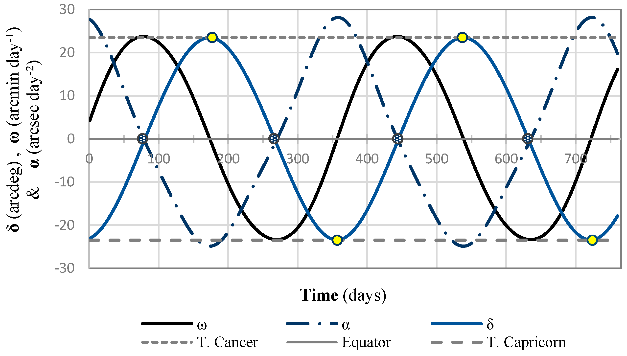
Figure 2.
Sun declination (, left) and acceleration of declination (, right) against velocity of declination (), throughout a Gregorian year.
Figure 2.
Sun declination (, left) and acceleration of declination (, right) against velocity of declination (), throughout a Gregorian year.
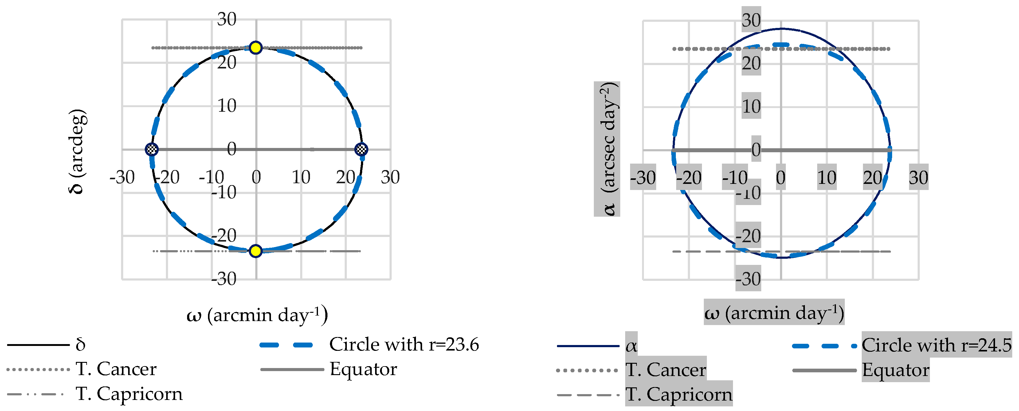
Figure 3.
Angular velocity () and angular acceleration () of the Sun meridian declination (), in association with the Equation of Time (E, minutes of time); within a Gregorian year. Equinoxes (solid circle) and solstices (open circle) are tagged on the analemma () at the three main parallels.
Figure 3.
Angular velocity () and angular acceleration () of the Sun meridian declination (), in association with the Equation of Time (E, minutes of time); within a Gregorian year. Equinoxes (solid circle) and solstices (open circle) are tagged on the analemma () at the three main parallels.
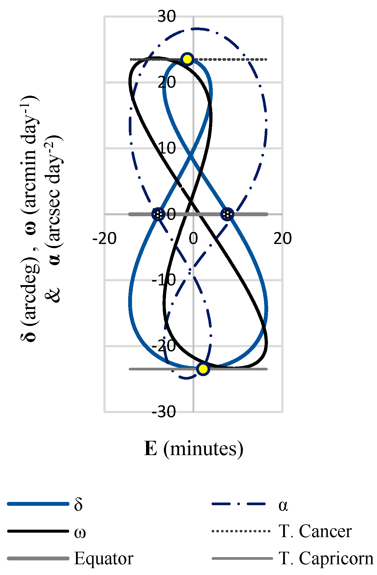
Figure 4.
Budget of natural beam irradiance ) expressed as a percentage of the budget annually available (100%) that is delivered per arcdeg of latitude, where and = 0.274 % day-1. The function is presented separately for each season (green, yellow, brown, and blue circles).
Figure 4.
Budget of natural beam irradiance ) expressed as a percentage of the budget annually available (100%) that is delivered per arcdeg of latitude, where and = 0.274 % day-1. The function is presented separately for each season (green, yellow, brown, and blue circles).
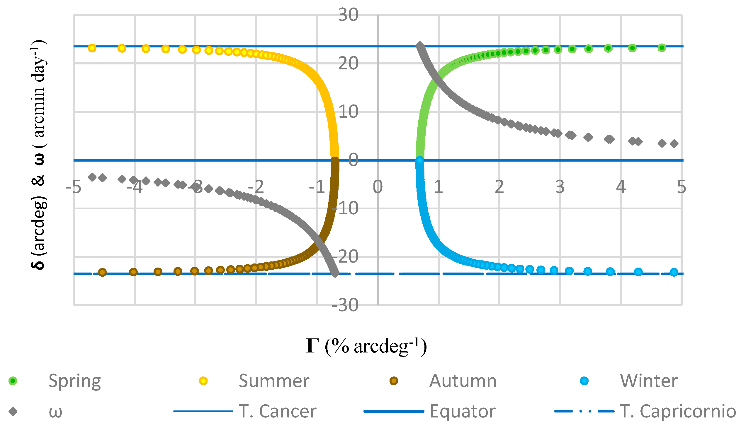

Table 1.
Angular velocity () and acceleration () of the Sun meridian declination (, as well as within season records for exposure term and the budget of natural beam irradiance attained by each of the ten arbitrary belts (), during the declination cycle.
Table 1.
Angular velocity () and acceleration () of the Sun meridian declination (, as well as within season records for exposure term and the budget of natural beam irradiance attained by each of the ten arbitrary belts (), during the declination cycle.
| Season | Belt name |
(arcdeg) |
(arcmin day-1) |
(arcsec day-2) |
Exposure term (days) | Starting date (month/day) |
(% arcdeg-1) |
| Spring | Equatorial | [+0, +5) | 23.48 | -3.00 | 11 | 3/22 | 0.60 |
| A | [+5, +10) | 22.32 | -7.38 | 15 | 4/2 | 0.82 | |
| B | [+10, +15) | 19.86 | -12.30 | 15 | 4/17 | 0.82 | |
| C | [+15, +20) | 15.74 | -17.47 | 18 | 5/2 | 0.99 | |
| Cancer | [+20, +23.5] | 6.62 | -23.27 | 34 | 5/20 | 2.66 | |
| Summer | Cancer | (+23.5, +20] | -6.59 | -23.11 | 32 | 6/23 | 2.50 |
| C | (+20, +15] | -15.41 | -17.21 | 19 | 7/25 | 1.04 | |
| B | (+15, +10] | -19.57 | -11.93 | 15 | 8/13 | 0.82 | |
| A | (+10, +5] | -21.91 | -7.36 | 14 | 8/28 | 0.77 | |
| Equatorial | (+5, +0) | -23.09 | -3.09 | 13 | 9/11 | 0.71 | |
| Autumn | Equatorial | [+0, -5) | -23.30 | 1.24 | 13 | 9/24 | 0.71 |
| A | [-5, -10) | -22.52 | 6.00 | 13 | 10/7 | 0.71 | |
| B | [-10, -15) | -20.46 | 11.66 | 15 | 10/20 | 0.82 | |
| C | (-15, -20] | -16.11 | 18.68 | 19 | 11/4 | 1.04 | |
| Capricorn | [-20, -23.5] | -6.67 | 26.11 | 30 | 11/23 | 2.35 | |
| Winter | Capricorn | (-23.5, -20] | 6.90 | 26.26 | 30 | 12/23 | 2.35 |
| C | (-20, -15] | 16.78 | 18.57 | 18 | 1/22 | 0.99 | |
| B | (-15, -10] | 20.64 | 12.24 | 15 | 2/9 | 0.82 | |
| A | (-10, -05] | 22.82 | 6.36 | 13 | 2/24 | 0.71 | |
| Equatorial | (-05 +0) | 23.64 | 1.30 | 13 | 3/9 | 0.71 |
Declination data were derived from the geometric model of solar declination (Spencer, 1971). The five belts of spring are the very same five belts of summer. .
Table 2.
Angular velocity () and acceleration () of the Sun meridian declination (, exposure and resting terms, and budget of natural beam irradiance () for each of five arbitrary belts, averaged for two hemispheres throughout a Gregorian year.
Table 2.
Angular velocity () and acceleration () of the Sun meridian declination (, exposure and resting terms, and budget of natural beam irradiance () for each of five arbitrary belts, averaged for two hemispheres throughout a Gregorian year.
| Belt |
(arcdeg) |
(arcmin day-1) |
(arcsec day-2) |
Exposure term (days) |
Resting term 1 (days) | Resting term 2 (days) |
(% arcdeg-1) |
| Equatorial | (0, 5) | 23.4 | 2.2 | 25.0 | 157.5 | 182.5 | 1.37 |
| A | [5, 10) | 22.4 | 6.8 | 27.5 | 130 | 207.5 | 1.51 |
| B | [10, 15) | 20.1 | 12.0 | 30.0 | 100 | 235 | 1.64 |
| C | [15, 20) | 16.0 | 18.0 | 37.0 | 63 | 265 | 2.03 |
| Tropical | [20, 23.5] | 6.7 | 24.7 | 63.0 | 0 | 302 | 4.93 |
| Weighted average |
15.4 | 15.4 |
involves the sum of NBI budgets for the two exposure terms on which the belt holds the NBI along the year.
Disclaimer/Publisher’s Note: The statements, opinions and data contained in all publications are solely those of the individual author(s) and contributor(s) and not of MDPI and/or the editor(s). MDPI and/or the editor(s) disclaim responsibility for any injury to people or property resulting from any ideas, methods, instructions or products referred to in the content. |
© 2024 by the authors. Licensee MDPI, Basel, Switzerland. This article is an open access article distributed under the terms and conditions of the Creative Commons Attribution (CC BY) license (http://creativecommons.org/licenses/by/4.0/).
Copyright: This open access article is published under a Creative Commons CC BY 4.0 license, which permit the free download, distribution, and reuse, provided that the author and preprint are cited in any reuse.


