
Submitted:
06 July 2024
Posted:
09 July 2024
You are already at the latest version
Abstract
This paper examines the impact of random sample sizes on the extreme value theory of competing risks, a significant area in finance and environmental science. We capture limit distributions of two extreme types under random sampling sizes, known as accelerated mixed l-max and p-max stable type distributions. The study presents results for both maxima and minima in competing risks scenarios, addressing cases of independent and non-independent random sample sizes. Numerical examples validate our theoretical findings, demonstrating the applicability of our approach to various random sample size distributions, including time-shifted Poisson or binomial, geometric, and negative binomial distributions.
Keywords:
extreme value theory
; competing risks
; random sample size
1. Introduction
Extreme Value Theory (EVT) is dedicated to modeling extreme events within a sequence of a large number of independent and identically distributed (i.i.d.) random variables. Its applications are diverse, spanning fields such as finance, insurance, environmental science, and engineering [8,14]. Let be a sequence of i.i.d. random variables with common distribution function (d.f.) F, and denote by the sample maxima. The risk is called to be in the max-domain attraction of G, if there exist some normalization constants and a non-degenerate d.f. G such that (with convergence in distribution)
The limit distribution G is the so-called generalized extreme value distribution (GEV), which is of the sample l-type (namely, x can be replaced with for some ) as
We denote this by . Here the three parameters are called the shape, location, and scale parameters, respectively. In addition, the tail behavior of the potential risk X is well classified into Fréchet, Weibull, and Gumbel domains, corresponding to the cases with , respectively [3].
Given the wide applications of EVT, many extensive studies of limit theory alike Eq.(1) have been conducted. [16] extended first the limit distribution under linear normalization in Eq.(1) to the power limit laws , i.e., there exist some power normalization constants and a non-degenerate d.f. H such that
with the sign function equal 1, and 0 for x being positive, negative and zero, respectively. It is well-known that H is of p-max stable distributions composed of six types of limits, which can be rewritten uniformly as below [15]. For some and (recall G is the GEV defined in Eq.(2)),
In what follows, we denote this by .
Recently, [5] and [12] investigated the limit behavior of extremes under linear and power normalization in the scenario of competing risks, with the practical consideration of aggregating multiple sources. Namely, the studied sample maxima is actually obtained from k heterogeneous subsamples from source/population . This considerate modeling in the big data era is desirable due to the complexity of real applications [6,24]. The limit theory of obtained for the k multiple sources is the so-called limit theory of max of max since
Clearly, the obtained limit laws of Eq.(5) extending the classical extreme value theory given in Eqs.(1) and (3) are the so-called accelerated l-max stable and accelerated p-max stable distributions, see Theorem 2.1 [5] and Theorem 2.1 [12]. Note that the key condition in determining accelerated limit theory is the interplay of the sample length and the tail behavior among the multiple competing risks. A natural question is how the extreme law varies in the uncertainty of the sample size involved. This is very common in environmental and financial fields, for instance, the extreme claim size of claims over a n-day period and the extreme daily precipitation within a duration of wet period [13,21]. This paper aims to study the limit theory under both linear and power normalization in the framework of competing risks with random sample size.
Many authors refined the extreme limit theory under linear normalization with random sample size for two different cases:
- Case I) with independent random sample size. The basic risks and sample size index are supposed to be independent and converges weakly to a non-degenerate distribution function [9];
- Case II) with non-independent random sample size. There exists a positive-valued variable V such that converges to V in probability, allowing the interrelation of the basic risk and sample size index [19].
The limit theorems with random sample size were further extended for sample minima [7], extreme order statistics under power normalization [2,18], stationary Gaussian process [22], stationary chi-process [23], and recent contributions on multivariate extreme behavior [11]. This paper will further consider the limit behavior of extremes (both minima and maxima) under linear and power normalization in the competing risk scenario, extending those accelerated l-max and p-max stable limit distributions when the sample size sequence satisfies conditions indicated in Cases I) and II). The theoretical results will be illustrated by numerical studies with typical examples such as are time-shifted Poisson, (negative) Binomial distributions, which have extensive applications in insurance and hydrology [19,20].
The remainder of the paper is organized as follows. Section 2 presents the main results for maxima of maxima under both linear and power normalization with sample sizes. Extensional results for competing minima and typical examples are discussed in Section 3. Numerical studies are conducted to illustrate our theoretical findings in Section 4. The proofs of all theoretical results are deferred to the Appendix.
2. Main Results
Notation. Recall that the max of max defined in Eq.(5), is generated from k independent samples of size ’s from risk . Let be mutually independent, positive integer-valued variables, standing for the random sample size, which is independent of the basic risks . Similar to Eq.(5), we write
Here and . Throughout this paper, for any risk X following a cumulative distribution function (cdf) F, we write , standing for the cdf of . Further, all limits are taken as .
To simplify the notation, in what follows, we consider competing risks from two sources, namely with . We will present below the limit behavior of for Cases I) and II) in Section 2.1 and Section 2.2, respectively.
2.1. Limit theorem for Case I) with independent sample size
In this section, we present our main results on the limit behavior of competing risks under linear and power normalization in Theorems 1 and 2, respectively. Basically, we focus on the following random sample size scenario: Assume that there exist independent non-degenerate distributed such that
Condition (7) is commonly used for the limit behavior of extremes with random sample size [4,18,23]. We refer to [17] for relevant examples, see also Examples 1 to 3.
Limit behavior of under linear normalization. Clearly, for , there exist such that satisfies Eq.(1) as . We will show in Theorem 1 below that, under condition (7), the limit theorem for competing extremes holds for an accelerated mixed GEV distribution with
Theorem 1.
Let be given by Eq.(6) with the basic risks and random sample sizes mutually independent. Suppose that condition (7) and holds with Eq.(2) for and . If there exist two constants and such that
as .
Here are given by Eq.(8).
Remark 1.
a) Theorem 1 is reduced to Theorem 2.1 by [5] if ’s are degenerate at one, the limit theorem for competing maxima with determinant sample size.
b) In addition, the two results in (i) and (ii) correspond to the cases for two competing risks being comparable tails and balanced sampling process and the dominated case, respectively.
Limit behavior of under power normalization. Clearly, for , there exist such that satisfies Eq.(3) as . We will show in Theorem 2 below that, under condition (7), the limit theorem for competing extremes holds for an accelerated mixed H distribution given below
Theorem 2.
Let be given by Eq.(6) with the basic risks and random sample sizes mutually independent. Suppose that condition (7) and holds with Eq.(3) for and . If there exist two non-negative constants α and β such that
as . The following claims hold for , the mixed distributions defined in Eq.(10).
- (i).
- If condition (11) holds with two positive constants α and β, then
- (ii).
-
The following limit distribution holdsprovided that one of the following four conditions is satisfied (notation: , the right endpoint of )
- a).
- When is one of the same p-types of , and is one of the same p-types of .
- b).
- When is one of the same p-types of , and is one of the same p-types of for . In addition, Eq.(11) holds with and .
- c).
- When is one of the same p-types of , and is the same type of for . In addition, Eq.(11) holds with and or and .
- d).
- When both and are one of the same p-types of . In addition, Eq.(11) holds with and or and .
Remark 2.
a) Theorem 2 is reduced to Theorem 2.1 by [12] if ’s are degenerate at one, which means the asymptotically almost randomlessness of , the limit theorem for competing maxima with determinant sample size. This situation happens in practice, e.g., follows a shifted Poisson df with mean such that . For more examples, see Example 1 below and Remark 2.2 by [1].
b) In addition, the two results in i) and ii) correspond to the two different cases with and in condition (11), illustrating the limit behavior of two competing risks with comparable tails and balanced sampling process and the dominated case, respectively.
2.2. Limit theorem for Case II) with non-independent sample size
In this section, we focus on Case II), relaxing the independent condition between the basic risk and random sample size. On the other hand, we need to strengthen the convergence in distribution as the convergence in probability, as stated below. Assume that there exist positive random variables such that (notation: stands for convergence in probability)
Theorem 3.
3. Discussion
In this section, we first extend our results for competing minima risks in Section 3.1, and then present typical examples of random sizes with specific mixed extreme distributions in Section 3.2.
3.1. Extreme Limit Theory for Competing Minima Risks
In some practical applications, such as the lifetime in reliability analysis or race time of athletes in physical studies, extreme minima plays an important role. As we will see in Corollaries 1 and 2 below, analytical claims follow for competing risks with random sample size in terms of minima of minima. Essentially, noting that the right tail behavior of is demonstrated by its sample maxima , the left tail behavior of can be shown by the sample minima since (cf. see Theorem 1.8.3 [14] and [10])
Noting that, the condition that , i.e., there exist such that satisfies Eq.(1) as , is equivalent that
where is of the same l-type of GEV distribution given in Eq.(2).
Corollary 1.
Suppose the same conditions as for Theorems 1 or 3 are satisfied.
Here are given by Eq.(8).
Noting that , the following corollary holds for the power normalized minima of minima.
Corollary 2.
Suppose the same conditions as for Theorems 2 or 4 are satisfied. The following claims hold for with the mixed distributions defined in Eq.(10).
- (i).
- If condition (11) holds with two positive constants α and β, then
- (ii).
-
The following limit distribution holdsprovided that one of the conditions a)∼ d) in Theorem 2 holds.
Remark 3.
a) Recalling that G and H given by Eqs.(2) and (4) are the so-called l-max stable and p-max stable, we call L and P the mixed accelerated l-max stable and the mixed accelerated p-max stable distributions if they can be written as a product of and , respectively.
b) Recalling that the and are the so-called l-min stable and p-min stable distributions [Corollary 1 [10] if G and H are given by Eqs.(2) and (4), we call and the mixed accelerated l-min stable and the mixed accelerated p-min stable distributions if they can be written as a product of and , respectively.
3.2. Examples
Below, we will give three examples to illustrate our main results obtained in Theorems 1 and 2. In particular, we considered that random sample size follows respectively time-shifted version of Poisson or binomial distribution, geometric and negative binomial distributions with relevant parameters satisfying certain average stable conditions [17], see Examples 1 ∼ 3.
Example 1
(Time-shifted binomial/Poisson distributed random sample size). Let follow a time-shifted binomial distribution with probability mass function (pmf) given as
If , then converges in probability to one. Similarly, for a time-shifted Poisson distributed with , then converges in probability to 1 [Lemmas 4.3 [17]. For the random sample size aforementioned, the claims of Theorems 1 and 2 follow as the reduced determinant random size cases, see Remarks 1(a) and 2(a).
Example 2
(Time-shifted geometric distributed sample size). In the case of linear normalization, with G being one of the three l-types distribution, say specified in Eq.(2). Suppose that the random sample size follows a geometric distribution with mean . We have in distribution with a random scale V following a standard exponential distribution. Consequently, Theorem 1 holds with an accelerated mixed l-max stable distribution L, the product of mixed l-max stable distributions of form L as below.
which is taken as its limit for .
Example 3
(Time-shifted negative binomial distributed sample size). As an extension of m-shifted geometric distributions, we consider time-shifted negative binomial distributed sample size with given by
It follows by Lemma 4.1 by [17] that, as , we have converges in distribution to V, a gamma random variable with shape parameter r and scale parameter 1, i.e., the cdf of V is given by
where denotes the gamma function. It follows by Theorem 1 that
Similarly, Theorem 2 follows with the accelerated mixed p-max stable distributions, the product of form P given below.
4. Numerical Studies
We will conduct a Monte Carlo simulation to illustrate Theorems 1 and 2 with m-shifted random sample size given in Examples 2∼1. In what follows, we take the shift parameter in all time-shifted random sample size distributions, and the basic risks from Pareto distributions with parameters 1 and the random sample sizes are supposed to be mutually independent. In addition, the repeated time is taken as . We will illustrate our main results specified in Theorems 1 with the three examples given in Section 3.2 above.
1. Comparison of Pareto competing extremes with determinant sample size and Poisson distributed random sample size.
In Figure 1, we will demonstrate that the competing extremes with Poisson distributed sample size are similar to the case with nonrandom sample size case. Let follow m-shifted Poisson with mean parameters . We then generate competing Pareto extremes with basic risks following Pareto with It follows from Theorems 1, 2 and Example 1 together with Example 4.6 by [12] that (recall the Fréchet distribution)
- (1)
- For or with , we have
- (2)
- For with , we have
Noting that the power normalized extremes will behave similarly to the linear normalized ones up to a power transformation. We show only the behavior of linear normalization for the numerical studies below.
In Figure 1, we take and with to show the above two cases. Overall, the competing Pareto extremes are well fitted by the accelerated GEV distribution for the non-randomized sample size, where the latter is slightly better than the randomized sample size cases. Further, the accelerated GEV approximation (Figure 1 (a, c)) is relatively closer to the empirical competing extremes than the dominated case.
2. Comparison of Pareto competing extremes with Geometric distributed and negative Binomial distributed sample size. We consider the max of maxima with both basic risks with random sample size following m-shifted negative Binomial distribution with probability and . It follows by Example 4.6 by [12], Theorem 1(a, b) and Example 3 that, with
- (1)
- For or with , we have
- (2)
- For with , we have
Thus, its density function is given by
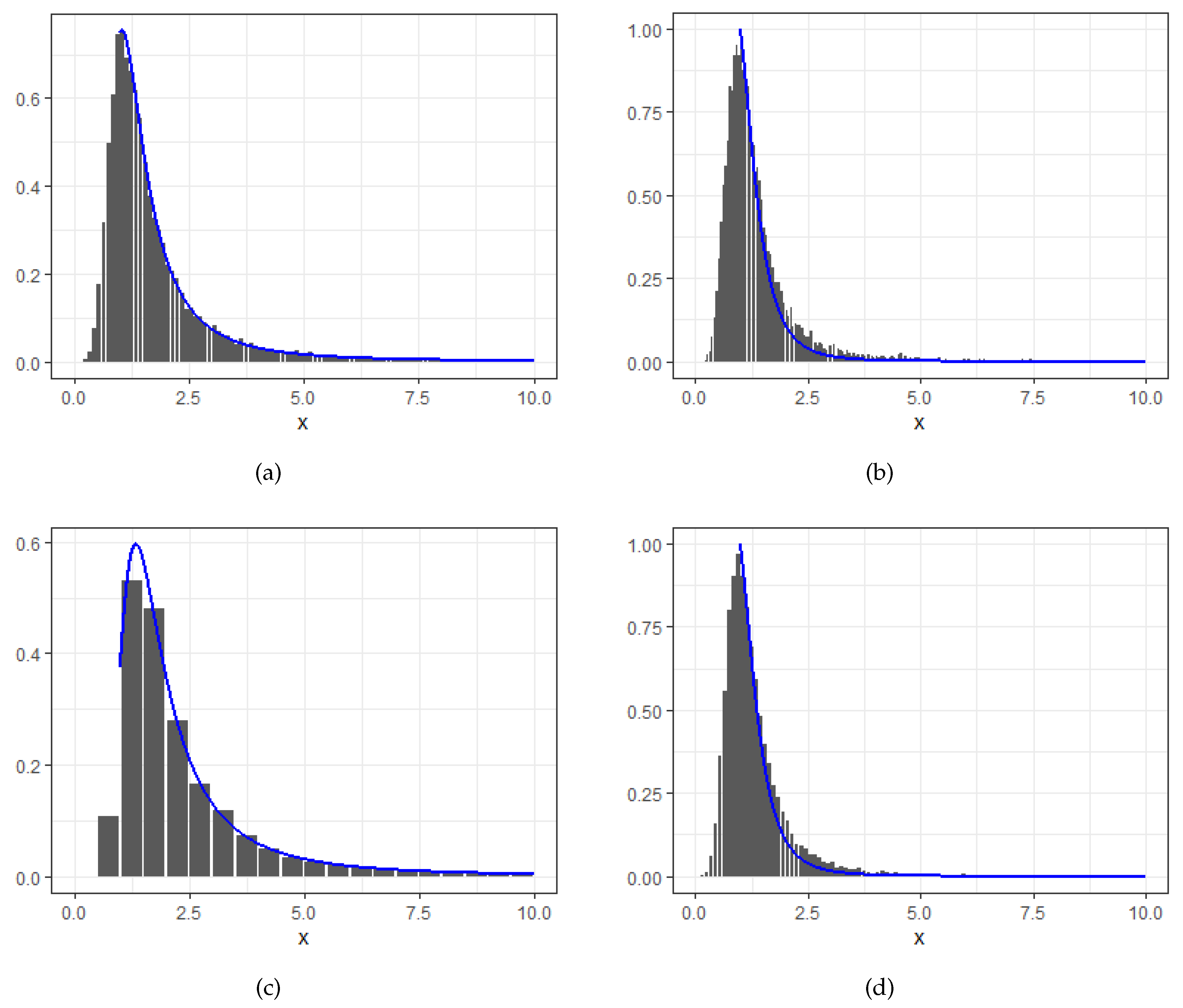
In Figure 2, we set with in (a, c) and (b, d), respectively. Meanwhile, the random sample size follows a 5-shifted negative Binomial distribution with in (a, b) (namely geometric distribution), and in (c, d), and successful probability . Meanwhile, we take in the Pareto basic risks. Consequently, the sub-maxima are completely competing when , resulting in the accelerated mixed extreme limit distributions as shown in Figure 2 (a, c). In contrast, the dominated limit behavior is given in Figure 2 (b, d) as .
In general, our theoretical density curve given by Eq.(16) approximates the histogram very well (Figure 2). Further, we see that the approximation with geometric distributed random size is slightly better than the negative binomial case. In addition, the approximation for the dominated case (Figure 2 (d)) is slightly better than the accelerated case when negative Binomial random size applies.
Author Contributions
Conceptualization, L.B., K.H. and C.L.; Methodology, K.H. and C.L.; software, L.B.; validation, L.B., Z.T. and C.L.; formal analysis, L.B., K.H. and C.L.; investigation, K.H.; Writing, original draft preparation, C.L. and K.H.; Writing, review and editing, C.W., Z.T. and C.L.; Visualization, C.L.; Supervision, C.L.; Project administration, C.L.; Funding acquisition, C.L. All authors have read and agreed to the published version of the manuscript.
Funding
Long Bai is supported by National Natural Science Foundation of China Grant no. 11901469, Natural Science Foundation of the Jiangsu Higher Education Institutions of China grant no. 19KJB11002 and University Research Development Fund no. RDF-21-02-071. Chengxiu Ling is supported by the Research Development Fund [RDF1912017], and the Post-graduate Research Fund [PGRS2112022] at Xi’an Jiaotong-Liverpool University.
Institutional Review Board Statement
Not applicable.
Informed Consent Statement
Not applicable.
Data Availability Statement
Not applicable.
Acknowledgments
We thank the editors and all reviewers for their constructive suggestions and comments that greatly helped to improve the quality of this paper.
Conflicts of Interest
The authors declare no conflict of interest.
Appendix A Proofs of Theorems 1 ∼ 4
Proof of Theorem 1. It follows by the independence between the basic risks and the random sample size , and condition (1) holding for that
Further, it follows by the mutual independence between and that
The straightforward application of Eq.(A2) gives
Similarly, we rewrite as
We complete the proof of Theorem 1.
Proof of Theorem 2. Firstly, we rewrite the left-hand side of Eq.(12) as follows.
It follows by Theorem 2.1 in [2] that
Next, we show the limit of . We rewrite as
where with given by Eq.(11). The remaining proof is similar to those for Theorem 2.1 by [12]. We complete the proof of Theorem 2.
Proof of Theorem 3 It follows by Theorem 6.2.1 of [9] that, for the jth sample maxima , when the constant sequences such that (1) holds, and satisfies Eq.(7), we have the claim in Eq.(A1). The remaining proofs follow by those for Theorem 2.1 by [5].
Proof of Theorem 4 We show first that, the claim follows for the jth sample maxima with the constant sequences , i.e.,
Denote by the probability mass function of . We have
It follows by the total law of probability and the independence between basic risks and sample size that
Since as , we have . Therefore,
Noting that condition (7) implies that, there exists a sub-sequence such that . It follows thus from Theorem 2.1 by [4] that, for every ,
Consequently, we obtained the claim (A6).
References
- Abd Elgawad, M., Barakat, H., Qin, H., and Yan, T. (2017). Limit theory of bivariate dual generalized order statistics with random index. Statistics, 51(3):572–590. [CrossRef]
- Barakat, H. and Nigm, E. (2002). Extreme order statistics under power normalization and random sample size. Kuwait Journal of Science & Engineering, 29(1):27–41.
- Beirlant, J. and Teugels, J. L. (1992). Limit distributions for compounded sums of extreme order statistics. Journal of Applied Probability, 29(3):557–574. [CrossRef]
- Berman, S. M. (1962). Limiting distribution of the maximum term in sequences of dependent random variables. The Annals of Mathematical Statistics, 33(3):894–908.
- Cao, W. and Zhang, Z. (2021). New extreme value theory for maxima of maxima. Statistical Theory and Related Fields, 5(3):232–252. [CrossRef]
- Cui, Q., Xu, Y., Zhang, Z., and Chan, V. (2021). Max-linear regression models with regularization. Journal of Econometrics, 222(1, Part B):579–600. [CrossRef]
- Dorea, C. C. and GonÇalves, C. R. (1999). Asymptotic distribution of extremes of randomly indexed random variables. Extremes, 2(1):95–109.
- Embrechts, P., Kluppelberg, C., and Mikosch, T. (1997). Modelling Extremal Events. Stochastic Modelling and Applied Probability. Springer, Heidelberg.
- Galambos, J. (1978). The Asymptotic Theory of Extreme Order Statistics. Wiley series in probability and mathematical statistics. Wiley, New York.
- Grigelionis, B. (2004). On the extreme-value theory for stationary diffusions under power normalization. Lithuanian Mathematical Journal, 44:36–46. [CrossRef]
- Hashorva, E., Padoan, S. A., and Rizzelli, S. (2021). Multivariate extremes over a random number of observations. Scandinavian Journal of Statistics, 48(3):845–880.
- Hu, K., Wang, K., Constantinescu, C., Zhang, Z., and Ling, C. (2023). Extreme limit theory of competing risks under power normalization. arXiv: 2305.02742.
- Korolev, V. and Gorshenin, A. (2020). Probability models and statistical tests for extreme precipitation based on generalized negative binomial distributions. Mathematics, 8(4):604. [CrossRef]
- Leadbetter, M. R., Lindgren, G., and Rootzén, H. (1983). Extremes and related properties of random sequences and processes. Springer Science & Business Media.
- Nasri-Roudsari, D. (1999). Limit distributions of generalized order statistics under power normalization. Communications in Statistics - Theory and Methods, 28(6):1379–1389.
- Pantcheva, E. (1985). Limit theorems for extreme order statistics under nonlinear normalization. Springer Berlin Heidelberg.
- Peng, Z., Jiang, Q., and Nadarajah, S. (2012). Limiting distributions of extreme order statistics under power normalization and random index. Stochastics, 84(4):553–560. [CrossRef]
- Peng, Z., Shuai, Y., and Nadarajah, S. (2013). On convergence of extremes under power normalization. Extremes, 16(3):285–301. [CrossRef]
- Ribereau, P., Masiello, E., and Naveau, P. (2016). Skew generalized extreme value distribution: Probability-weighted moments estimation and application to block maxima procedure. Communications in Statistics-Theory and Methods, 45(17):5037–5052. [CrossRef]
- Shi, P. and Valdez, E. A. (2014). Multivariate negative binomial models for insurance claim counts. Insurance: Mathematics and Economics, 55:18–29. [CrossRef]
- Soliman, A. A. (2000). Bayes prediction in a Pareto lifetime model with random sample size. Journal of the Royal Statistical Society. Series D, 49(1):51–62. [CrossRef]
- Tan, Z. and Wu, C. (2014). Limit laws for the maxima of stationary chi-processes under random index. Test, 23(4):769–786. [CrossRef]
- Tan, Z. Q. (2014). The limit theorems for maxima of stationary Gaussian processes with random index. Acta Mathematica Sinica, 30(6):1021–1032. [CrossRef]
- Zhang, Z. (2021). Five critical genes related to seven COVID-19 subtypes: A data science discovery. Journal of Data Science, 19(1):142–150. [CrossRef]
| 1 | The cdf of Pareto is given as . |
Figure 1.
Distribution approximation of linear normalized (a, b) and (c,d) with both ’s from Pareto and Poisson distributed sample size with mean . Here and with in (b,d) and (a,c) by and , respectively.
Figure 1.
Distribution approximation of linear normalized (a, b) and (c,d) with both ’s from Pareto and Poisson distributed sample size with mean . Here and with in (b,d) and (a,c) by and , respectively.
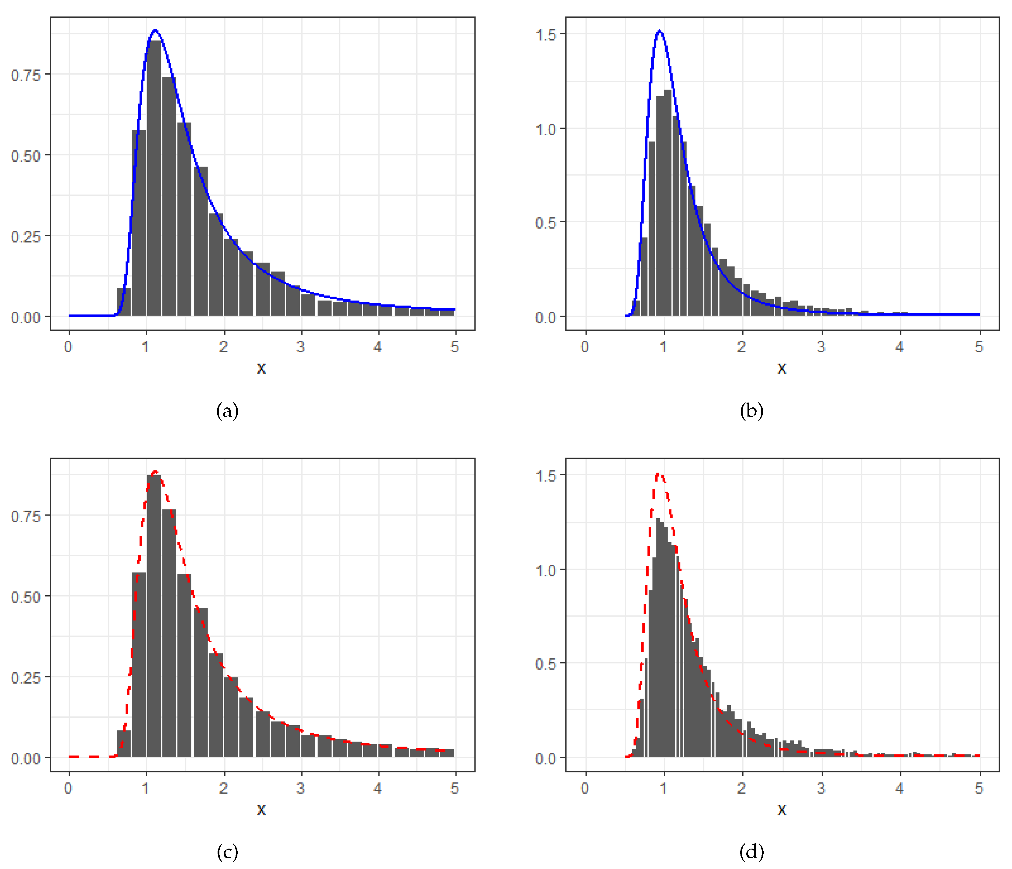
Figure 2.
Distribution approximation of linear normalized with both ’s from Pareto. The random sample size follows a negative Binomial distribution with (the geometric distribution) (a,b) and (c, d) and successful probability . Here and with in (a, c) and (b, d) with pdf curves of and , respectively.
Disclaimer/Publisher’s Note: The statements, opinions and data contained in all publications are solely those of the individual author(s) and contributor(s) and not of MDPI and/or the editor(s). MDPI and/or the editor(s) disclaim responsibility for any injury to people or property resulting from any ideas, methods, instructions or products referred to in the content. |
© 2024 by the authors. Licensee MDPI, Basel, Switzerland. This article is an open access article distributed under the terms and conditions of the Creative Commons Attribution (CC BY) license (http://creativecommons.org/licenses/by/4.0/).
Copyright: This open access article is published under a Creative Commons CC BY 4.0 license, which permit the free download, distribution, and reuse, provided that the author and preprint are cited in any reuse.


