Developing Construction Labor Productivity Model for Concreting Activity Using Artificial Neural Networks

There are various modeling techniques adopted for predicting the labor productivity that incorporate the influence of various factors, but neural networks are found to have strong pattern recognition and higher accuracy to get reliable estimates. To develop a construction labor productivity (CLP) model for concreting activities, data were collected through a questionnaire. The most critical influencing parameters were ranked according to their relative importance index (RII). Then the strength of the relationship between CLP and influencing parameters was analyzed using correlation coefficient results generated in Python program. Finally, the CLP model which represents the output of the crew within a certain factor was successfully developed using artificial neural networks (ANNs). Five objectives and six subjective critical influencing parameters were selected using RII. Crew experience, age of workers, and placement technique are the top three influencing parameters that have a strong relation with CLP with correlation coefficient values of 0.5681, 0.5349, and 0.5227 respectively. The developed model within these influencing parameters has a higher capability to predict the output of labor with a 92% coefficient of determination (R2) and a mean squared error of 0.316%. Therefore, the application of such a model for the accurate estimation of labor productivity is recommended.

Keywords:

Subject: Engineering - Civil Engineering

1. Introduction

Productivity is a key element in determining the success and failure of any construction project [1,2,3,4,5]. The most common construction productivity metrics are unit rate (ratio of labor cost to units of output); labor productivity (ratio of work hours to units of output); and productivity factor (ratio of scheduled or planned to actual work hours) [6,7]. The efficiency of activity level systems, focusing on the labor resource of the construction process, is measured using construction labor productivity (CLP). Because of different ways of defining CLP, arriving at a common definition of productivity is a puzzling task. However, many authors agree that, productivity is a quantitative assessment of the correlation between the number of resources used and the amount of output produced, therefore, it is a component of cost and is not a method of estimating the cost of resources [8,9,10].

In developing countries, labor counts for 30-50% of total project cost due to the scarce of modern construction equipment and the construction operations are largely labor-intensive [11]. Therefore, the project’s success is greatly influenced by the labor’s productivity. The performance of the construction industry is best described by its construction labor productivity, but most construction projects fail to correctly imitate the construction labor productivity, this failure is mainly due to the lack of appropriate estimation models which are very crucial for the industries overall performance.

The construction industry is searching for ways to improve labor productivity, but the industry has lacked crew-level CLP models capable of explaining which parameters cause productivity to change and by how much [12,13].Despite its importance in construction project management, developing accurate and interpretable CLP models for analysis and improvement of construction productivity has not been fully achieved[14,15].

In order to estimate construction projects in a reliable and accurate way, the help of advanced modelling techniques is vital[16]. Deferent modelling techniques like action response models, statistical model, linear regression model, and others have been prepared in past decades [2,17]. However, these modeling approaches were basically developed for specific circumstances and their implementation was restricted [17].Hence, developing the most accurate and powerful model is the current hot topic for researchers and practitioners.

In the construction industry particularly in developing countries, there is a lack of well-developed CLP models which are capable of explaining which parameters cause productivity to change and by how much, therefore the industry is searching for ways to improve labor productivity [12].Furthermore, labor productivity values are below the benchmark, which causes the risk of delay in the overall project [4,9,18]. Lack of having developed CLP model increases the uncertainty of the construction projects which intern decreases the success, profitability, and competitiveness of the company. In spite of this, there lack research initiation in developing countries to develop CLP estimation models which are very critical and important for the success of construction projects in the country. Therefore, in order to fill this research gap and to enhance the profitability, income, and competitiveness of the construction projects current studies will focus on construction stakeholders in Ethiopia.

Several researchers [19,20,21,22,23,24,25] have applied ANN’s in construction management, mostly for decision-making, forecasting, and optimization. ANN is a technique for Artificial Intelligence (AI) programs and one of the most common approaches to machine learning. These programs invest learning capabilities in intelligent systems that can improve their performance over time [26].

So, the aim of this study was to develop a construction labor productivity estimation model using ANNs for concreting activities in building construction projects located in Addis Ababa city, Ethiopia.

2. Materials and Methods

To achieve the objective of the study, a literature review on past studies on labor productivity was reviewed. From the review, numerous factors affecting the CLP at site are identified and grouped in to subjective and objective variables. Then it was distributed in form of questioner to the respondents. Using relative importance index (RII) eleven most critical influencing factors (five objective and six subjective) were identified.

The data which was collected by direct observation from the active building construction sites, which were on concreting stage was first systematically arranged in an excel spread sheet and imported into a programming software for further analysis and modeling. The correlation coefficient of these factors was calculated and used to investigate the strength of relationship between the identified most critical factors. The identified factors are used as input parameter for the model.

2.1. Model Development

Python 3.7 version has been used to develop the ANN model. The code used to develop this model was written in the Jupyter notebook and analyzed and modeled by using different Anaconda libraries for mathematical computations and visualizations.

In developing the construction labor productivity model, all data collected from direct observation are converted to numeric values on an excel spreadsheet and saved in the CSV format. The second step followed was importing the data frame into the Jupyter notebook and preprocessing the data, which involves removing duplicates and no values in the data frame. Moreover, data cleaning involves splitting the data set into two separate data sets: the first columns as the output data set, CLP, and the reaming columns as the input data set. The output data set contains the CLP collected from the construction sites and converted into the crew's output performing the concreting activity in cubic meters per hour. The input data set contains all the inputs or parameters that bring together a certain number of outputs.

Some features have an order of magnitude larger than others and unlikely these features are significantly more correlated than others to the outputs. Therefore, to avoid this over correlation, data scaling was performed in python program using the min-max scaler data normalization technique. In this study, the given dataset was scaled between 0.1 and 0.9.

2.2. Mathematical Steps for the Training Algorism into ANN’s

The systematic steps, with equations, for the workflow in an ANN through the forward and backward propagation can be set out as follows:

The first step is: the preparation, preprocessing, and scaling of data. Set all the weights and threshold levels of the network to random numbers, uniformly distributed inside a small range [27]. The data preprocessing stage is necessary to facilitate network training which can then perform preliminary processing on the data, in order to make the data easier for the neural network training to extract the relevant information [28].

Data scaling is one of the important procedures for preprocessing the data in NNs. The significant reason for data scaling is to equalize the importance of variables, to improve the training of the neural network, and to avoid the slowing down of the learning rate near the edges of specifically the output range due to the property of the sigmoid function, which is asymptotic to values 0 and 1 for logistic function (sig), for this function the scaling ranges between 0.1 to 0.9, and the linear scaling. The network’s task is made much easier and more expressive if it is provided with data scaled in a way that helps to maintain all weights within a small set of predictable ranges. Furthermore, it is a standard practice to normalize the inputs before applying them to the artificial neural network. Initializing the neural network weights to tiny random values ensures that the product of the input weight will be small [28].

In the second step, the input vector (data or signal) is presented to the input layer, which computes the input to the hidden layer by applying inputs (X₁, X₂, X₃…., X_P) for each iteration, and desired outputs (Y_d1, Y_d2, Y_d3….,Y_dp) for each iteration, to calculate the actual outputs of the neurons in the hidden layer ( y_j^q ) as shown on Equation 1:

{Y_{j}}^{q} (I) = s i g m o i d [\sum_{i = 1}^{p} X_{i} (I) . w_{i j} (I) + θ_{j}]

(1)

Where:

Y_j^q: the actual outputs of the neurons in the hidden layer for each iteration,

X_i: the value of the input parameter i for each iteration,

W_ij: the weight of input i

P: the number of neuron j in the hidden layer, and

θ_j: the threshold applied to the neuron (i.e., bias function of the hidden layer).

Third Step: The hidden layer takes its input for neurons from Equation 1 and uses it as the argument for a sigmoid function to produce the actual output of the neurons in the output layer (ykr) as shown on Equation 2.

{Y_{j}}^{r} (I) = s i g m o i d [\sum_{i = 1}^{q} X_{j k} (I) . w_{j k} (I) + θ_{k}]

(2)

Where:

Y_kr: the actual outputs of the neurons in the output layer for each iteration,

X_jk: the value of output parameter I for a hidden layer for each iteration,

W_jk: the weight of input j to the output layer,

q: the number of neuron k in the output layer, and

θ_k: the threshold applied to the neuron (i.e., bias function of output layer).

Sigmoid: the sigmoid activation function

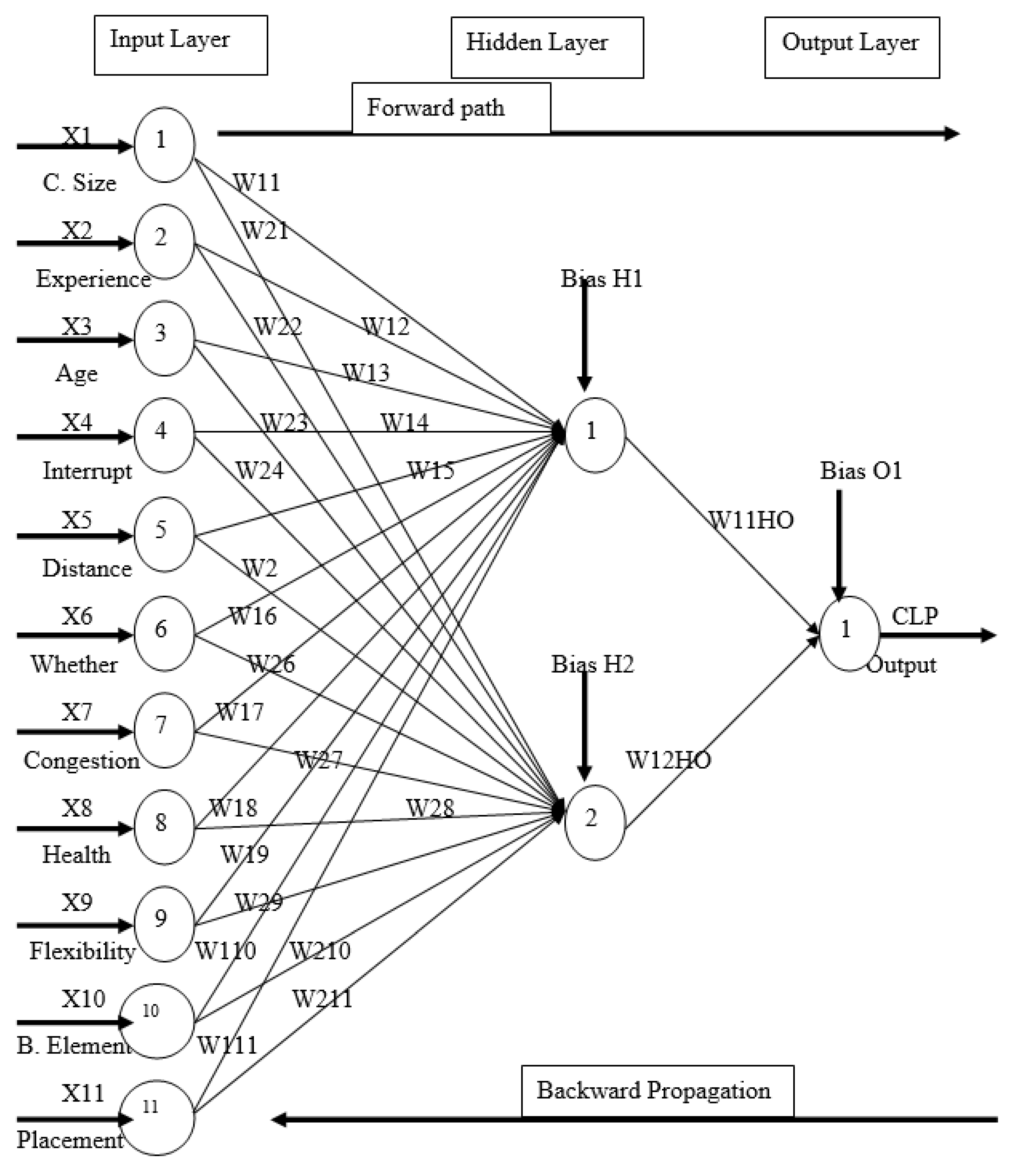
Step 4: The procedure of backward propagating the error associated with output neurons to modify the weight parameter in the back-propagation network as shown on Figure 8. The error gradient and weight correction are thereby computed for the neurons in the output layer, and then in the hidden layer. After executing Equation 3, one iteration of the training algorithms is completed. The next stage is a return to step 2 and a repetition of all the succeeding steps in the process until the detected error criterion is satisfied, or the error values remain minimum.

w_{i j} (I + 1) = w_{i j} (I) - ∆ w_{i j} (I)

(3)

Where:

ΔW_ij(I): The weight correction for the input layer with hidden layer,

Δw_jk(I): The weight correction for the hidden layer with output layer,

α: learning rate,

I: the number of iterations.

Modeling of CLP using ANN involves input, hidden, and output layers. Construction labor productivity is considered as an output layer, which shows how much product is produced by using different inputs (materials, energy, equipment, etc.) to produce outputs (project products). The hidden layer is a nonlinear combination of the network inputs that are computed. A sigmoid function was used in the program which represents the nonlinear function.

3. Results

3.1. Identification of input Parameters

As discussed in shown on Table 1. and summarized in appendix 1 numerous input parameters that can influence CLP have been identified from the review of the literature. The identified 30 context-specific factors were grouped under two main categories: 12 objective (quantitative) and 18 subjective (qualitative) variables. A questionnaire survey was conducted in Addis Ababa City construction sites with 32 respondents from project managers, contractors, consultants, masons, and foremen to identify the most critical factors from the identified 30 factors and consequently to establish a top 11 factors: 5 objective and 6 subjective factors. The summary of PI for all factors is summarized in Table 1, and Figure 1.

Table 1 show the twelve quantitative and eighteen qualitative variables which were identified by a critical review of numerous published documents, reports, records, and books. Those factors which can cause variation in productivity on a daily basis or in the short term are the primary selection criteria that were adopted to select context-specific parameters.

Figure 1 shows the ranking of the most critical factors influencing CLP. A crew size or a number of workers was ranked 1st from identified context-specific factors that can influence CLP, with an RII value of 0.913. Crew size has a great influence on productivity. This result is supported by [1,29] who found that the crew size affects labor productivity.

The health status of workers ranked 2^nd to affect construction labor productivity with an RII value of 0.888. The health status of workers is one of the most important parameters to affect CLP. This finding is supported by [30]. Distance from temporary material storage to casting place was found to be the 3^rd most critical factor that can influence CLP with an RII value of 0.875. According to [12], the final placing distance to the material mixing distance can affect CLP. Transporting the mix to the final casting place requires considerable time which consequently affects productivity.

3.2. Quantification of Input Parameters

Quantification of input parameters (independent variables) is the vital and starting point for the analysis and modeling of CLP studies. The quantification of parameters is complicated since they are a mix of objective and subjective variables. Therefore, quantification requires proper and understandable measurement schemes. For each identified most critical factors a measurement scale that is used to data collection must be developed, so as to quantify the input parameters and simplifies the construction site data collection process. The quantification in this research is done for all parameters as shown in Table 2.a and 2.b

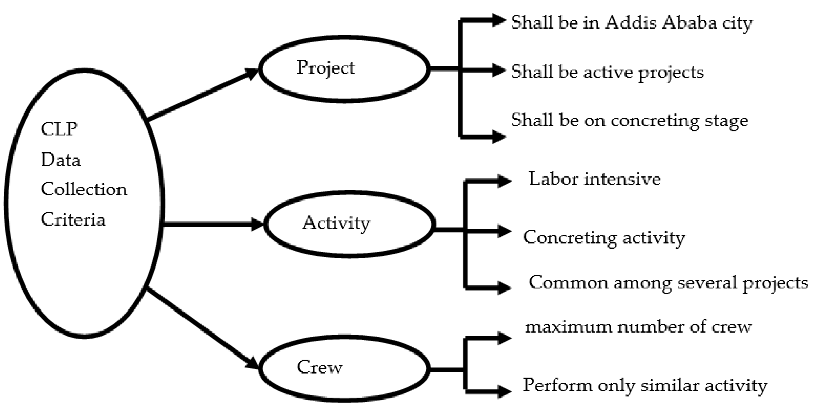
Data can be gained from the following sources: researcher (data collector), foreman, and crew members), these data sources would be assigned to each parameter and sub-parameter based on the respondent’s knowledge about the source of data in question. Data that can be collected by direct observation like weather conditions can be collected by the researcher or DC. For this research, the preferred criterion for direct observation data collection is summarized as shown in Figure 2.

Table 2. a: Input parameters for objective variables.

In put parameters for objective Variables
Identification code.	Parameter	Description	Measurement scale (unit)	Data source
N	Crew Size (number of workers)	Weather condition (comfort level)	Integer	DC*
E	Crew experience (seniority)	The average years of experience of the crew members in concreting activity	Real number	F+CM*
A	Age of workers	The average age of workers performing the actual work in years.	Real number	F+CM*
I	Level of interruption and disruption	The time lost and delayed events are caused due to several reasons, which may disrupt the crew from performing the assigned tasks.	Integer (total minutes spent)	DC
D	Distance from mixing place to final casting and finishing place	The average distance between mixing place to final placing and finishing	Integer	DC

Table 2. b: Input parameters for subjective variables.

In put parameters for subjective variables
Identification Code.	Parameter	Description	Measurement scale (unit)	Data source
W	Whether condition	The atmospheric weather condition of the site during performing the required task	1-4 pre-determined rating shown below 1- Sunny 2- Moderately sunny 3- Moderately rainy 4- Rainy	DC
C	Congested work area	Arrangement of falsework and ease of the site to perform the task in question	1-4 pre-determined rating shown below 1- Completely uncongested 2- Somewhat congested 3- congested 4- completely congested	DC
H	Health status of workers	Health status of workers during the execution of the task	1-4 pre-determined rating shown below 1- Very good 2- Good 3- Moderate 4- Bad	CM
F	Crew flexibility	Crew willingness in performing other members’ task	1-4 pre-determined rating shown below 1- Completely willing 2- Willing 3- Somewhat willing 4- Completely unwilling	DC
B	Building element	Beam, column, slab, septic tank	1-4 pre-determined rating shown below 1- Slab 2- Beam 3- Column 4- Septic tank	DC
P	Placement technique	Pump, winch, bucket, direct chute	1-4 pre-determined rating are shown below 1- Pump 2- Winch 3- Direct chute 4- Bucket	DC

* DC=data collector, F= foreman, and CM= crew member.

3.3. Data Analysis

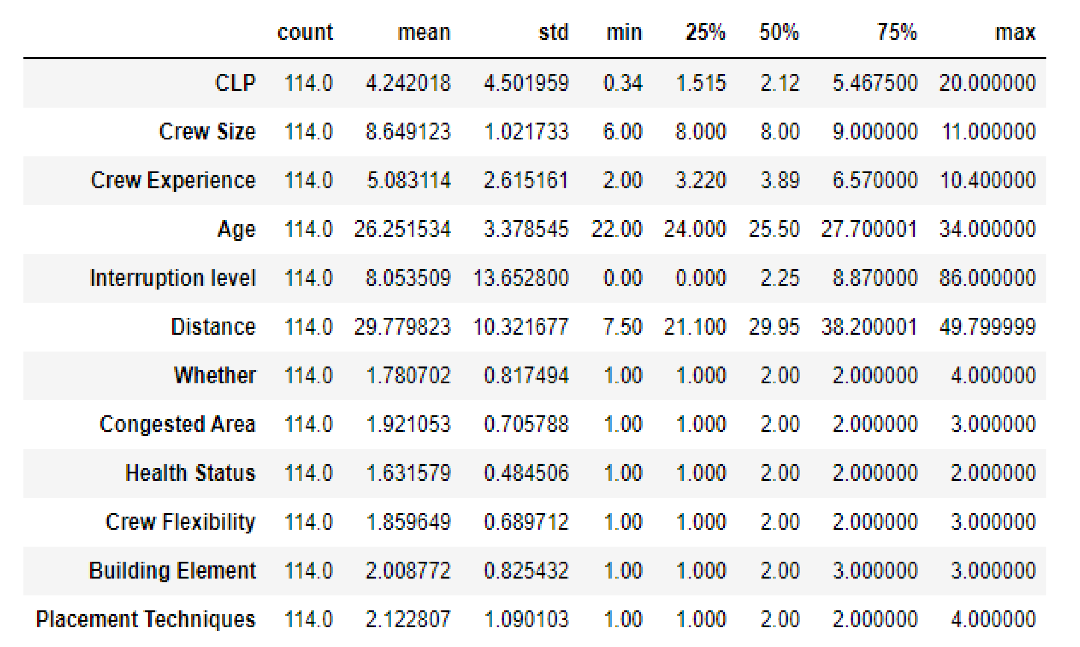
All the data collected by direct observation from the construction site are first tabulated and saved in CSV format in an excel spreadsheet and then imported into Python. The descriptive statics of the collected data were shown in Table 3 which can clearly show the summary of the collected dataset.

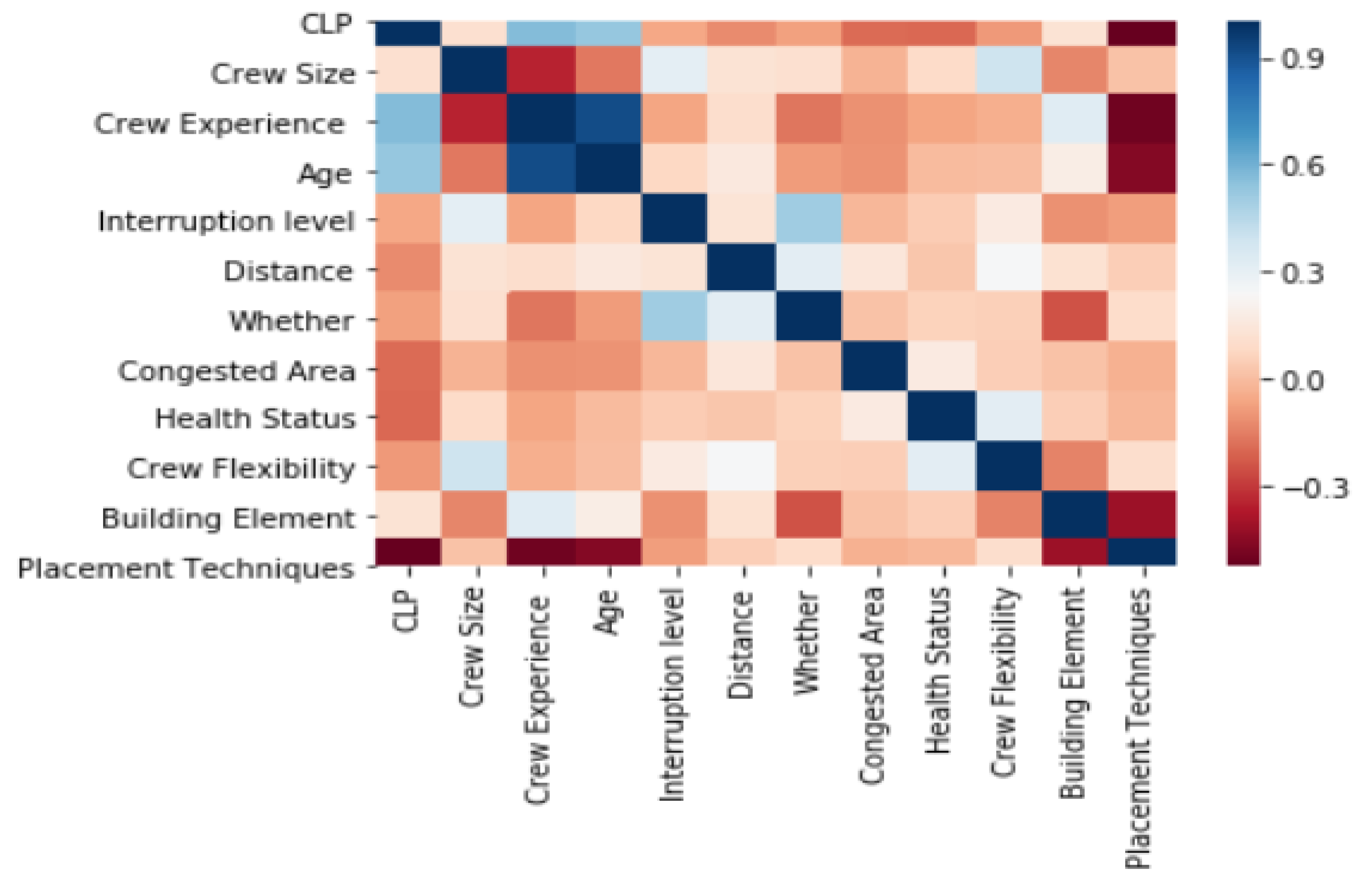
To measure the strength of the relationship between construction labor productivity and its critical influencing factors and between the independent variables a correlation coefficient was calculated using python 3.7 as shown in Table 4. The correlation coefficient shown in Table 4 is computed by considering the construction labor productivity rate of concreting activity as “Y” and its all-critical influencing factors as “X”. The values show the strength of a linear relationship of collected data between CLP and its influencing factors. If the sign of the R is positive, the value of CLP increases when influencing factors increase. If the sign is negative CLP decreases as the influencing factor increases.

In Figure 3 it is clearly observed that strongly correlated factors have dark red and dark blue colors whereas, the strength of the relationship between variables decreases as the colors contrast decreases. Along the diagonal, it is shown that everything is perfect dark blue this is because along the diagonal correlation is 1, which is the correlation of variables with itself.

3.4. Optimal Data Division

The CLP model was developed on all 114 data instances collected through direct observation. This dataset was divided into training, validation and test data sets for the purpose of accurate modeling and for testing the performance of the model. The best data allocation for this problem is shown in Table 5. This optimal number of data divisions was obtained by trial and error. Data was divided into different training, validation, and testing data divisions and observed their performance. Therefore, the data division shown in the table performs best than other data division with less error and high convergence.

3.5. ANN Optimal Parameters

Table 6 shows the optimal model development parameters. Most of this multi-layer’s perceptron (MLP) parameters were obtained by trial and error after comparisons of the performance of the model.

3.5.1. Effects of Hidden Nodes on Performance of NN’s

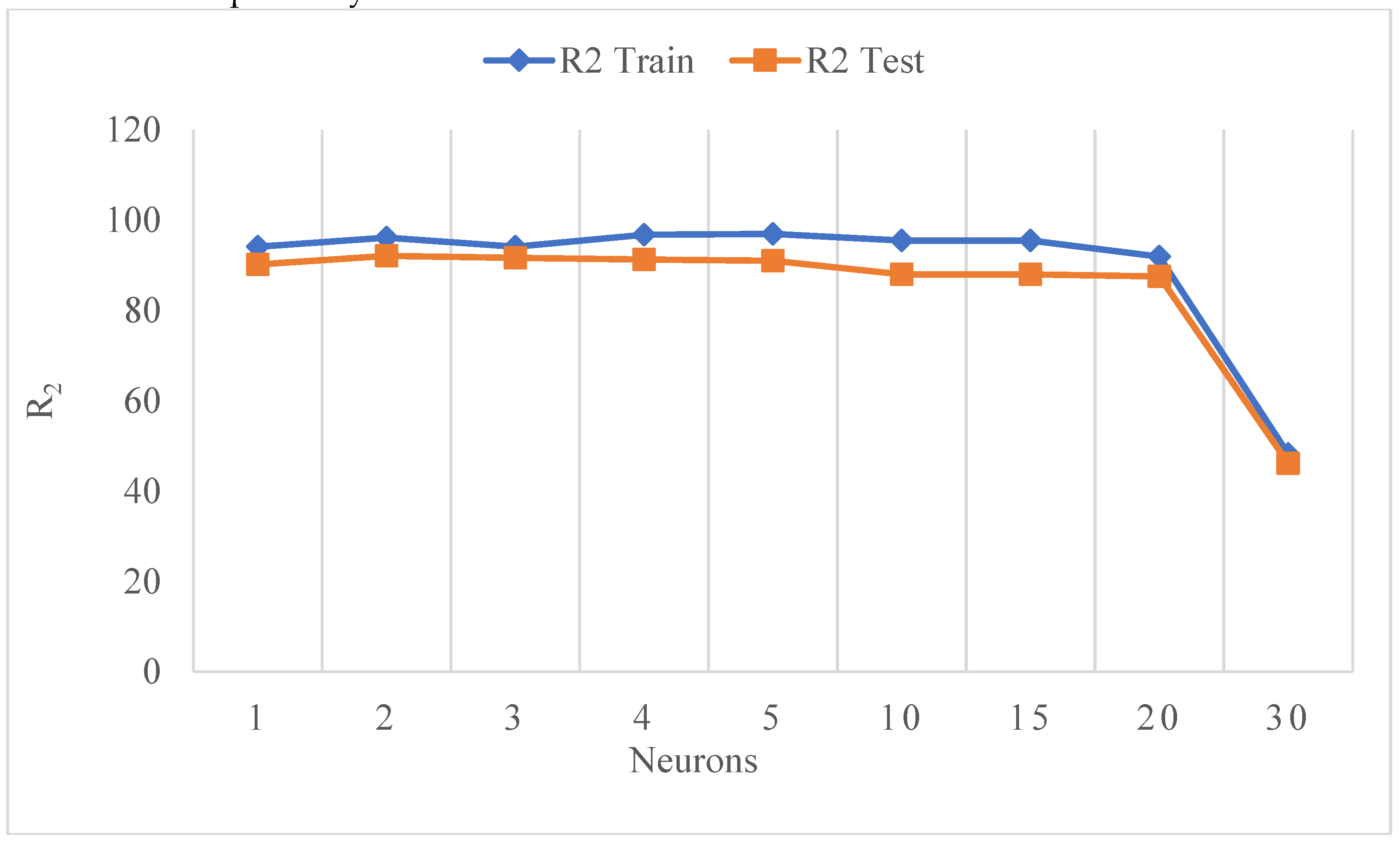
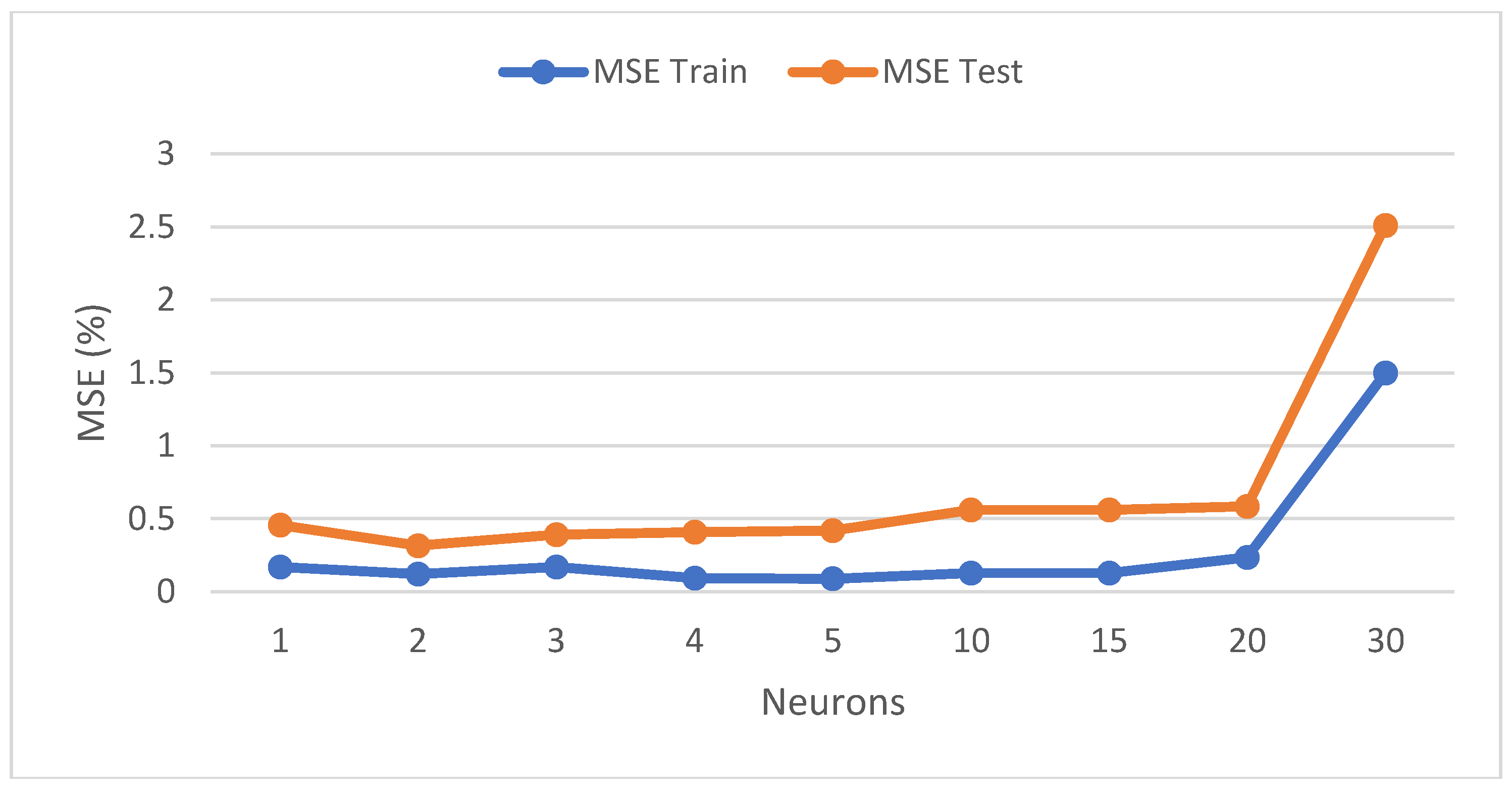
After executing the above parameters in Python, simulated outputs have been compiled and the accuracy of the model has been determined by calculating Mean Squared Error (MSE), Mean Absolute Error (MAE), and coefficient of determination (R2) through Python functions. MLP Regressor ANN mapping set of input data to output, the basis for this transformation is the number of nodes and number of hidden layers. Therefore, numerous models were developed by varying the number of hidden nodes and hidden layers, the performance results of the numerous models are summarized as shown in Table 7 and in Figure 4 and Figure 5. The best model was selected on the basis of model performance for the test datasets.

The results in Table 7 were obtained by selecting the maximum score the developed models show from two hundred different pieces of training for each in different number of nodes. Therefore, it is seen that the model with 2 hidden nodes can predict CLP with less MAE, and MSE values of 0.03060, and 0.00316 respectively. The R2 value for training datasets was 0.9611, demonstrating that the outputs/predictions are 96% close to the target values. Whereas the R2 value for the test dataset was 0.92065, which proves that the model is able to predict 92% of future outcomes accurately. Therefore, for the building construction projects located in Addis Ababa city, the MLP neural network structure with two hidden nodes shows maximum convergence and least error.

Figure 4 and Figure 5 display the effects of a number of neurons on the values of R2 and MSE respectively. R2 values range from 96% to 48% for train data sets and it ranges from 87% to 46% for test datasets. Whereas MSE values range from 0.094% to 1.497% for train data sets and it ranges from 0.316% to 2.511% for test datasets. Therefore, after comparing the results of R2 and MSE for the test datasets the model with one hidden layer and two hidden neurons shows maximum accuracy and least errors respectively.

Since the developed model will be used for future CLP rate estimation, the model with a high value of R2 with list error is selected as the optimal model to predict future concreting activity rates. It is observed during the model training phase that as the number of hidden layers increases the performance of a model will not be improved. Therefore, the model with two hidden neurons has a maximum accuracy and least error as compared to other models.

ANN is a sophisticated method that can predict CLP for building projects in Addis Ababa city with an average accuracy percentage of 92%. This average accuracy percentage was checked by using the 20% data that was left aside for this purpose. The data used for testing the performance of the model was not introduced during the training of the model, this separate data set for training and testing is important to accurately evaluate the performance of the developed model.

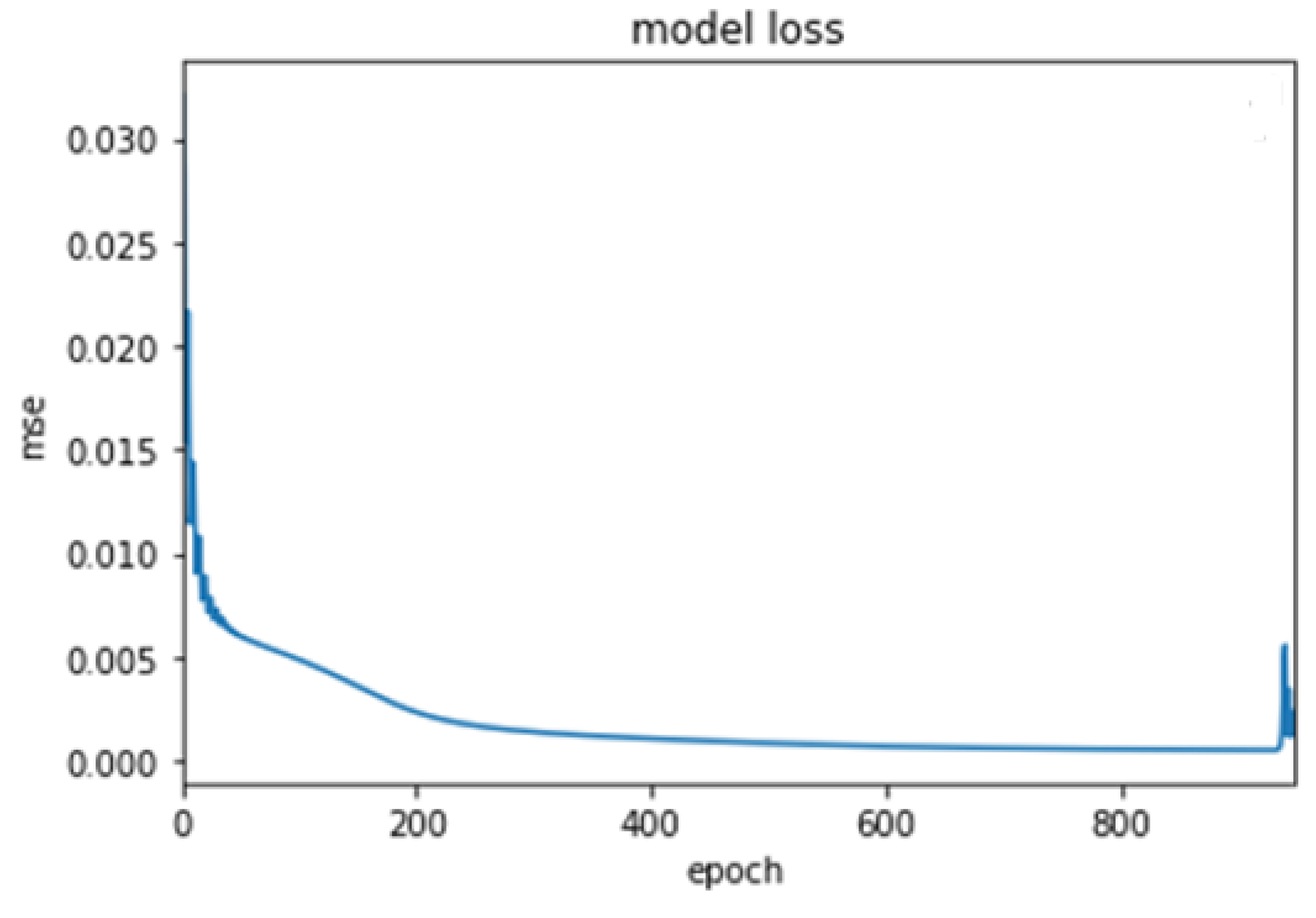
The minimum error observed for the optimal model was obtained after performing numerous trials and errors by varying the number of neurons in the hidden layer and the number of forwarding and backward iterations or epochs. Therefore, the minimum error was achieved with two hidden neurons and 1000 epochs as shown in Figure 6.

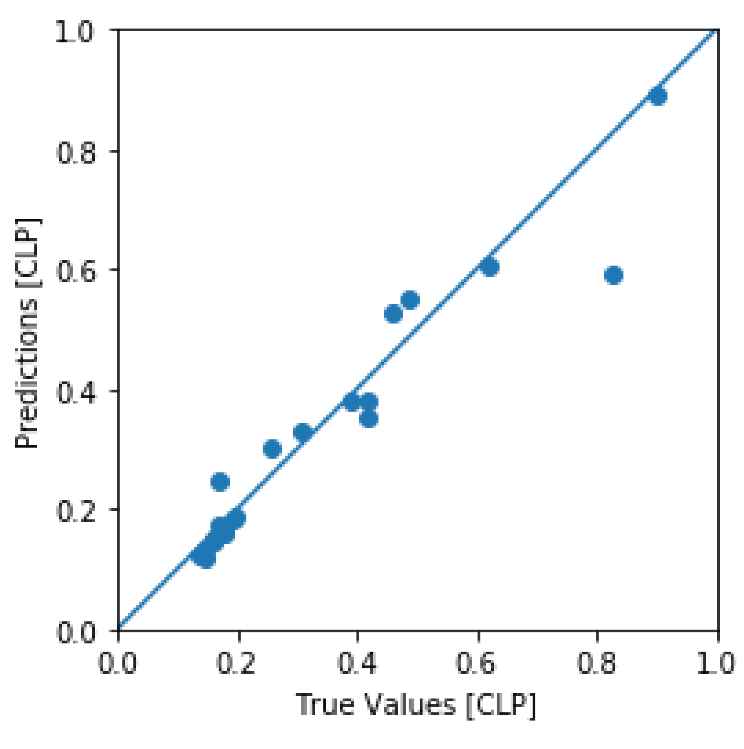
The scatter plot in Figure 7 shows the true and predicted values of productivity for the test dataset of 23 data samples that were selected and set aside for this purpose. The figure shows a good agreement between predicted and actual productivity values drawn in a 45-degree line. From the graph, we can conclude that the predicted productivity/machine guess values of productivity are approximately similar to actual values of productivity and the points observed around the 45-degree line shows a reasonable concentration of the predicted values of productivity. Therefore, the developed ANN model has a higher capability to predicting CLP of concreting activity.

3.5.2. Equation of the ANN model

The equation of ANN gives the value of an output node as a function of the values at the input nodes, bias, and connection weights. The connection weights and biases which are used for the final modeling are obtained from the optimal ANN models. The result of weights and biases for the optimal model is summarized in Table 8. Therefore, the coefficients and intercepts can be translated into formulas or mathematical models.

The CLP of concreting activity can be mathematically expressed using the connection weights and biases for the optimal model which are listed in Table 8 as follows:

X_{1} = [X_{1} \times W_{11} + X_{2} \times W_{12} + X_{3} \times W_{13} + X_{4} \times W_{14} + X_{5} \times W_{15} + X_{6} \times W_{16} + X_{7} \times W_{17} + X_{8} \times W_{18} + X_{9} \times W_{19} + X_{10} \times W_{110} + X_{11} \times W_{111} + {B H}_{1}]

(4)

X_{2} = [X_{1} \times W_{21} + X_{2} \times W_{22} + X_{3} \times W_{23} + X_{4} \times W_{24} + X_{5} \times W_{25} + X_{6} \times W_{26} + X_{7} \times W_{27} + X_{8} \times W_{28} + X_{9} \times W_{29} + X_{10} \times W_{210} + X_{11} \times W_{211} + {B H}_{2}]

(5)

But it should be noted that before adopting Equations 1 and 2 for estimation of CLP rates all the input values should be scaled between 0.1 to 0.9 ranges using min-max scaler formulas.

Then the values of X₁ and X₂ should be pass through sigmoid activation function as shown in Equation 6 and 7 bellow. If the values of X₁ and X₂ fails to pass through the sigmoid functions the non-linear relationship between the input and output variables can’t be established and the model performance can be affected. It is also a standard practice in ANN modeling to pass the values of X₁ and X₂ through the activation function.

X 1 H = \frac{1}{1 + e^{- x_{1}}}

(6)

X 2 H = \frac{1}{1 + e^{- x_{2}}}

(7)

Next the values of X₁H and X₂H should be multiplied with the corresponding weights based on Equation 5:

O = X_{1} H \times W_{11} H O + X_{2} H \times W_{12} H O + {B O}_{1}

(8)

Finally, the value of O which represents the scaled value of output should be converted into the unscaled predicted value of output using the min-max scaler formula.

To avoid the manual computation of CLP rate using this long formula and to avoid estimation mistakes the researcher built the required equation model using Excel programmed sheet. To apply and predict CLP for concreting activity only input data is required, so that the programmed Excel sheet automatically predicts the CLP rate.

Figure 8. Architecture of optimal model.

From Figure 8 it is clearly shown that the optimal model architecture has 11 input nodes, 2 hidden nodes, and 1 output node (11-2-1 node structure). This optimal model is a multilayer structure because it consists of three layers: input, hidden, and output layers. The optimal model was developed after 1000 times of forwarding and backward paths. During the forward path the network arbitrarily assigns numerical values to the weights and biases based on the data’s feed to the network, then the network compares the predicted values with actual values to calculate the error. Taking this error, the network propagates backward to adjust these weights and biases so that after 1000 iterations the model generates optimal values for weights and biases which can represent the data that was fed to the network. From the developed models the optimal model was the model with the least mean squared error and a high coefficient of determination value which was obtained after numerous trials and errors.

4. Discussion

The input parameters used in this model was previously investigated by many authors [1,12,29,30,31]. However, some of the parameters are site specific. The final optimal model has eleven variables in the input layer, one hidden layer with two nodes, and one node in the output layer which shows the optimal structure of the productivity of concreting activity in Addis Ababa city. This structure was practically enough for developing an optimal model using some sort of neural network parameters. To ensure the accuracy of the model and enhances model performance collected data have been systematically divided into training, validation, and testing dataset, with 65%, 15%, and 20% proportions respectively.

The average accuracy of the developed model is around 92%. A similar CLP model developed by [32] based on neural network for concrete pouring, had a accuracy value of 71%. Another CLP model developed by [7] based on fuzzy inference system also agree with the model developed in this research.

5. Conclusions

The productivity rate, which has a relationship with various factors, is one of the major components in determining the success or failure of a construction project. This paper attempts to show how to use AI models to predict labor productivity.

ANN model was developed based on the 114 datasets which were collected from Addis Ababa building projects. The developed model has the ability to predict the CLP rate of concreting activity with 92% of the coefficient of determination and 0.316% of MSE for the testing data set. This result shows that the developed model has a higher capability to predict CLP with an acceptable range of errors.

Construction stakeholders can easily use the programmed Excel sheet to predict the CLP of concreting activity for their future projects. Therefore, developing a construction labor productivity estimation model using ANNs for concreting activity, which was the general objective of this study is successfully achieved.

Author Contributions

Conceptualization, D.B.A and A.M.L; methodology, D.B.A and A.M.L.; software, D.B.A. and A.M.L; formal analysis, D.B.A and A.M.L.; investigation, D.B.A and A.M.L.; resources, D.B.A and Y.T.B.; data curation, D.B.A.; writing—original draft preparation, D.B.A and A.M.L.; writing—review and editing, A.M.L., Y.T.B, L.B; visualization, Y.T.B, L.B.; supervision, A.M.L. and L.B. All authors have read and agreed to the published version of the manuscript.

Funding

This research received no external funding

Institutional Review Board Statement

Not applicable

Informed Consent Statement

Not applicable.

Data Availability Statement

Not applicable.

Conflicts of Interest

The authors declare no conflict of interest.

References

Golnaraghi, S.; Zangenehmadar, Z.; Moselhi, O.; Alkass, S. Application of Artificial Neural Network (s) in Predicting Formwork Labour Productivity. Adv. Civ. Eng. 2019, 2019, 1–11. [Google Scholar] [CrossRef]
Muqeem, S.; Khamidi, M.F.; Idrus, A.; Zakaria, S. Bin Development of Construction Labor Productivity Estimation Model Using Artificial Neural Network. In Proceedings of the 2011 National Postgraduate Conference; IEEE; 2011; pp. 1–6. [Google Scholar]
Johari, S.; Jha, K.N. Impact of Work Motivation on Construction Labor Productivity. J. Manag. Eng. 2020, 36, 4020052. [Google Scholar] [CrossRef]
Girma, S.; Chimdi, J.; Mosisa, A. CHALLENGES OF USING PREFABRICATION TECHNOLOGY IN OROMIA REGIONAL STATE. J. Civ. Eng. Sci. Technol. 2020, 11, 22–27. [Google Scholar] [CrossRef]
Zenebe, E.; Quezon, E.T.; Mosisa, A. Contract Claim Analysis on Building Construction Project in Addis Ababa: A Case Study at Yeka Sub City. Int. J. Sci. Eng. Res 2016, 7, 1154–1160. [Google Scholar]
Sheikh, N.A.; Ullah, F.; Ayub, B.; Thaheem, M.J. Labor Productivity Assessment Using Activity Analysis on Semi High-Rise Building Projects in Pakistan. Eng. J. 2017, 21, 273–286. [Google Scholar] [CrossRef]
Assefa Tsehayae, A.; Robinson Fayek, A. Developing and Optimizing Context-Specific Fuzzy Inference System-Based Construction Labor Productivity Models. J. Constr. Eng. Manag. 2016, 142, 4016017. [Google Scholar] [CrossRef]
Khan, Z.U. Modeling and Parameter Ranking of Construction Labor Productivity, Concordia University, 2005.
Chimdi, J.; Girma, S.; Mosisa, A.; Mitiku, D. ASSESSMENT OF FACTORS AFFECTING ACCURACY OF COST ESTIMATION IN PUBLIC BUILDING CONSTRUCTION PROJECTS IN WESTERN OROMIA REGION, ETHIOPIA. J. Civ. Eng. Sci. Technol. 2020, 11, 111–124. [Google Scholar] [CrossRef]
Mekonen, H.; Legesse, A.M.; Ameya, F.M. Investigation of Price Escalation and Its Mitigation Mechanisms on Selected Building Construction Projects of Jimma University. Jordan J. Civ. Eng. 2023, 17, 194–202. [Google Scholar] [CrossRef]
Harmon, K.M.; Cole, B. Loss of Productivity Studies–Current Uses and Misuses. Constr. Briefings 2006, 8, 1–19. [Google Scholar]
Tsehayae, A.A. Developing and Optimizing Context-Specific and Universal Construction Labour Productivity Models, University of Alberta, 2015.
Tsehayae, A.A.; Robinson Fayek, A. Identification and Comparative Analysis of Key Parameters Influencing Construction Labour Productivity in Building and Industrial Projects. Can. J. Civ. Eng. 2014, 41, 878–891. [Google Scholar] [CrossRef]
Sarihi, M.; Shahhosseini, V.; Banki, M.T. Development and Comparative Analysis of the Fuzzy Inference System-Based Construction Labor Productivity Models. Int. J. Constr. Manag. 2021, 1–18. [Google Scholar] [CrossRef]
Yi, W.; Chan, A.P.C. Critical Review of Labor Productivity Research in Construction Journals. J. Manag. Eng. 2014, 30, 214–225. [Google Scholar] [CrossRef]
Elfaki, A.O.; Alatawi, S.; Abushandi, E. Using Intelligent Techniques in Construction Project Cost Estimation: 10-Year Survey. Adv. Civ. Eng. 2014, 2014, 1–11. [Google Scholar] [CrossRef]
Oduba, A.O. Predicting Industrial Construction Productivity Using Fuzzy Expert Systems, University of Alberta, 2002.
Gurmu, A.T.; Ongkowijoyo, C.S. Stochastic-Based Model for Setting Formwork-Productivity Baseline. J. Constr. Eng. Manag. 2020, 146, 4020099. [Google Scholar] [CrossRef]
Mohammadfam, I.; Soltanzadeh, A.; Moghimbeigi, A.; Savareh, B.A. Use of Artificial Neural Networks (ANNs) for the Analysis and Modeling of Factors That Affect Occupational Injuries in Large Construction Industries. Electron. physician 2015, 7, 1515–1522. [Google Scholar] [CrossRef] [PubMed]
Wang, Y.-R.; Gibson Jr, G.E. A Study of Preproject Planning and Project Success Using ANNs and Regression Models. Autom. Constr. 2010, 19, 341–346. [Google Scholar] [CrossRef]
Tam, C.M.; Tong, T.K.L. GA-ANN Model for Optimizing the Locations of Tower Crane and Supply Points for High-Rise Public Housing Construction. Constr. Manag. Econ. 2003, 21, 257–266. [Google Scholar] [CrossRef]
Yousefi, S.; Hegazy, T.; Capuruço, R.A.; Attalla, M. System of Multiple ANNs for Online Planning of Numerous Building Improvements. J. Constr. Eng. Manag. 2008, 134, 342–351. [Google Scholar] [CrossRef]
Heravi, G.; Eslamdoost, E. Applying Artificial Neural Networks for Measuring and Predicting Construction-Labor Productivity. J. Constr. Eng. Manag. 2015, 141, 1–11. [Google Scholar] [CrossRef]
Nasirzadeh, F.; Kabir, H.M.D.; Akbari, M.; Khosravi, A.; Nahavandi, S.; Carmichael, D.G. ANN-Based Prediction Intervals to Forecast Labour Productivity. Eng. Constr. Archit. Manag. 2020, 27, 2335–2351. [Google Scholar] [CrossRef]
Goodarzizad, P.; Mohammadi Golafshani, E.; Arashpour, M. Predicting the Construction Labour Productivity Using Artificial Neural Network and Grasshopper Optimisation Algorithm. Int. J. Constr. Manag. 2021, 1–17. [Google Scholar] [CrossRef]
Negnevitsky, M. Artificial Intelligence: A Guide to Intelligent Systems; Second.; Pearson education, 2005; ISBN 0321204662.
Haykin, S. Neural Networks: A Comprehensive Foundation Prentice-Hall Upper Saddle River; 2nd ed. 1999. [Google Scholar]
Beale, M.H.; Hagan, M.T.; Demuth, H.B. Neural Network Toolbox. User’s Guid. MathWorks 2010, 2, 77–81. [Google Scholar]
Aswed, G.K. Productivity Estimation Model for Bracklayer in Construction Projects Using Neural Network. Al-Qadisiyah J. Eng. Sci. 2016, 9, 183–199. [Google Scholar]
Al-Zwainy, F.M.S.; Abdulmajeed, M.H.; Aljumaily, H.S.M. Using Multivariable Linear Regression Technique for Modeling Productivity Construction in Iraq. 2013, 3, 128–135. [CrossRef]
Idrus, A.; Muqeem, S.; Khamidi, M.F.; Zakariya, M.S. Bin Estimating Construction Labor Productivity for Concreting Activity Using Artificial Neural Network. In Proceedings of the International Conference on Computer and Computational Intelligence; American Society of Mechanical Engineers; 2011; pp. 507–511. [Google Scholar]
Sonmez, R.; Rowings, J.E. Construction Labor Productivity Modeling with Neural Networks. J. Constr. Eng. Manag. 1998, 124, 498–504. [Google Scholar] [CrossRef]

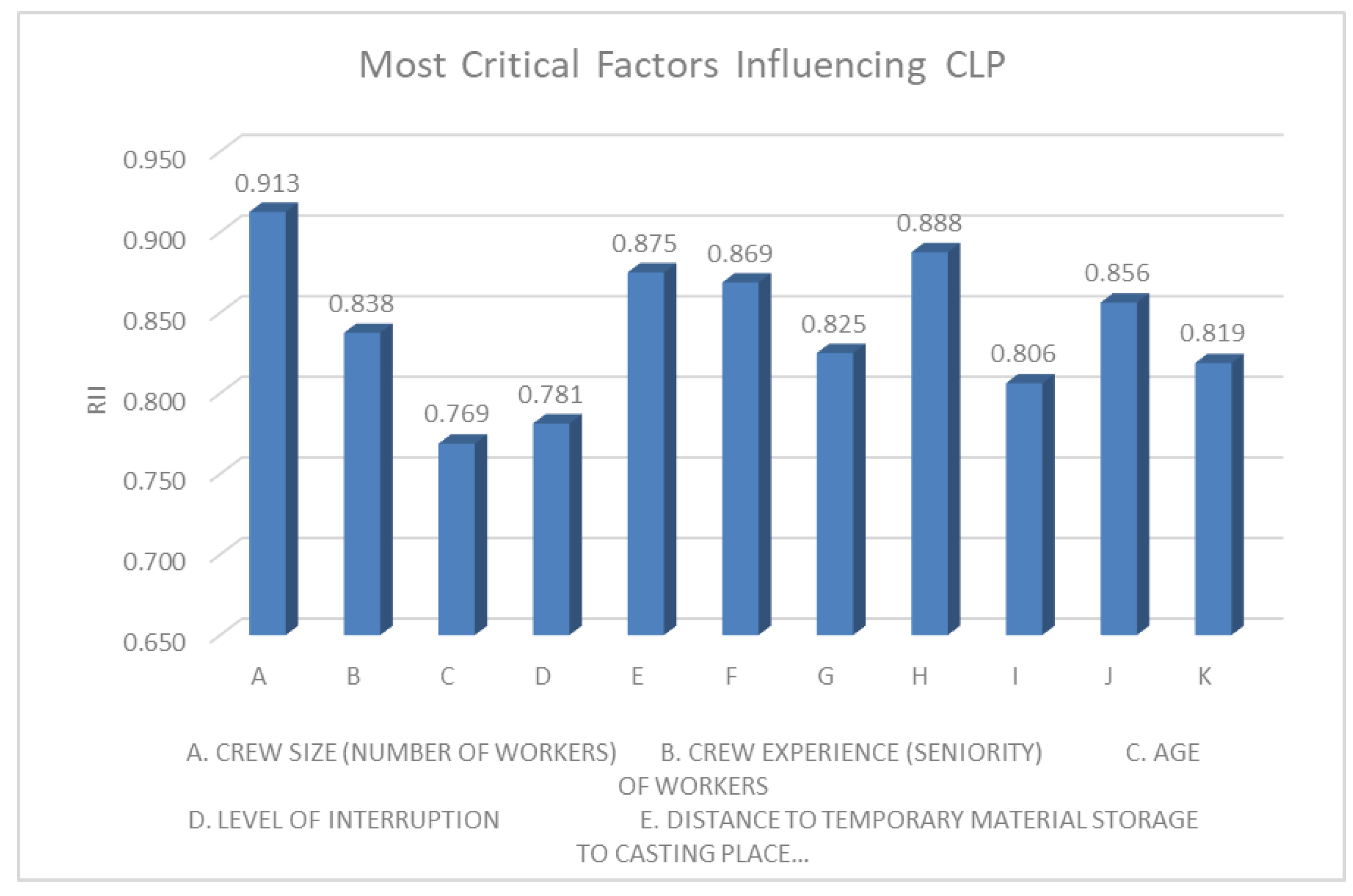
Figure 1. Most Critical Factors Influencing CLP.

Figure 2. Criteria for Selecting Building Projects for Data Collection.

Figure 3. Correlation Heat Map.

Figure 4. R2 Values with their Corresponding Neurons.

Figure 5. MSE of Different Models with their Corresponding Neurons.

Figure 6. Training Mean Squared Error.

Figure 7. Scattered Plot of Predicted and Actual Rates.

Table 1. quantitative and qualitative labor productivity factors.

S.No.	Objective (Quantitative) factors	Subjective (Qualitative) factors
1	Crew Size (number of workers)	Weather condition (comfort level)
2	Crew experience (seniority)	Location of project
3	Age of workers	Comfortability of materials storage for work
4	Average wind speed	Scaffold requirement
5	Number of consecutive days worked	Skill level of labor
6	Number of languages spoken	Congested work area (arrangement of falsework)
7	Number of craftsperson technical training	Communication problems with workers
8	Level of overtime	Alcoholism
9	Level of interruption and disruption	Disruption of power/water supplies
10	Foreman experience	Health status of workers
11	Distance to temporary material storage to casting place	Extent and quality of supervision
12	Space of casting (volume of work)	Safety requirements
13		quality requirements
14		Crew flexibility (crew willingness in performing other members task)
15		Building element (footing, grade beam, column, slab…)
16		Cover from weather effect
17		The working condition (noise)
18		Placement technique (Pump, Crane, bucket, direct chute…)

Table 3. Summary of the Collected Data Set.

Table 4. Correlation between CLP and Influencing Factors.

Influencing Factors	Correlation(R)
Crew Size	0.1160
Crew Experience	0.5681
Age	0.5349
Interruption level	-0.0573
Distance	-0.1201
Whether	-0.0748
Congested Area	-0.1944
Health Status	-0.1984
Crew Flexibility	-0.0912
Building Element	0.1266
Placement Techniques	-0.5227

Table 5. Optimal Model Data Division.

Type of Dataset	Number of Data Instances	Percentage (%)
Training	74	65
Validation	17	15
Testing	23	20
Total	144	100

Table 6. The Optimal ANN Model Parameters.

Document String Type	Description
Hidden layer size	Number of layers and neurons are introduced (1 hidden layer and 2 hidden nods)
Activation	Activation used in the hidden layer (Logistic)
Maximum iterations	Number of epoch (2000)
Solver (Optimizer)	For weight optimization (Adam)
Initial learning rate	Controls weights and bias update (0.1)
Momentum	For gradient decent update(0.9)
Early stopping	Stops training when loss stops decreasing (True)
Validation fraction	Set aside data for validation (15%)

Table 7. Performance Results of One Hidden Layer Model.

MAE Train		MSE Train		R² Train
Train	Test	Train	Test	Train	Test
0.03253	0.04141	0.00170	0.00457	0.94080	0.90182
0.02051	0.03060	0.00121	0.00316	0.96110	0.92065
0.02962	0.03561	0.00170	0.00391	0.94105	0.91596
0.02136	0.03395	0.00094	0.00407	0.96739	0.91253
0.02016	0.03621	0.00088	0.00420	0.96924	0.90972
0.02652	0.04498	0.00129	0.00562	0.95500	0.87939
0.02652	0.04498	0.00129	0.00562	0.95500	0.87939
0.03276	0.04400	0.00234	0.00583	0.91867	0.87482
0.08388	0.11183	0.01497	0.02511	0.48165	0.46114

Table 8. Optimal Model Weights and Biases.

Weights between input nodes and hidden node 1	Weights between input nodes and hidden node 2	Hidden Biases	Hidden to output weights	Output bias
W₁₁= -0.80771825	W₂₁= -1.29754431	BH₁ = 0.358 34581 BH₂ = -1.508 88807	W₁₁H_O= -0.6679519 W₁₂H_O= -1.62451474	B₀₁= 1.955 71816
W₁₂= 0.145702103	W₂₂= -2.42387211
W₁₃= -0.528524606	W₂₃= 2.26612486
W₁₄= 0.201301486	W₂₄= 2.74387717
W₁₅= 0.132271702	W₂₅= -0.026419671
W₁₆= 0.0334985595	W₂₆= -0.00353481671
W₁₇= -0.0949299372	W₂₇= 0.00908773745
W₁₈= -0.282357359	W₂₈= 0.336306823
W₁₉= 0.103049981	W₂₉= 0.588741942
W₁₁₀= -0.214612051	W₂₁₀= 2.39695108
W₁₁₁= -1.21460908	W₂₁₁= 10.5258561

Disclaimer/Publisher’s Note: The statements, opinions and data contained in all publications are solely those of the individual author(s) and contributor(s) and not of MDPI and/or the editor(s). MDPI and/or the editor(s) disclaim responsibility for any injury to people or property resulting from any ideas, methods, instructions or products referred to in the content.

© 2024 by the authors. Licensee MDPI, Basel, Switzerland. This article is an open access article distributed under the terms and conditions of the Creative Commons Attribution (CC BY) license (http://creativecommons.org/licenses/by/4.0/).

Copyright: This open access article is published under a Creative Commons CC BY 4.0 license, which permit the free download, distribution, and reuse, provided that the author and preprint are cited in any reuse.

MDPI Initiatives

Important Links

Choose an area of interest and we will send you notifications of new preprints at your preferred frequency.

Disclaimer

Developing Construction Labor Productivity Model for Concreting Activity Using Artificial Neural Networks

Abstract

1. Introduction

2. Materials and Methods

2.1. Model Development

2.2. Mathematical Steps for the Training Algorism into ANN’s

3. Results

3.1. Identification of input Parameters

3.2. Quantification of Input Parameters

3.3. Data Analysis

3.4. Optimal Data Division

3.5. ANN Optimal Parameters

3.5.1. Effects of Hidden Nodes on Performance of NN’s

3.5.2. Equation of the ANN model

4. Discussion

5. Conclusions

Author Contributions

Funding

Institutional Review Board Statement

Informed Consent Statement

Data Availability Statement

Conflicts of Interest

References

MDPI Initiatives

Important Links

Subscribe