Point Cloud Densification Algorithm for Multiple Cameras and Lidars Data Fusion

1. Introduction

The fused data allows a more accurate analysis due to the usage of a complete, multidimensional description of the world. Combining data from various sources became more and more popular, both due to the growing number of sensors and the increasing computing power of computers. Fusing multiple camera images with lidar point-clouds has applications in augmented reality, robotics and autonomous driving. This process increases the quality of object detection and object classification in terms of both sensitivity and specificity.

The camera produces two-dimensional (2D) images. It is a dense regular grid of pixels with a particular colour.

Due to progress in digital camera construction (using CCD or CMOS sensors), images contain a very large number of such pixels, for example, $1920\times 1080\approx 2$ million pixels. The typical colour depth is almost 24 bits = $\approx 16$ million.

Three-dimensional (3D) lidar scaner, on the other hand, produces point clouds in three-dimensional space. A point cloud consists of a number of points described by the three coordinates x, y and z representing the location of a point and possible attributes of that point, such as the intensity of light reflected by the object. Lidar point clouds do not contain information about the entire space and may have an irregular structure. Depending on the equipment used and the space being observed, point clouds points may contain a varying number of points, but this number is far smaller than the number of pixels in the images, typically around $100,000$ points. In addition, the point cloud becomes sparser as the distance from the sensor increases, so that an object far from the sensor may not be visible in the cloud.

The problem of fusing camera images with 3D lidar clound-points is important and widely discussed in the literature since such sensors were developed [1,2,3]. The fusion needs common coordinate system for all fused sensors. In the literature the three approaches are most popular[4]:

• point cloud densification – creation of point clouds based on pairs of stereovision images and camera calibration data, then combining point clounds;
• coloring of lidar point cloud based using colours from camera images;
• projection 3D lidar data on 2D, then fusing 2D images.

The most promising method is point cloud densification, i.e., adding to the existing lidar point cloud, new points obtained by reconstructing three-dimensional space [5]. It was applied in moving platforms (aircraft, boat, automobile) [6], and has many application in geodesy, cartography, environmental monitoring, object detection and others.

Combining several point clouds, e.g., from multiple lidars, is a fairly straightforward operation; it basically involves creating a new point cloud containing points from several clouds, remembering to first transform them to the same coordinate system by multiplying the matrix containing the points by an extrinsic calibration matrix describing rotation and translation.

Indeed, a more difficult problem is to obtain a point cloud from camera data. The problem becomes easier for a pair of stereoscopic images. Obtaining a point cloud from such a pair of images requires finding a pixel match between the images and calculating a disparity map.

Assuming a pinhole camera model and projective geometry (extension to Euclidean geometry where points of intersection of lines are considered), moreover, considering two cameras with the same focal length and placed in such a way that their planes are parallel we can show that the pixels corresponding to the same point in 3D are in the same row in both images, they have the same y coordinate value, [7].

Based on the disparity and camera parameters, the distance of the objects from the camera can be calculated, thus the coordinates of the 3D points. A projection matrix, which is a composite of the camera’s intrinsic matrix – describing its intrinsic parameters – and an extrinsic calibration matrix, the same as for lidar, for example, describing rotation and translation, is used to obtain points in the appropriate coordinate system. Pixels with calculated depth are multiplied by this matrix to get 3D points.

There are several methods used to solve pixel matching problem, for example based on absolute difference sum, or mutual correlation or global optimization of the cost function or dynamic programming[8]. Dynamic programming is often used to solve optimization problems. It involves dividing a complex problem into many smaller subproblems [9]. These subproblems are not independent of each other, but are solved sequentially. The key to designing a dynamic programming algorithm is to find a suitable recursive equation.

Matching pixels in a pair of images can be found with the Needleman-Wunsch algorithm [10]. This is an algorithm based on dynamic programming, originally used for amino-acid or nucleic-acid sequence alignment. In our work, we adapt it to the problem of finding matching pixels and then calculating the coordinates of three-dimensional points. Such technique was also mentioned in review [11].

There are open libraries and tools allowing the processing of camera and lidar data. The most popular are:

• Point Cloud Library (PCL) [12] - a popular library for point cloud processing, is a free and open-source solution. Its functionalities are focused on laser scanner data, although it also contains modules for processing stereo vision data. PCL is a C++ language library, although unofficial Python language bindings are also available on the web, e.g., [13], which allows you to use some of its functionality from within the Python language.
• OpenCV [14] - one of the most popular open libraries for processing and extracting data from images. It also includes algorithms for estimating the shapes of objects in two and three dimensions from images from one or multiple cameras and algorithms for determining the disparity map from stereovision images and 3D scene reconstruction. OpenCV is a C++ library with Python bindings.

We improved the dynamic programming algorithm performance by reducing the size of matched pixels determined by available car speeds, implementing it in C++ using parallel computing available on modern computer platforms. We developed a new library containing this algorithm, providing a solution that is fully and easily accessible from the Python language. In addition, we also cared about the best possible quality results, by using the affine gap penalty function and filling the not-matched pixels with the colours of their neighbours.

In the remainder of the paper, we discuss our fusion method in detail, particularly the proposed stereo-matching algorithm inspired by the algorithm used in bioinformatics and how to obtain the final disparity map based on the obtained matching. We describe the new methods used to improve the quality and the performance. In Section 3 we discuss the results of the proposed algorithm, present the benchmark datasets used and compare the results of our algorithm with others popular methods. Finally, in Section 4 and Section 5, we summarize information about the implemented library, discuss the possible applications and further research directions.

2. Materials and Methods

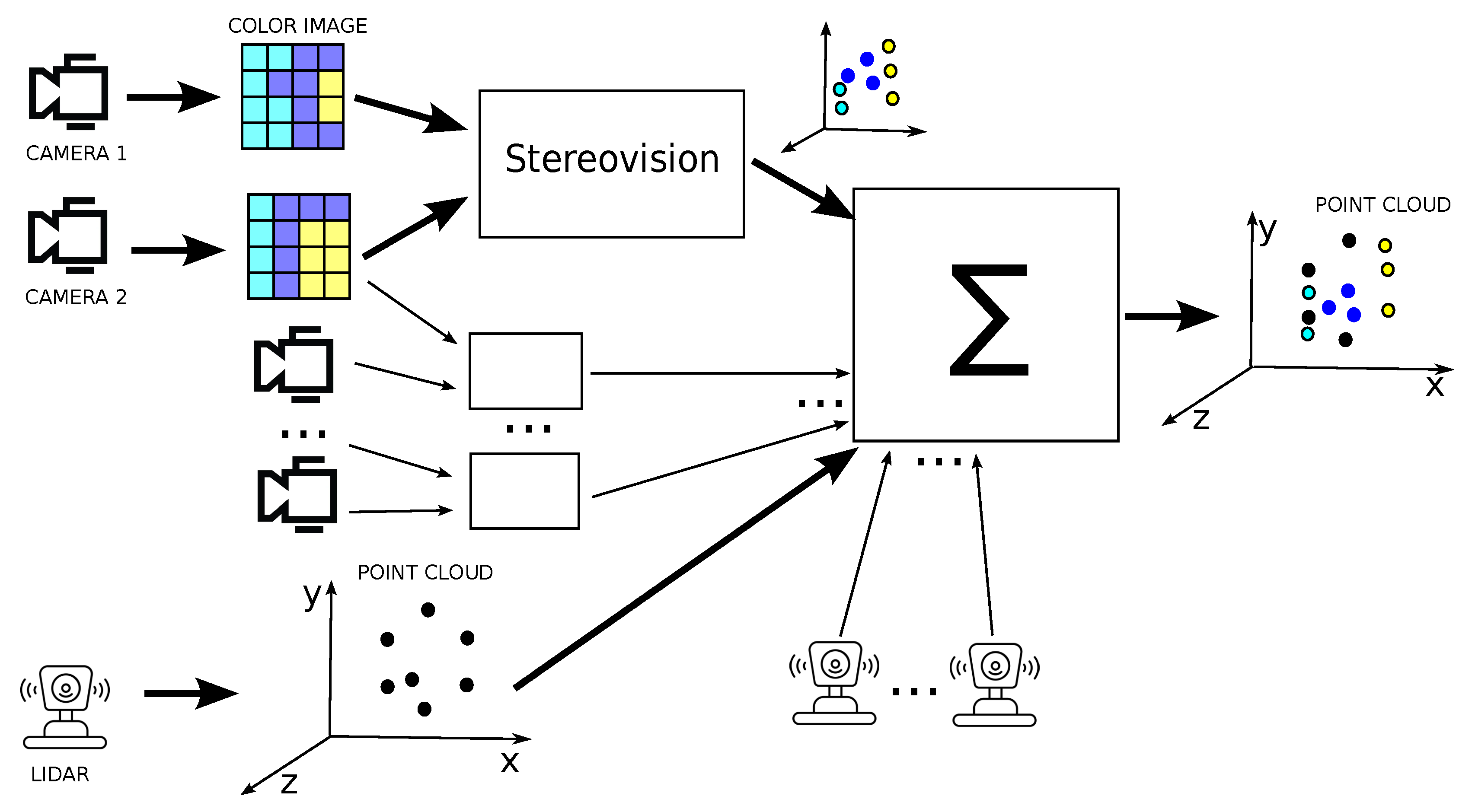
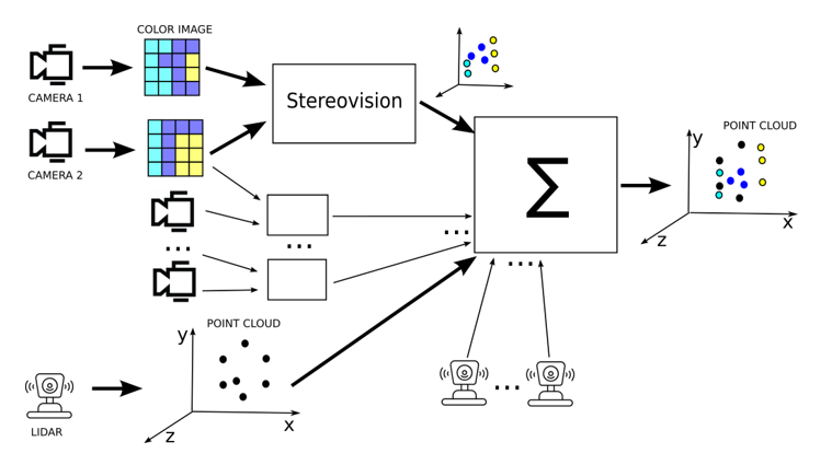
Presented approach is realisation of point cloud densification idea. New method form stereovision is proposed, then point clouds are combined by transformation to the same coordinate system, as depicted in Figure 1.

2.1. New Algorytm for Sterovision

Assuming a pinhole camera model, considering two cameras producing stereoscopic images, to matching image of pixels (2D array) we can properly match sequences of the pixels, because the pixels corresponding to the same point in 3D are in the same row in both images, they have the same y coordinate value [7].

When matching pixels on a pair of stereovision images, the idea is to find the best match, such as the best pixel match in each line of images. By using a dynamic programming algorithm, similar pixels can be matched and non-matching pixels can be skipped. For this purpose, we adapted the Needleman-Wunsch algorithm to the pixel sequence matching problem.

The need for pixel skipping is due to the fact that we want to match one pixel from one line with one pixel from the other line, and the fact that there are situations when a given fragment of space is visible only in one image, because at different camera positions different fragments of space are invisible, for example obscured by an object closer to the camera. In such a situation, the pixel representing the color of such a fragment of space should not be matched with any pixel from the other image. However, the problem of matching pixels requires the use of a different matching function and a different gap penalty function than in the original version of the algorithm - other than a constant.

In each step of the algorithm, the value of the recursive equation is calculated for the corresponding arguments by reading the previously calculated values from an auxiliary matrix, the cells of which are completed in subsequent steps of the algorithm.

A measure of the alignment of pixels is a measure of their similarity. In our solution, we used the sum of the absolute differences of the color channels in the color space as the similarity function. The color similarity function in RGB space is represented by the Equation (1), where $e(i,j)$ is the similarity of the i-th pixel from the left image with the j-th pixel from the right image, $e_{max}$ is the highest possible similarity (set as a parameter), $P\left(i\right)$ is the value of the pixel’s color channel, the letters in the subscripts denote the channel (R, G or B) and the image (left or right) from which the value is read.

$$e(i,j)=e_{max}-\left(\right|P_{R,l}\left(i\right)-P_{R,r}\left(j\right)|+|P_{G,l}\left(i\right)-P_{G,r}\left(j\right)|+|P_{B,l}\left(i\right)-P_{B,r}\left(j\right)\left|\right)$$

(1)

This function can take both positive values, meaning a lot of similarity, and negative values, meaning a lot of difference.

The algorithm does not require that the images be saved using a specific color space, it can be RGB, YUV or grayscale, for example. Because the Needleman-Wunsch algorithm assumes that the matching function returns positive values (indicating a match) and negative values (indicating no match) the parameter of our algorithm is the reward for a perfect match - a match of pixels with identical color. This is a value added to the calculated color difference. The values of penalties and rewards given as parameters of our algorithm should have an absolute value less than 1, in a further step they are scaled accordingly.

For each pair of pixels, the most beneficial action is calculated. The possible actions for a pair of pixels are to associate them with each other or to insert a gap (hole) on one line, i.e., to skip a pixel. The choice of action is influenced by the values in the neighboring cells of the auxiliary matrix, the alignment of the pixels and the cost of performing the gap. The cost of a gap in our solution is interval-constant (a different penalty for starting a gap and a different penalty for continuing a gap - omitting the next neighboring pixel on one of the lines). The penalty for the n-th pixel gap was defined by the Equation (2), where $d_{start}$, $d_{continue}$ are the parameters of the algorithm.

$$d\left(n\right)=\left\{\begin{array}{cc}{d}_{start}\hfill & n=0\hfill \\ d_{continue}\hfill & n=1\hfill \\ 0\hfill & n>1\hfill \end{array}\right.$$

(2)

The choice of such a gap penalty resulted from the observation that the points to which neighboring pixels correspond are close to each other - they belong to the same object, or far from each other - they are on other objects. If the points lie on a straight line parallel to the plane of the cameras, the difference between successive matched pixels is the same, if the line is not parallel, but the points belong to the same object, this difference should not vary significantly, and in the case where the points do not belong to the same object, the difference between neighboring matches is greater and depends on the distance between the objects.

The Equation (3) contains the definition of the recursive formula used in the stereovision-adapted version of the Needleman-Wunsch algorithm.

$$F(i,j)=max\left\{\begin{array}{c}F(i-1,j-1)+e(i,j)\hfill \\ F(i-1,j)+d\left(n\right)\hfill \\ F(i,j-1)+d\left(n\right)\hfill \end{array}\right.$$

(3)

In this formula, $F(i,j)$ denotes the value in the i-th row and j-th column of the auxiliary matrix, $e(i,j)$ is the pixel match - the reward (penalty) for the match, and $d\left(n\right)$ denotes the gap penalty function. The best match is obtained by finding the path from the last cell of the auxiliary matrix (from the bottom right corner) to its first cell (top left corner), always choosing the action whose value is the largest.

For example, if we match lines (sequence of pixels) shown on Figure 2, where we denote first line as $s=s_0{s}_1{s}_2{s}_3{s}_4{s}_5$, and second line as $t=t_0{t}_1{t}_2{t}_3{t}_4{t}_5$ (in the example we assume lines on image have 6 pixels), and we denote colours as A, B and C, therefore $s=AABCCC$, $t=ABBBBC$, and use the example values of similarity from Equation (1), , and the penalthy $d=-5$, the results is or matched pixels are $(s_0,t_0),(s_1,t_3),(s_2,t_4)$. The $F(i,j)$ from Equation (3), and results are depicted in Figure 2.

Figure 2 shows, the auxiliary matrix of the algorithm with the matches and gaps marked. The gaps have an additional indication of which image they are visible in.

Matching sequences with the Needleman-Wunsch algorithm requires filling the auxiliary matrix, that is, completing all its $N^2$ cells, and finding a path from the lower left to the upper right corner of the matrix, which requires N operations. The computational complexity of the algorithm is thus $O\left(N^2\right)$.

2.1.1. Disparity Map Calculation Based on Matching

Adaptation to the problem of finding matching pixels on a pair of images also required the second step of the algorithm. In our implementation, when finding the best path in the filled auxiliary matrix, a disparity map (an image containing the distances between images of the same point on the plane of the two cameras) is completed based on the coordinates of the cells corresponding to the matched pixels. For each match, a value of $x_r-x_l$ or $x_l-x_r$ is stored in the disparity map, where $x_l$ and $x_r$ are the coordinates of the matched pixels in the left and right images.

The disparity map calculated in this way contains only the values for those pixels for which matching has happened. To obtain a complete disparity map, it is necessary to fill in the holes that appear. We mentioned in the Section 2.1 that the gaps are due to the fact that a given section of space is visible from only one camera.

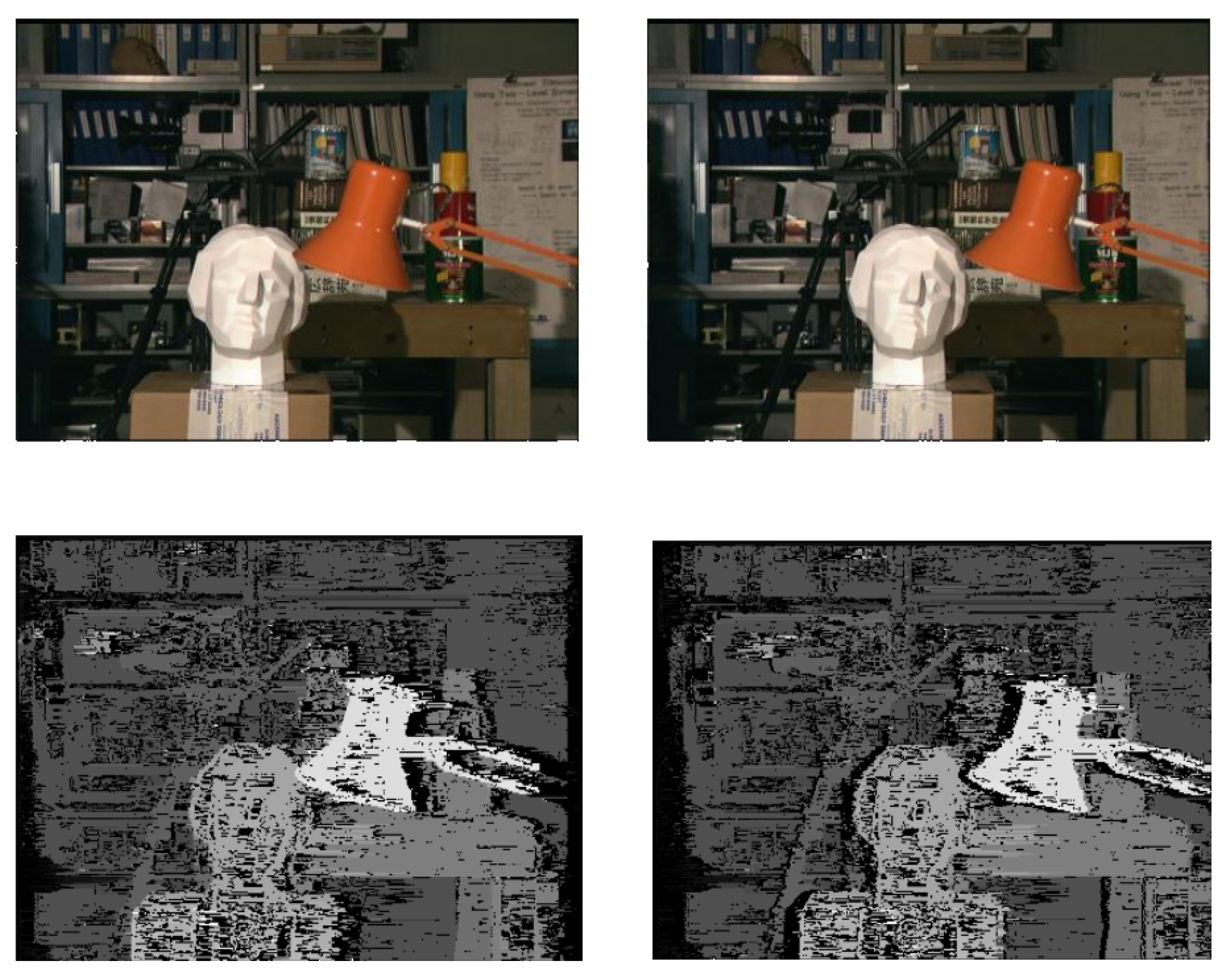
The Figure 3 shows a series of images with marked gaps relative to the center (reference) image, and the Figure 5 shows the holes computed using the algorithm from our Stereo PCD library without hole filling.

For this reason we fill in the holes based on the value of the pixel neighboring the gap, corresponding to the portion of space further away from the camera plane.

2.1.2. Improving the Quality of Matching through Edge Detection

The first enhancement we propose is due to the desire to use additional information, aside from color, on which to compare pixels. The enhancement we propose uses the Harris feature and edge detector [16]. It is a fast corner and edge detector based on a local autocorrelation function. It works with good quality on natural images.

In our solution, we use the information, about edges, to add an additional reward for matching if both related pixels are on an edge.

Another rather simple but, as it turned out, effective improvement relates to the filling of gaps in disparity maps. We propose to use both neighbors of the gap and information about any pixels recognized as edges and inside the hole to fill the gap. The value of the neighbor previously unused in filling the hole is now used to fill it up to the first pixel recognized as an edge, while the rest of the hole is filled as before by the other neighbor.

2.1.3. Performance Improvement Reducing Length of Matched Sequences

We have also applied improvements to produce a result in less time. The first improvement takes advantage of the fact that it is not necessary to compare all pixels from a given line from one image with all pixels from the corresponding line from the other image. This is because, knowing the parameters of the measurement set, it is possible to determine at what minimum distance the object is from the camera and, therefore, to determine the maximum value of the disparity. In addition, knowing which image contains the view from the left and which from the right camera, allows you to consider that the minimum disparity is 0. The use of these two facts allows you to reduce the number of pixels compared with each other. Most often, a single pixel from a single image only needs to be compared with several times fewer pixels than when whole lines are compared. Thus, the application of this improvement improves the computational complexity of the pixel-matching algorithm on a pair of images. The original complexity is $O\left(H{W}^2\right)$, where H is the height of the image and W is the width of the image - this is due to the need to fill a square matrix with $W^2$ cells for each H line. Using the disparity constraint reduces the computational complexity to $O\left(HWD\right)$, where D is the maximum value of the disparity (smaller than the image width W). 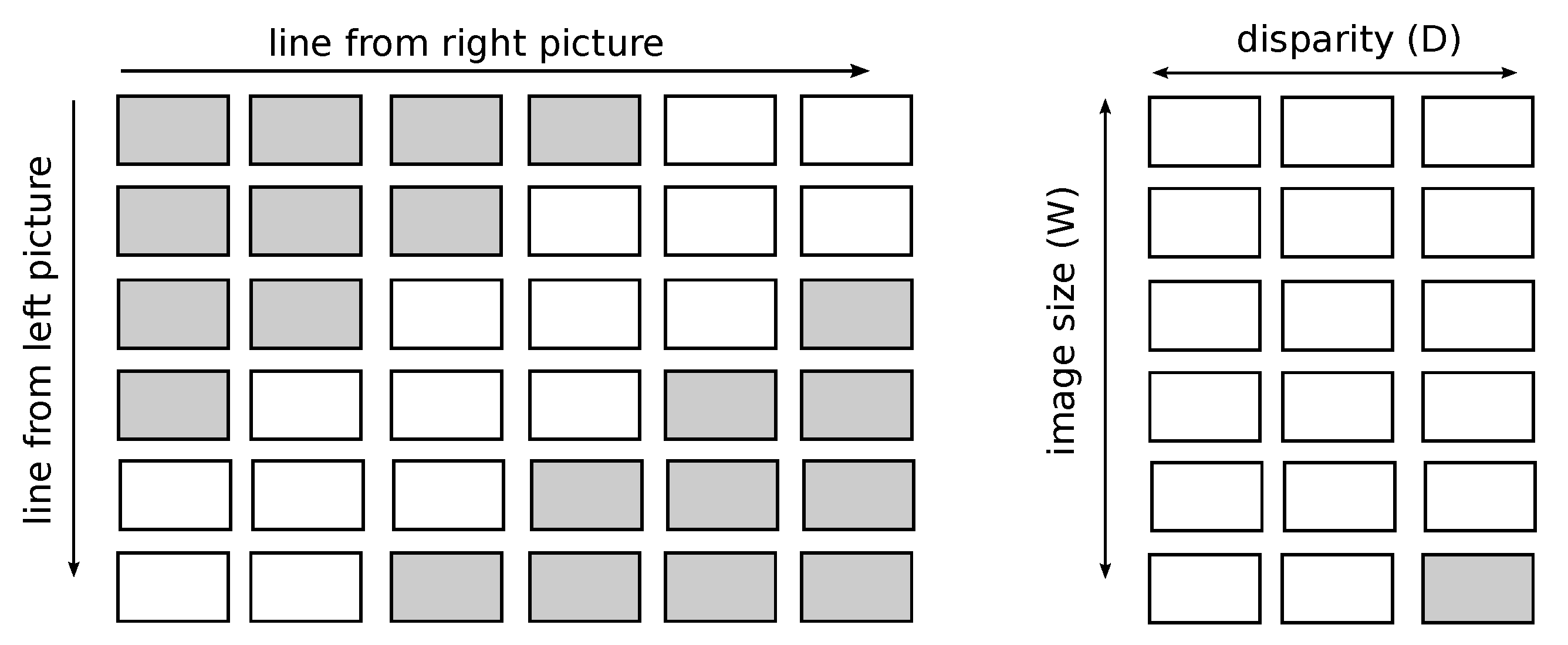The improvement is due to the need to fill in at most D (instead of W) cells in W rows of the auxiliary matrix. Moreover, taking advantage of this fact, we decided to write this array in such a way that it takes up less memory. Instead of allocating an array of size $W\times W$, we only need an array of size $W\times D$, so that the number of columns is equal to the maximum number of comparisons for a single pixel. Applying such a trick, however, required changing the indexes of the cells used to calculate the value to be written in the next cell of the array - the indexes of the cells read from the row above the complement increased by 1. This is shown in Figure 4.

2.1.4. Parallel Algorithm for 2D Images Matching

The next improvement takes advantage of the fact that lines (rows of pixels) are matched independently of each other. This allows you to analyze several lines in parallel. For this purpose, we use multithreading in our solution. Each thread allocates its buffers for data, e.g., the auxiliary matrix used in the algorithm, and then takes the value of the line counter and increments its value. Synchronization is ensured so that two threads do not fetch the same line number. The thread then matches the pixels on that line, fetches the next line number, matches the pixels on that line, and the process repeats until the calculations for all lines are done.

Figure 5. Images from the ’head and lamp’ dataset [17] along with the determined disparity map for the left and right images without filling in the gaps.

Figure 5. Images from the ’head and lamp’ dataset [17] along with the determined disparity map for the left and right images without filling in the gaps.

3. Results

The algorithm presented in our work has been implemented in C++ and placed in the Stereo PCD open library, along with other tools supporting the process of combining camera and lidar data. The library is accessible from the Python language level, and the algorithm implemented in C++ was placed in it thanks to the binding. The algorithm from the Stereo PCD library was tested on publicly available and frequently used for evaluating the quality of stereovision algorithms datasets.

3.1. Datasets

To evaluate the quality and performance of the algorithm used to find pixel matches on a pair of stereovision images, we used open and online datasets. The number of algorithm rankings on the [18] and [19] indicates the popularity of the selected datasets.

3.1.1. University of Tsukuba ’Head and Lamp’

The ’head and lamp’ dataset [17] consists of images showing a view of the same scene showing, among other things, a head statue and a lamp. The dataset is made up of low-resolution images, which allows the disparity to be calculated fairly quickly even with a low-performance algorithm, which is very useful in the development and initial testing stages. The dataset is available at [18].

Figure 6. Examples of images from the ’head and lamp’ dataset with a reference disparity map.

Figure 6. Examples of images from the ’head and lamp’ dataset with a reference disparity map.

3.1.2. Middlebury 2021 Mobile Datasets

The Middlebury 2021 mobile datasets [18,20] was created by Guanghan Pan, Tiansheng Sun, Toby Weed and Daniel Scharstein in 2019-2021. The dataset contains high-resolution images that were taken indoors using a smartphone mounted on a robotic arm. The dataset is available at [18].

Figure 7. A pair `artroom1’ images from the Middlebury 2021 mobile dataset, along with a reference disparity map.

Figure 7. A pair `artroom1’ images from the Middlebury 2021 mobile dataset, along with a reference disparity map.

3.1.3. KITTI

The KITTI dataset [19,21] was developed by the Karlsruhe Institute of Technology and the Toyota Technological Institute at Chicago and published in 2012. The data was collected from sensors placed on the moving car including stereo cameras and lidar. Based on the data collected over 6 hours of driving, datasets were created to test algorithms including object detection and tracking and depth estimation based on image pairs. The datasets are available at [19].

Figure 8. Examples of images from the KITTI dataset with a reference disparity map.

Figure 8. Examples of images from the KITTI dataset with a reference disparity map.

3.2. Quality Evaluation Method

In order to evaluate the effects of matching and to select the parameters of the algorithm, it is necessary to be able to estimate the quality of the matching, and to be able to assess which matching is better. A typical approach to this type of issue is the calculation of error statistics. Such statistics are usually calculated by comparing the obtained result with a pattern from the provided dataset.

Quite popular metrics for this problem used in [15], among others, are the root of the mean square error defined by the Equation (4) and the percentage of correct matches calculated from the Equation (5),

$$RMSE=\sqrt{{\displaystyle \frac{1}{N}}{\sum }_{(x,y)}{(d_C(x,y)-d_G(x,y))}^2}$$

(4)

$$GPR={\displaystyle \frac{1}{N}}\sum _{(x,y)}\left(\right|d_C(x,y)-d_G(x,y)|<{\delta }_d)$$

(5)

where $d_C$ is the calculated disparity value for a given pixel, $d_G$ is the benchmark disparity value for a given pixel, N is the number of pixels evaluated, and ${\delta }_d$ is the acceptable matching error. If the error is less than ${\delta }_d$ then the pixel is considered to be correctly matched.

Since there are several ways to calculate quality metrics, we decided to implement a function to calculate such quality metrics in the Stereo PCD library. The library implements evaluation methods with skipping pixels without disparity values and considering pixels without values in the calculated disparity maps as bad matches.

3.3. Quality Tests

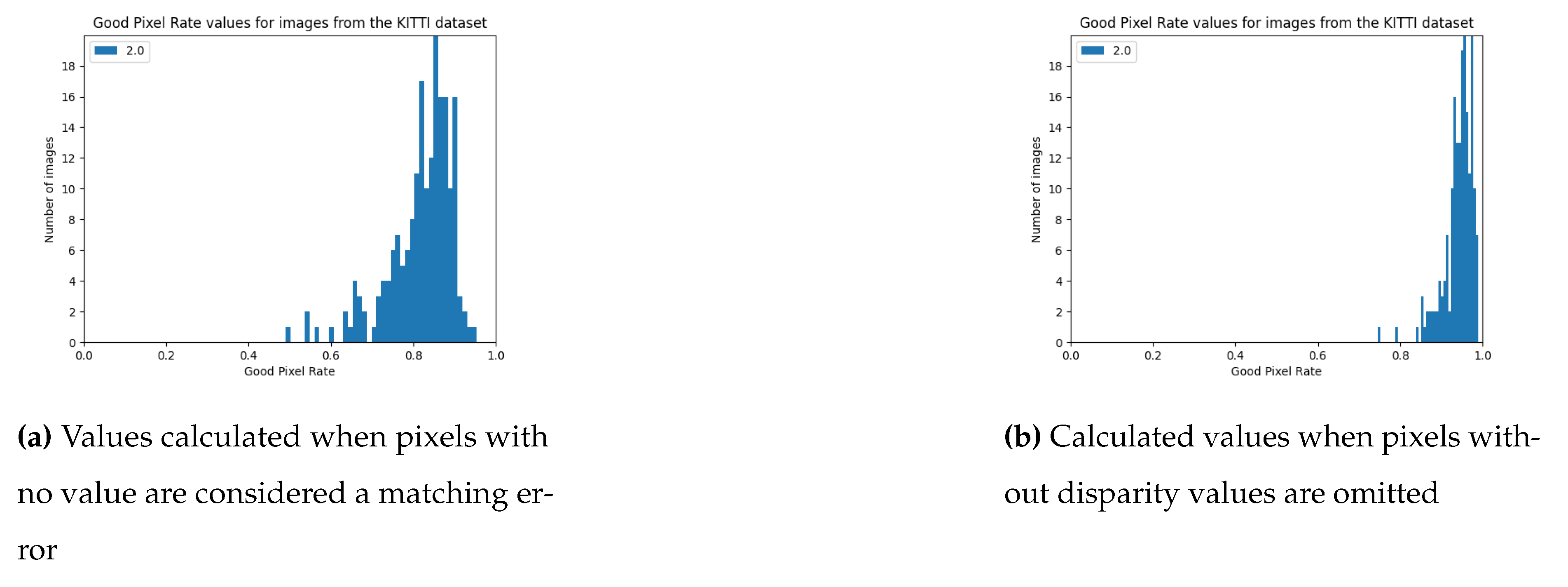
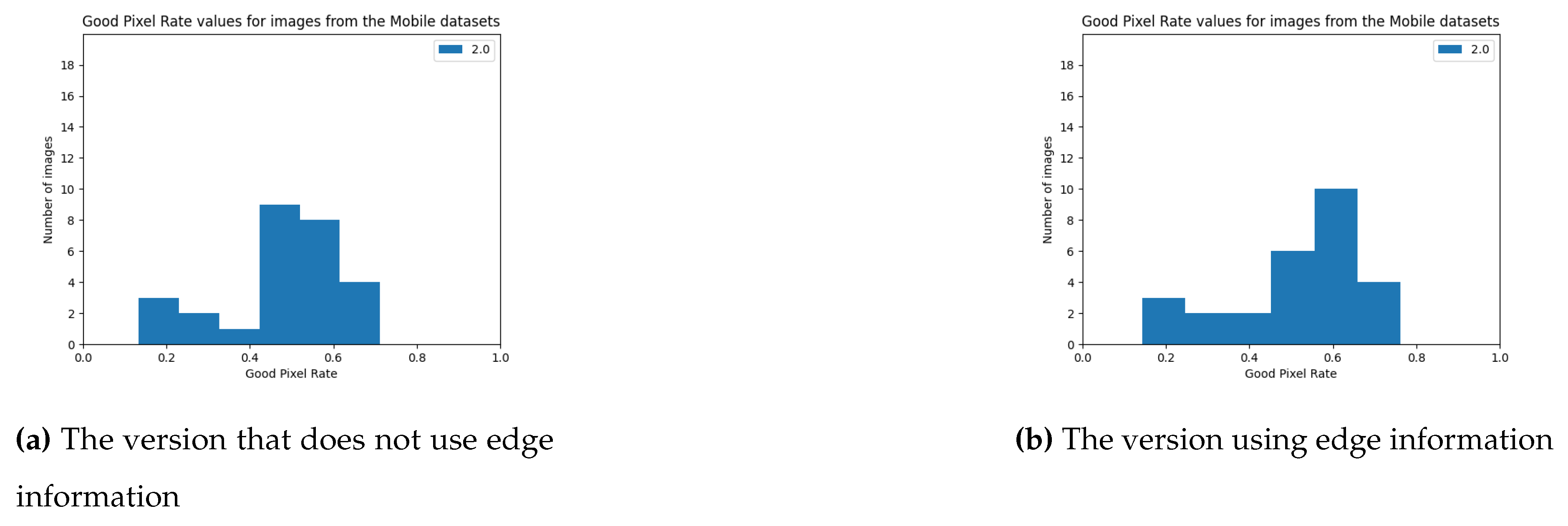
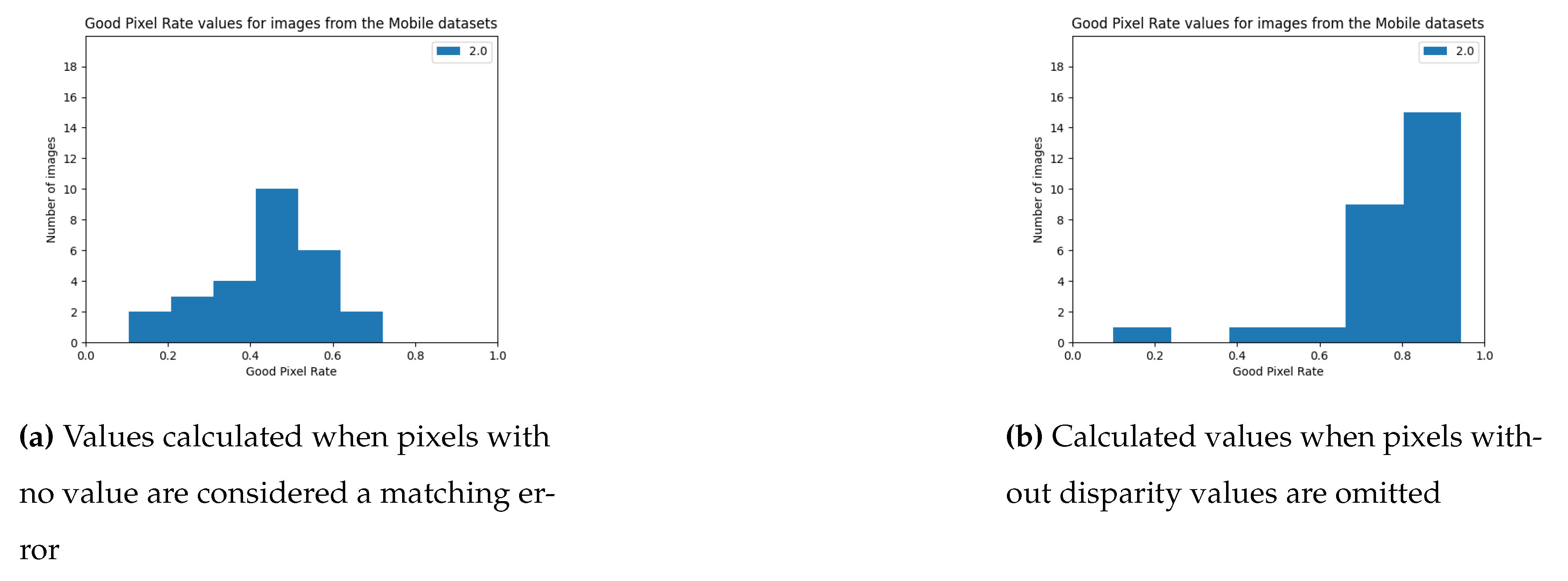
We tested the quality of the implemented algorithm using data from the KITTI and Middlebury 2021 mobile datasets described in this chapter. We used a package from the Stereo PCD library to assess the quality. We noticed that for the results for the data from both datasets, the error statistics differed significantly between image pairs, even when it came to image pairs from the same dataset. Therefore, we decided to present these results, in addition to tabulating the average error values, in the form of histograms showing the number of image pairs for which the error statistics were within a given range. We ran the tests for a number of parameter values and discuss the results for the best set of parameters found, for all images from the set we use the same parameter values.

We performed a similar experiment, using the same datasets as for our algorithm, for the SGBM [22] (Semiglobal Block Matching) algorithm from the OpenCV library, in which pixel matching is based on a smoothness constraint, which is usually expressed as a global cost function. SGBM performs fast approximation by optimizing paths from all directions.

In addition, because the SGBM algorithm does not compute a dense disparity map, but leaves pixels without values, we tested it in two ways - one in which pixels without values in the computed disparity map are not taken into account when calculating error statistics, and another in which such pixels are treated as false matches.

Tests on the KITTI set have shown that the implemented algorithm, with the same set of parameters, can achieve results that definitely differ in quality level. By increasing the tolerable error threshold, the number of pixels considered to be correctly matched increases, and the differences between the ratio of correctly matched pixels for different image pairs are minimally smaller. This is visible through the data in the Table 1.

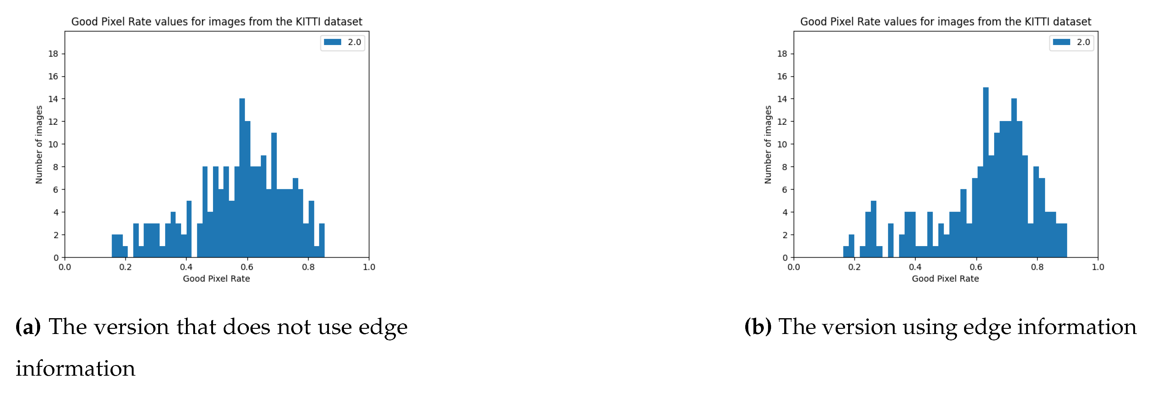
The version using the edge detection enhancement described in Section 3.2 achieved better results. Observing the histograms in Figure 9, it can be seen that there are few image pairs for which the algorithm achieved a very poor result.

In comparison, the SGBM algorithm for image pairs from the KITTI set achieves high results. Histograms showing the error statistics of pixel matches from a stereoscopic pair computed using the SGBM algorithm are in Figure 10.

Increasing the tolerable error threshold in the range for most pairs of images gives a significantly higher result, only for a few pairs of images the rate of correct matches increases little after raising the error tolerance threshold, this is observable on the data in the Table 1.

The algorithm from the Stereo PCD library gets worse results for the 2021 Mobile datasets than for the KITTI dataset. In the case of images from this set, it is also evident that the quality of the result strongly depends on the image pair - this is shown, among other things, by the histograms in Figure 11 and the data in the Table 2. Similarly, as with the results for the KITTI dataset, it can be seen that there are few image pairs for which the algorithm scored very poorly.

For the 2021 Mobile datasets, the SGBM algorithm also performs worse in quality tests than for the KITTI dataset. Histograms showing the ratio of correctly matched pixels for the data from this set can be found in Figure 10. As for the data from the KITTI set, increasing the threshold of acceptable error caused a noticeable increase in the value of the ratio of correctly matched pixels.

There are a lot of pixels without values on the calculated disparity maps - on average, about 44% of the pixels from the reference disparity map do not have their correspondents on the calculated disparity map. Recognizing such pixels as false matches results in significantly lower values of the rate of correct matches. Note, however, that this result can be easily improved by adding an additional step after executing the algorithm to fill the gaps in the calculated disparity maps, for example, using the values of pixels neighboring the gap.

In summary, the SGBM algorithm from the OpenCV library achieves better quality results than the algorithm from the Stereo PCD library. Moreover, the quality of the results for our algorithm definitely depends more on the input image pair. In the case of SGBM, there is also a similar dependence, but the differences in quality scores are much smaller.

3.4. Method of Performance Evaluation

To evaluate algorithms, one uses not only measures of the quality of the results obtained, but also, among other things, the time it takes to obtain it. Therefore, we also ran performance tests of the pixel-matching algorithm on a pair of stereoscopic images. We tested the processing time of the image pair using the time function from the time module of the standard Python language library. We ran the tests on a personal computer; the results may vary depending on the parameters of the machine on which they were run. Nonetheless, it allows to evaluate which algorithm runs faster and how the resolution of the images affects the running time of the algorithms. To make the results reliable, we ran the tests for different images from the collections and repeated them several times.

3.5. Performance Tests

The results obtained are shown in Table 3. In it, I compared two versions of the algorithm from the Stereo PCD library - a multithreaded one with all the proposed improvements from Section 2.1.2 and Section 2.1.3 and without the edge-related improvement, and the SGBM algorithm from the OpenCV library. The running times of the algorithms shown in the table were measured with the maximum disparity parameter set to 200 pixels.

The use of a constraint on the maximum value of disparity has resulted in similar matching times for images of the same resolution but with different orientations. This enhancement also improves the matching time by several times.

Significant speed-up was also achieved by using a multi-threaded version of the algorithm. Our Stereo PCD is faster than OpenCV algorithm, as depicted in Table 3.

4. Discussion

The goal of our research was to apply a method used in bioinformatics for aligning sequences of amino acids to the task of matching stereovision images. The experiments we conducted on publicly available datasets demonstrated the effectiveness and potential of this method for stereovision tasks. By setting appropriate parameter values for the break penalty value, we can obtain an accurate and smooth disparity map. Due to the fact that the lines are matched independently the obtained solutions are not optimal globally, but only optimal inside one pair of scanlines. For this reason, there are situations when the values of the of disparity in neighboring lines significantly deviate from each other despite the fact that a very similar fragment of the space.

In the next step of work on the presented algorithm, pixel matches from neighboring lines could be used so that the algorithm can force smoothness of the disparity in more than two directions, e.g., smoothness of a pixel in the direction of all its eight neighbors. This would require modifying the algorithm and proposing a matching function analogous to that for single-scanline matching. Such a solution will indeed increase the computational complexity of the algorithm, but will potentially achieve higher quality solutions.

Another potential way to improve the algorithm could be to try to speed up line matching. One potential way to this is to parallelize the computation. To do this, GPUs could be used and the dynamic programming algorithm could be implemented in a vector-based approach - simultaneously completing the cells of the auxiliary matrix located on the same antidiagonal. An alternative way to speed up the algorithm is to reduce the number of pixels comparing each other when matching lines. For this purpose, matches from neighboring lines can be used and the search space for a single pixel can be adaptively limited, with a full search applied only every few lines. Such an improvement of the algorithm will allow to reduce CPU consumption while matching the same number of frames per second as in the presented version, and thus application on small devices, i.e., embedded systems or mobile devices. Reducing the number of operations of the algorithm also makes it possible to increase the number of processed frames per second without changing the hardware, which could allow the algorithm to be applied to devices in motion, e.g., cars and real-time processing, depending on what speed-up is achieved, the algorithm could be used, for example, not only on roads in the city, but also on routes between cities.

In our opinion, the proposed algorithm can be used as a basis for creating more and better, both faster and more accurate, methods for fusing stereo-camera and lidar data.

5. Summary

A new algorithm for point cloud densification, for fusing lidar and camera. This algorithm was provided in the new open-source library named Stereo PCD, designed for Python 3. The library’s source code consists of about 1,700 lines of code, of which 1,000 lines are in Python and 700 lines in C++. It enables the processing of stereo image pairs and point clouds, e.g.,:

• creation of point clouds based on pairs of stereovision images and camera calibration data,
• combining several point clouds together,
• colouring of lidar point clouds based on camera images,
• saving point clouds containing point coordinates or coordinates with colour in formats that allow loading into a visualization tool MeshLab [23] or an object detector in a point cloud in three-dimensional space, e.g., OpenPCDet [24].

Moreover, the library includes a number of functions for determining extrinsic and intrinsic calibration matrices, projection matrices or distances between cameras based on various parameters.

The library provides support for the Middlebury 2021 mobile datasets [20], mentioned in Section 3.1.2, the KITTI Stereo dataset [21], depicted in Section 3.1.3.

The results show high performance and quality comparable with other top libraries.

References

- Shaukat, A.; Blacker, P.C.; Spiteri, C.; Gao, Y. Towards camera-LIDAR fusion-based terrain modelling for planetary surfaces: Review and analysis. Sensors 2016, 16, 1952. [Google Scholar]
- Ounoughi, C.; Yahia, S.B. Data fusion for ITS: A systematic literature review. Information Fusion 2023, 89, 267–291. [Google Scholar]
- Kolar, P.; Benavidez, P.; Jamshidi, M. Survey of datafusion techniques for laser and vision based sensor integration for autonomous navigation. Sensors 2020, 20, 2180. [Google Scholar]
- Singh, S.; Singh, H.; Bueno, G.; Deniz, O.; Singh, S.; Monga, H.; Hrisheekesha, P.; Pedraza, A. A review of image fusion: Methods, applications and performance metrics. Digital Signal Processing 2023, p. 104020.
- Lin, X.; Zhang, J. Segmentation-based filtering of airborne LiDAR point clouds by progressive densification of terrain segments. Remote Sensing 2014, 6, 1294–1326. [Google Scholar]
- Li, X.; Liu, C.; Wang, Z.; Xie, X.; Li, D.; Xu, L. Airborne LiDAR: state-of-the-art of system design, technology and application. Measurement Science and Technology 2020, 32, 032002. [Google Scholar]
- Heyduk, A. Metody stereowizyjne w analizie składu ziarnowego. Systemy Wspomagania w Inżynierii Produkcji 2017, Vol. 6, iss. 2.
- Lazaros, N.; Sirakoulis, G.C.; Gasteratos, A. Review of stereo vision algorithms: from software to hardware. International Journal of Optomechatronics 2008, 2, 435–462. [Google Scholar]
- McCarl, B.A.; Spreen, T.H. Applied mathematical programming using algebraic systems. Cambridge, MA 1997.
- Needleman, S.B.; Wunsch, C.D. A general method applicable to the search for similarities in the amino acid sequence of two proteins. Journal of molecular biology 1970, 48, 443–453. [Google Scholar]
- Tippetts, B.; Lee, D.J.; Lillywhite, K.; Archibald, J. Review of stereo vision algorithms and their suitability for resource-limited systems. Journal of Real-Time Image Processing 2016, 11, 5–25. [Google Scholar]
- Rusu, R.B.; Cousins, S. 3D is here: Point Cloud Library (PCL). IEEE International Conference on Robotics and Automation (ICRA); IEEE: Shanghai, China, 2011.
- John Stowers, S. Python Bindings to the Point Cloud Library. Last accessed 22.01.2024: https://strawlab.github.io/python-pcl/.
- Bradski, G. The openCV library. Dr. Dobb’s Journal: Software Tools for the Professional Programmer 2000, 25, 120–123.
- Scharstein, D.; Szeliski, R. A taxonomy and evaluation of dense two-frame stereo correspondence algorithms. International journal of computer vision 2002, 47, 7–42. [Google Scholar]
- Harris, C.; Stephens, M.; others. A combined corner and edge detector. Alvey vision conference. Manchester, UK, 1988, Vol. 15, pp. 10–5244.
- Nakamura, Y.; Matsuura, T.; Satoh, K.; Ohta, Y. Occlusion detectable stereo-occlusion patterns in camera matrix. Proceedings CVPR IEEE Computer Society Conference on Computer Vision and Pattern Recognition. IEEE, 1996, pp. 371–378.
- Scharstein, D. Middlebury stereo page. Last accessed 04.01.2024: http://vision.middlebury.edu/stereo/data, 2001.
- Geiger, A. Kitty dataset page. Last accessed 09.01.2024: https://www.cvlibs.net/datasets/kitti/, 2012.
- Scharstein, D.; Hirschmüller, H.; Kitajima, Y.; Krathwohl, G.; Nešić, N.; Wang, X.; Westling, P. High-resolution stereo datasets with subpixel-accurate ground truth. Pattern Recognition: 36th German Conference, GCPR 2014, Münster, Germany, September 2-5, 2014, Proceedings 36. Springer, 2014, pp. 31–42.
- Geiger, A.; Lenz, P.; Urtasun, R. Are we ready for autonomous driving? the kitti vision benchmark suite. 2012 IEEE conference on computer vision and pattern recognition. IEEE, 2012, pp. 3354–3361.
- Hirschmuller, H. Stereo processing by semiglobal matching and mutual information. IEEE Transactions on pattern analysis and machine intelligence 2007, 30, 328–341. [Google Scholar]
- Cignoni, P.; Callieri, M.; Corsini, M.; Dellepiane, M.; Ganovelli, F.; Ranzuglia, G. MeshLab: an Open-Source Mesh Processing Tool. Eurographics Italian Chapter Conference; Scarano, V.; Chiara, R.D.; Erra, U., Eds. The Eurographics Association, 2008.
- Team, O.D. OpenPCDet: An Open-source Toolbox for 3D Object Detection from Point Clouds. https://github.com/open-mmlab/OpenPCDet, 2020.