Preprint
Article

Continental regional flood frequency analysis: combining enhanced datasets and a Bayesian framework

Altmetrics

Downloads

112

Views

54

Comments

0

A peer-reviewed article of this preprint also exists.

Submitted:

08 July 2024

Posted:

10 July 2024

You are already at the latest version

Alerts
Abstract
Flood frequency analysis at large scales, essential for the development of flood risk maps, is hindered by the uncertainty in outputs of process-based hydrological models and the scarcity of gauge flow data. We develop a Bayesian hierarchical model (BHM) based on the Generalized Extreme Value (GEV) distribution for regional flood frequency analysis at high resolution across North America. Our model leverages annual maximum flow data from ≈20000 gauged stations and a dataset of 130 static catchment-specific covariates to predict extreme flows at all catchments over the continent as well as their associated statistical uncertainty. Additionally, a modification is made to the data layer of the BHM to include daily gauge discharge data when available, which improves the precision of the discharge level estimates. We validated the model using a hold-out approach and found that its predictive power is very good for the GEV distribution location and scale parameters and improveable for the shape parameter, which is notoriously hard to estimate. The resulting discharge return levels yield satisfying agreement when compared with available design peak discharge from various government sources. Assessment of the covariates’ contributions to the model also informs on the most relevant underlying factors influencing flood-inducing peak flows. The key covariates in our model are temperature-related bioindicators, the catchment drainage area and geographical location.
Keywords: 
Subject: Environmental and Earth Sciences  -   Water Science and Technology

1. Introduction

Flooding is one of the most impactful natural disaster in term of human, economic and financial damage worldwide [1]. The risk of increasingly impactful and damaging widespread flood events is further exacerbated by the changes in hydrological cycles induced by global warming [2,3].
Flood frequency analysis is an essential field of study in hydrology which concerns the estimation of peak flow levels corresponding to a certain return period, defined as the average time between occurrences of an extreme event. Such information on high flow events is useful in many settings such as dam design for flood protection, reservoir design and management, ecology management and river pollution control [4]. For flood risk assessment, the estimated peak flows can serve as input to a hydraulic model to simulate possible overflowing of river banks onto nearby floodplains and measure the inundation depth and extent. This could lead to the development of flood risk maps, informing on potentially vulnerable flood-prone areas. Thus, ideally extreme streamflow levels in all areas of interest need to be estimated with precision.
If all locations of interest had observed data available, this estimation problem could simply be performed statistically by fitting a probabilistic distribution to the time series of observed discharge and deriving the extreme discharge values. Common distributions used to model extreme streamflows are the Gumbel, Generalized Extreme Value (GEV), Generalized Pareto (GP), Log-Pearson type III, Log-normal and Laplace distributions [5,6]. Estimating high discharge values from observed time series comes with inherent uncertainty attributed to the essentially rare occurrence of extreme events [7].
In reality, river gauges are only available in a small subset of locations, due to limited resources. Estimating river flows in ungauged catchments remains one of the most complex challenges in catchment hydrology [8]. One possible solution, sometimes called the indirect method, involves using rainfall data fields (from climate reanalysis products or downscaled climate models) to run rainfall-runoff models and simulate synthetic flows homogeneously over an entire geographical area. However, these synthetic flows are not point estimates but mean values averaged over a grid box. As such, they are usually accompanied with substantial uncertainty, stemming from their coarser resolution, the parameterization of the rainfall-runoff model [9] and the uncertainty in the rainfall field itself [10].
This motivates the use of spatial data-driven models to interpolate discharge values in ungauged areas from nearby gauged basins. This field named regional flood frequency analysis (RFFA) traditionally uses the index flood method [11] to infer extreme peak flow in ungauged locations from similarly behaving gauged basins. In this method, the region of interest is divided into hydrologically homogeneous subregions using data-driven pooling or expert knowledge. A single frequency curve is then fitted to the observed discharge values in each subregion, which is then rescaled with location specific flood indexes. Although this method remains fairly popular in the hydrology community, its simplicity has raised criticism [12] and often does not account for the full hydrological complexity within each subregion. The underlying assumption that each subregion has a common regional flood frequency curve is also not rigorously verified [12]. Moreover, the partitioning into subregions can be arbitrary and contributes to increase uncertainty in the model [13].
Alternatively, Bayesian hierarchical models (BHM) are a class of latent variable model which is suitable for data which follows a certain hierarchical structure [14]. This structure is embedded in the model using a latent process layer, where hyperparameters are introduced to share information from different data subgroups. In RFFA, data is organized spatially (grouped by stations) but also temporally (grouped by time of measurement). The use of the Bayesian framework is advantageous for multiple reasons. Because all model parameters are estimated simultaneously, uncertainty is taken into account across the whole modeling chain and is directly provided as a by-product of the model. This is beneficial for analyzing extreme flood data in general, especially when the need to quantify flood uncertainty is emphasized [15]. Furthermore, by pooling information from gauged data across all locations, the BHM mitigates the negative effects of locations with short data records, because data sharing allows estimation in these locations to borrow strength from other data-rich stations [14].
Bayesian hierarchical models have been used extensively and with success in RFFA [12,15,16,17,18,19,20]. Some studies incorporate spatial information using gaussian random fields to correlate flood describing parameters in the latent process [12,16,21]. Oftentime, regression-based techniques are integrated inside the BHM to link streamflows to suitable covariates and allow prediction of extreme floods at ungauged catchments. For example, [17] and [22] use the drainage area as the main predictor which scales with the location and scale parameters of the GEV distributions used to describe discharge observations. Non-stationarity in time can also be embedded as part of the BHM model if such assumptions are justified, as is the case in [18], where peak flow event durations are allowed to vary temporally. The studies mentioned above usually limit their geographical application to a river basin [16,17], a region [23] or a small country (the UK [20], Norway [19]).
Finally, we note that non-linear machine learning and deep learning models are progressively gaining popularity as a promising tool to perform RFFA [24,25,26,27]. Most of these studies utilize at-site flood frequency analysis to derive design flood values at gauged stations, then use a machine learning model to predict design flood values at ungauged stations. One of the main drawbacks of this approach is that extreme value theory is not leveraged to extrapolate to unseen extreme events, so the prediction of discharge levels corresponding to very high return periods can be inaccurate. Furthermore, standard machine-learning based models do not explicitly account for the statistical uncertainty, even though attempts to remedy this problem have been made for RFFA using Bayesian networks [28].
We bring several new methodological extensions to the standard Bayesian hierarchical model to perform regional flood frequency analysis in all catchments across North America and take advantage of the enhanced data quality and quantity collected. The scale of our study is continental, using substantially more gauge data and covariates than previous similar studies. A set of enriched 130 catchment specific covariates are used inside the BHM to describe the GEV distribution parameters. This constitutes a predictive model which can be used to estimate extreme discharge levels at all ungauged catchments, using extracted information from the gauge stations. To our knowledge, previous studies using a regression approach for RFFA were limited to less than 20 catchment descriptors, providing only a simplified description of catchment hydrology. By analyzing the regression coefficients estimated for each variable, we are also able to assess and classify their relevance for predicting extreme fluvial peak flows.
Second, to improve the precision of estimates, a modification is made to the data layer likelihood which allows using both annual maxima and daily discharge data whenever available. This increases the amount of high quality data for the subgroup of stations where daily data is available and reduces model uncertainty. Annual maxima are modeled with the GEV distribution and peaks over threshold extracted from daily data are modeled with the GP distribution. Both stem from the extreme value theory, where they are proven to be the asymptotic form for the distributions of extreme random variables [7]. For the shape parameter of the GEV and GP distributions, the sign of its value determines the upper tail decay behavior, giving the model enough flexibility to cover a wide range of flood regimes [6].

2. Materials and Methods

2.1. Data

2.1.1. Discharge Data

Annual maximum discharge time series (in m   3 / s) come from USGS National Water data for the USA [29] and HYDAT Database for Canada [30]. The combined annual maximum peak flow dataset covers 23283 stations with at least 10 years of record. Daily discharge data comes from various sources, including The Global Runoff Data Centre database (GRDC) [31], USGS National Water data [29], Ministère de l’Environnement et de la Lutte contre les changements climatiques [32] and Water survey of Canada [30]. Daily data was preprocessed to select only the stations deemed reliable. This is done by comparing annual maxima extracted from the daily series to the corresponding annual maxima dataset. Mean relative error is calculated across concurrent annual maxima for each station. Stations with a mean relative error lower than 10 % for at least 10 years of data are considered reliable. Finally, we discard stations with a drainage area lower than 50 km   2 and any station-year with non-complete daily data. This pre-processing step results in 3385 stations with daily discharge data and 19963 stations with annual maximum discharge data over North America. The locations of the stations with only annual maximum discharge available and both type of data available are displayed in Figure 1 by blue and red dots respectively. As expected, the gauge network is dense in the United States (US) and sparser in Canada, especially in the northern latitudes. No Mexican data was used in this study. In southern Quebec, the majority of annual maximum observations are in fact pseudo-observations stemming from an interpolation method used by the provincial government [33], which explains the disproportionately high density of data in this area.

2.1.2. Catchment Delineation

The North American continent is divided into 14 hydrologically similar regions corresponding to level 2 of the HydroBASINS product [34]. These regions are named and numbered, in order: 1- Arctic, 2- Northwest passage, 3- Hudson bay, 4- Nunavut, 5- North-western territories, 6- Alaska, 7- Saint-Lawrence, 8- Prairie, 9- British Columbia, 10- East Coast, 11- Midwest, 12- California, 13- Mexico and 14- Carribean. They are shown in Figure 1.
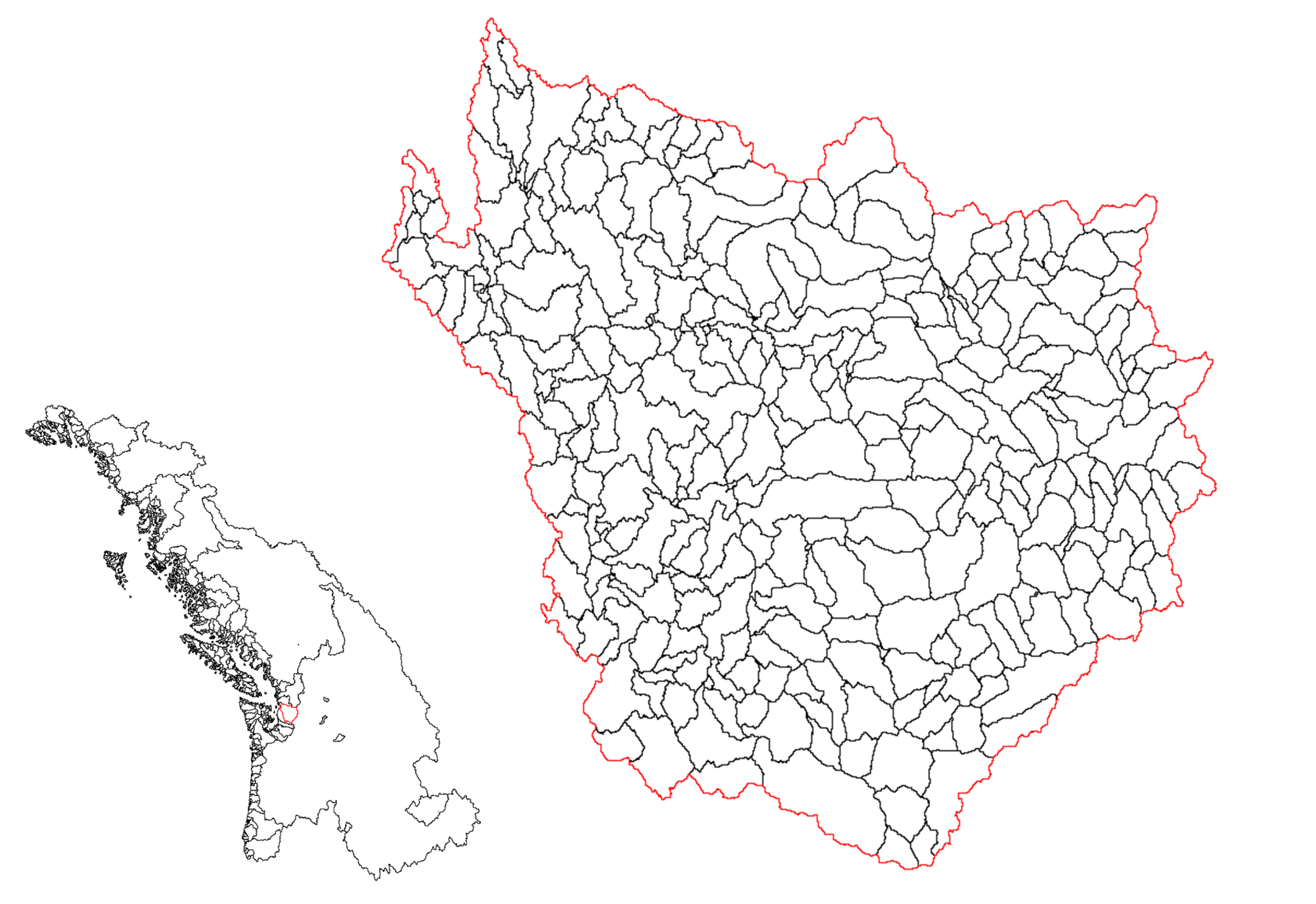
The HydroBASINS regions are further partitioned into 1.8 million unit catchments with an average size of 10 km   2 , following the methodology described below. The 90m MERIT-HYDRO Digital Elevation Model [35] is first used to derive the flow direction raster and compute the flow accumulation raster. Watershed delineation is performed for each basin identified within the DEM, employing a threshold of 10 km   2 . The delineation process involves specific functions within the Arc Hydro Toolbox [36], following a classic watershed delineation approach, namely: StreamDefinition, Stream Segmentation, CatchmentGridDelineation, CatchmentPolygonProcessing, and DrainageLineProcessing. Using functions within the Arc Hydro Toolbox allows for precise attribution of each line to its respective catchment, effectively ensuring its connections with downstream features. This delineation results in a comprehensive collection of 14246 network groups (NetID), further divided into 1821571 catchments (COMID). Streamflows in our model are modeled at the unit catchment scale. Figure 2 shows the delineation of HydroBASINS region 9, British Columbia, into river networks (left) and unit catchments (right), for illustrative purposes.
Finally, gauged station locations are used to map each station to its respective catchment within the river network. Discrepancies between the actual station position and the reported one are quite common. To mitigate this, the differences between the reported station drainage area and the cumulative upstream drainage area of nearby basins are inspected. The station is then matched with the catchment with the smallest difference error.

2.1.3. Catchment Attributes

A large dataset of 130 static covariates for all identified catchments across North America is used to model extreme discharge at ungauged catchments. These covariates describe catchment characteristics in term of geography (latitude, longitude, elevation), hydrology (average stream slope, drainage length, drainage area, flow direction fraction), climatology (solar radiation, temperature and precipitation, wind speed, vapor pressure) and soil/land properties (silt, sand, clay and gravel fraction of different soil layers, fractional coverage of different land coverage classes, mean base saturation). The complete description of each attribute as well as its source is presented in Table S1 of the Supplementary Information. Prior to applying the model, all covariates are quantile-transformed to follow the gaussian distribution.

2.2. Methodology

2.2.1. Extreme Value Theory

Following the standard methodology described in [7], extreme discharge values are extracted for statistical analysis from the original datasets. Since annual maximum discharges are already extreme, we only need to extract high daily peak flows. For stations where daily discharge is available, excesses over the 0.98th quantile threshold are selected followed by a declustering step with the run method, where the run length is chosen as 3 days [7]. This assumes that high flow events are temporally separated by at least 3 days. Station daily data are discarded prior to analysis if less than 10 high flow events are identified.
In accordance with the extreme value theory, we use the Generalized Extreme Value (GEV) distribution and the Generalized Pareto (GP) distribution to model the annual maxima and excesses over threshold data respectively. The cumulative distribution function of the GEV distribution is given by:
F G E V ( x ; μ , σ , ξ ) = exp 1 + ξ x μ σ 1 ξ
where μ , σ , ξ are the location, scale and shape parameters respectively. The sign of the shape parameter determines the upper tail decaying speed of the underlying data. If ξ < 0 , the distribution is bounded on the right. If ξ > 0 , the right tail decays with a power function rate and the distribution is heavy tailed. If ξ = 0 , the GEV distribution becomes a Gumbel distribution, where the decaying rate of the upper tail is exponential.
The cumulative distribution function of the GP distribution is given by:
F G P ( z ; σ , ξ ) = 1 1 + ξ z σ 1 ξ
where σ and ξ are respectively the scale and shape parameters. The shape parameter of the GP distribution can be interpreted in the same way as for the GEV distribution. In fact, the two distributions arise from two different ways of looking at extreme data, and there is a natural correspondence between their parameters [7]:
σ G P D = σ G E V + ξ G E V ( u μ G E V )
ξ G P D = ξ G E V
where u is the threshold used to define the excesses. For an introduction to extreme value theory, the reader can refer to [7].

2.2.2. Bayesian hierarchical model

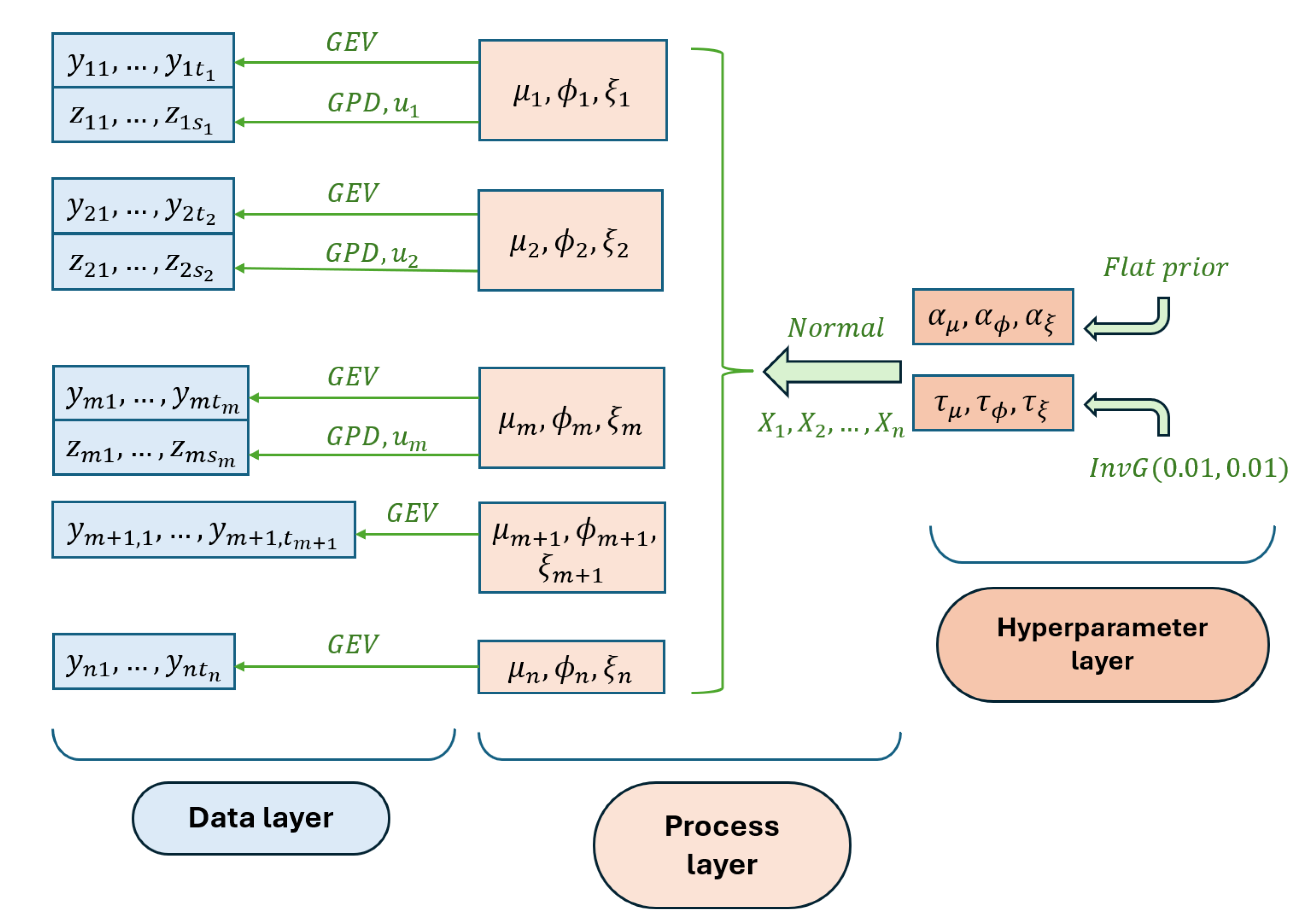
The annual maximum peak flows and high excesses over threshold extracted from the daily data are used as input to the Bayesian hierarchical model (BHM). According to the Bayesian paradigm, all model parameters are themselves viewed as probabilistic distributions to be estimated. Classically, a BHM comprises three hierarchical layers: the data layer, the latent process layer and the hyperparameter layer. The structure of our model is summarized in Figure 3.
We start by describing the data layer, where discharge data is modeled probabilistically. For simplicity, assume that all stations are indexed from 1 to n, and that stations from 1 to m contain both annual maxima and excesses over threshold data, where m n . Then the data layer is described by the following equations:
y i = ( y i 1 , , y i t i ) G E V ( e x p ( μ i ) , e x p ( ϕ i ) , ξ i ) i = 1 , , n
z j = ( z j 1 , , z j s j ) G P D ( σ j , ξ j ) j = 1 , , m
σ j = e x p ( ϕ j ) + ξ j ( u j e x p ( μ j ) )
where y i t is the annual maximum for station i in year t and z j s is the s t h excess over the threshold u j of station j. Here we parameterize the GEV distribution with the logarithm of the location and scale parameters, so as to ensure their positivity when performing linear regression. This is necessary for the scale parameter by definition, and desirable for the location parameter, since discharge values are greater than zero. Therefore, ( μ i , ϕ i , ξ i ) are the log-location, log-scale and shape parameters of the GEV distribution for station i, respectively. We take advantage of the close relationship between the GEV and GP distributions to express the GP distribution parameters with the GEV distribution parameterization. This allows sharing of information for stations where both annual maxima and daily discharge data are available and reducing uncertainty when estimating the GEV distribution parameters. Notice that the latter are space-varying but not time varying. In our model, discharge extremes are considered stationary over the historical period.
The latent process layer links the site-specific GEV distribution parameters together through a linear regression model. It is described as follows:
μ i N ( X i T α μ , τ μ 2 ) i = 1 , , n
ϕ i N ( X i T α ϕ , τ ϕ 2 ) i = 1 , , n
ξ i N ( X i T α ξ , τ ξ 2 ) i = 1 , , n
where N denotes the normal univariate distribution and X i R p is the vector of p = 131 covariates for station i. The first element of X i is 1, which accounts for the intercept term. For the log-location GEV distribution parameter, α μ R p is the regression coefficient vector and τ μ 2 R is the variance parameter. The same applies to α ϕ , α ξ , τ ϕ 2 , τ ξ 2 . The regression coefficients ( α μ , α ϕ , α ξ ) are shared across all sites. The distributions of the hyperparameters { ( α k , τ k 2 ) , k { μ , ϕ , ξ } } are specified in the hyperparameter layer. Since we have sufficient data to accurately estimate the model parameters, hyperparameters are assumed to follow uninformative prior distributions to avoid introducing bias in the model:
α k 1 k { μ , ϕ , ξ }
τ k 2 I n v G ( 0.01 , 0.01 ) k { μ , ϕ , ξ }
where I n v G denotes the inverse Gamma distribution.
The developed Bayesian hierarchical model is applied to each HydroBASIN region independently. This means that the regression parameters described above are region-specific. This assumption is motivated by considering that catchments inside each HydroBASIN region are hydrologically more similar, while catchments from different regions might exhibit distinct hydrological regimes.

2.2.3. Inference at Gauged Stations

The joint posterior distribution of the modeled parameters, conditioned on the discharge data y = ( y 1 , , y n ) , z = ( z 1 , , z m ) and on covariate data X = ( X 1 , , X n ) can be expressed as:
f p o s ( θ y , z , X ) = i = 1 n t = 1 t i G E V ( y i t e x p ( μ i ) , e x p ( ϕ i ) , ξ i )
× j = 1 m s = 1 s j G P D ( z j s e x p ( ϕ j ) + ξ j ( u j e x p ( μ j ) ) , ξ j )
× k = 1 n N ( μ k X k T α μ , τ μ 2 ) N ( ϕ k X k T α ϕ , τ ϕ 2 ) N ( ξ k X k T α ξ , τ ξ 2 )
× I n v G ( τ μ 2 0.01 , 0.01 ) I n v G ( τ ϕ 2 0.01 , 0.01 ) I n v G ( τ ξ 2 0.01 , 0.01 )
where θ encompasses the GEV distribution parameters and hyperparameters ( α k , τ k 2 ) , k { μ , ϕ , ξ } . Here G E V , G P D , N , I n v G denote the GEV, GP, Normal and inverse Gamma probability distribution functions, respectively. Lines (11) and (12) of the equation correspond to the data layer and denote the GEV and GP likelihood functions. Line (13) corresponds to the latent process layer with the regression terms incorporated inside a gaussian likelihood function. Finally, line (14) corresponds to the hyperparameter prior distributions.
We use Monte-Carlo Markov chain (MCMC) simulation methods [37] to sample from the joint posterior distribution of the parameters. The chosen sampler is a Metropolis-within-Gibbs algorithm, where inside the structure of a Gibbs sampler, Metropolis Hastings steps are used whenever a conditional distribution can’t be sampled trivially. Specifically, the Metropolis Hastings algorithm is employed to sample new values for the GEV distribution parameters, using a random walk procedure for the value proposals. An adaptive mechanism is used to finetune the step size of the random walk distributions every 50 MCMC iterations, following the ideas in [38]. This allows good mixing of the posterior parameter chains, with acceptance rates for GEV distribution parameters around 0.44 [39]. The adaptive Metropolis-within-Gibbs MCMC algorithm is run for 30000 iterations, where the first half is used as the burn-in period, with a thinning of 10 iterations before obtaining the posterior joint distribution chains. For gauged stations, GEV distribution parameters are readily obtained from the corresponding posterior MCMC samples. Subsequently, the posterior distribution of the extreme discharge levels can be calculated from the MCMC samples by inverting the GEV cumulative distribution function, for a range of quantiles/return periods.

2.2.4. Prediction in Ungauged Catchments

The GEV distribution parameters for ungauged catchments are derived using the estimated regression coefficients and ungauged catchment covariates. Specifically, for k { μ , ϕ , ξ } and for ungauged catchment u, the posterior predictive distribution of k u is
f p r e d ( k u | y , z , X ) N ( X u T α k , τ k 2 ) f p o s ( α k , τ k 2 y , z , X ) d α k d τ k 2
where f p o s ( y , z , X ) is the posterior distribution. From the sampled posterior distribution of the regression and variance parameters, we easily obtain a sample of the posterior predictive distribution for the GEV parameters of ungauged catchments. This is done using the following procedure. Denote m = 1 , , M the MCMC posterior samples and α k ( m ) , τ k 2 ( m ) ; k { μ , ϕ , ξ } the mth sample of the regression and variance parameters. Then we independently sample
k u ( m ) N X u T α k ( m ) , τ k 2 ( m ) for m = 1 , , M ; k { μ , ϕ , ξ }
for catchment u. Then similarly to gauged stations, predictive distributions of extreme discharge levels corresponding to a range of return periods can be calculated, informing on the most probable values but also the uncertainty surrounding the estimated return levels.

3. Results

Since gauge density is very sparse in regions 1 to 4 (Northern Canada) and 12 to 14 (substantial overlap with Mexico), as seen in Figure 1, we focus our attention on regions 5 to 11, which also cover the majority of major population hubs. Therefore, results will be presented for these regions, with some results presented in detail for region 9, British Columbia.

3.1. Model Validation

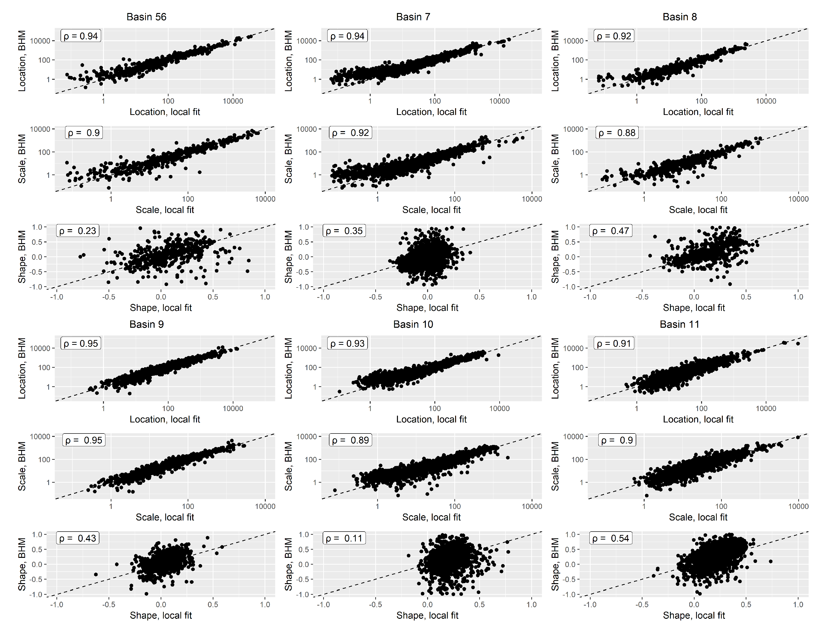
To validate the ability of the model to capture spatial patterns in flood extremes and generalize to unseen data, we train it on half of the stations and validate the results on the remaining half, following a hold-out approach. We do so by predicting the GEV distribution parameters at validation stations as if they were ungauged, then comparing those estimates to the locally estimated GEV distribution parameters. The local fit is performed using maximum likelihood estimation. Because the number of stations in regions 5 and 6 is lower than other regions, they are merged and used together as an unique region, meaning that a single BHM is fitted for the combined region 5-6 during the validation procedure. Results for this hold-out validation approach are presented for regions 5 to 11 in Figure 4. Overall, the GEV location and scale parameters predicted by the BHM model agree well with the locally estimated location and scale parameters for all regions. For regions 5 to 8, we observe a slight tendency of the BHM to overestimate the location and scale values for small streams, a behavior not reproduced in regions 9 to 11. This might be due to a sparser gauge network in northern areas compared to southern ones, providing less data for the model to accurately learn the flood extreme patterns in small rivers. Generally, these two parameters are reasonably well estimated by local maximum likelihood methods when the recorded annual maxima series is of a reasonable length. This asserts the ability of the BHM model to regionalize the location and scale of flood extremes using the covariates. The latter are able to account for the variability in these two parameters, as shown by the goodness-of-fit of the comparison (Pearson’s correlation of 0.88 and above for all regions). For the shape parameter, the estimates from the BHM model agree much less with those from the local models, with Pearson’s correlations varying from 0.11 to 0.54. This can be due to various reasons:
  • the BHM regression model can only capture a fraction of the variability of the GEV shape parameter. The unexplained random error remains quite substantial which makes out-of-sample predictions noisy. This same observation has been reported in the past literature [40].
  • the shape parameter is notoriously difficult to estimate accurately [15,41], especially when fitting local models to data records of limited length. Therefore, the local estimates of the shape parameters may themselves be inaccurate.
For the shape parameter, agreement between the BHM and the local model is stronger for regions 8, 9 and 11, suggesting that the quality of its prediction is not linked to the gauge network density in each region but the ability of the covariates to capture variations in regional shape patterns.
Next, the regression errors (residuals) are assessed for the three GEV distribution parameters and for all stations. They are taken as the mean of the posterior distribution of regression errors, for each GEV distribution parameter k { μ , ϕ , ξ } and for each site i:
ϵ k , i = 1 M m = 1 M k i ( m ) X i T α k ( m ) i = 1 , , n ; k { μ , ϕ , ξ }
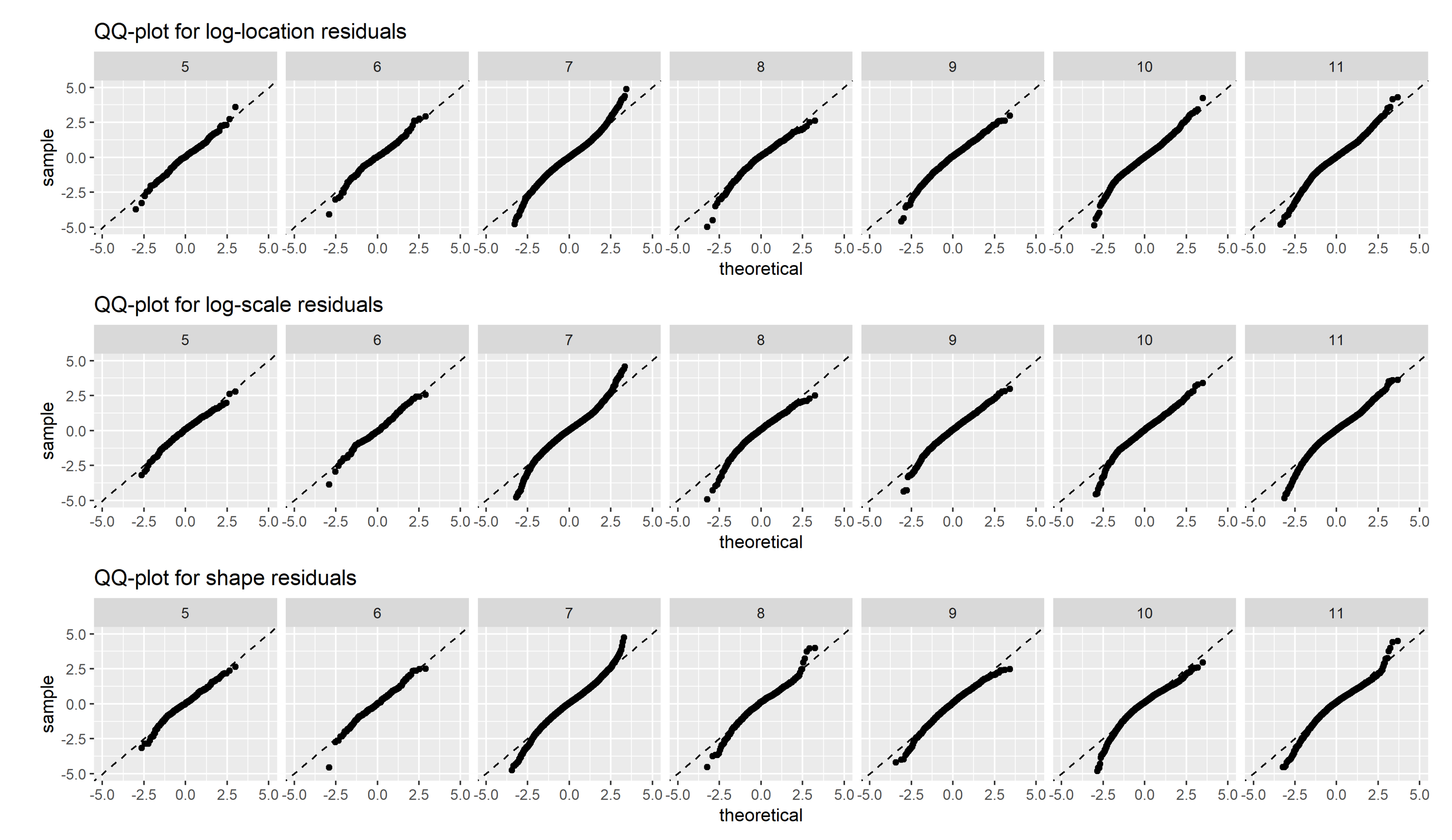
where notations follow those used in Section 2.2.2. Our BHM model assumes the residuals to be gaussian random noises. Their normality is evaluated using normal quantile-quantile plots, as shown in Figure 5.
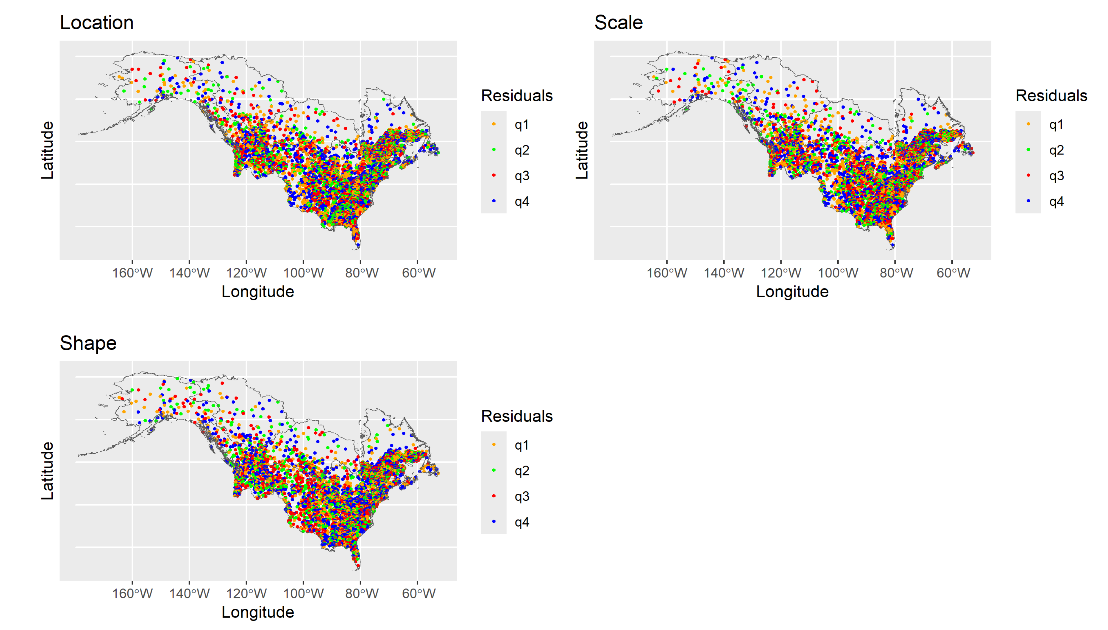
If the residuals are perfectly normal distributed, points are located on the diagonal line. The normality assumption is a reasonable simplification for the three parameters, although the lower tails are slightly heavier than normal for regions 7 to 11. To assess their spatial independence, residuals are plotted spatially in Figure 6, grouped into four categories (q1, q2, q3 and q4) splitted according to the first, second (median) and third quartile. There is no clear spatial pattern discernable in the regression residuals for all three GEV distribution parameters. This finding justifies not using an explicit spatial random field for the regression residuals, which adds a layer of complexity to the model at the cost of its scalability.

3.2. Model Results

3.2.1. Covariate Importance

Since all covariates are on the same scale after quantile transformation, the regression coefficients can be compared to evaluate covariate importance. For each region and GEV distribution parameter, we follow the procedure below to classify covariates:
  • coefficients are first rescaled to [ 1 , 1 ] by dividing by the highest absolute coefficient value. This removes the regional variability of the regression coefficient values.
  • all covariates with the regression coefficient posterior distribution containing 0 inside its 0.1th and 0.9th quantiles are discarded. Therefore, only coefficients considered significantly different from 0 are considered.
  • the remaining covariates are classified according to the absolute value of the estimated regression coefficient mean value.
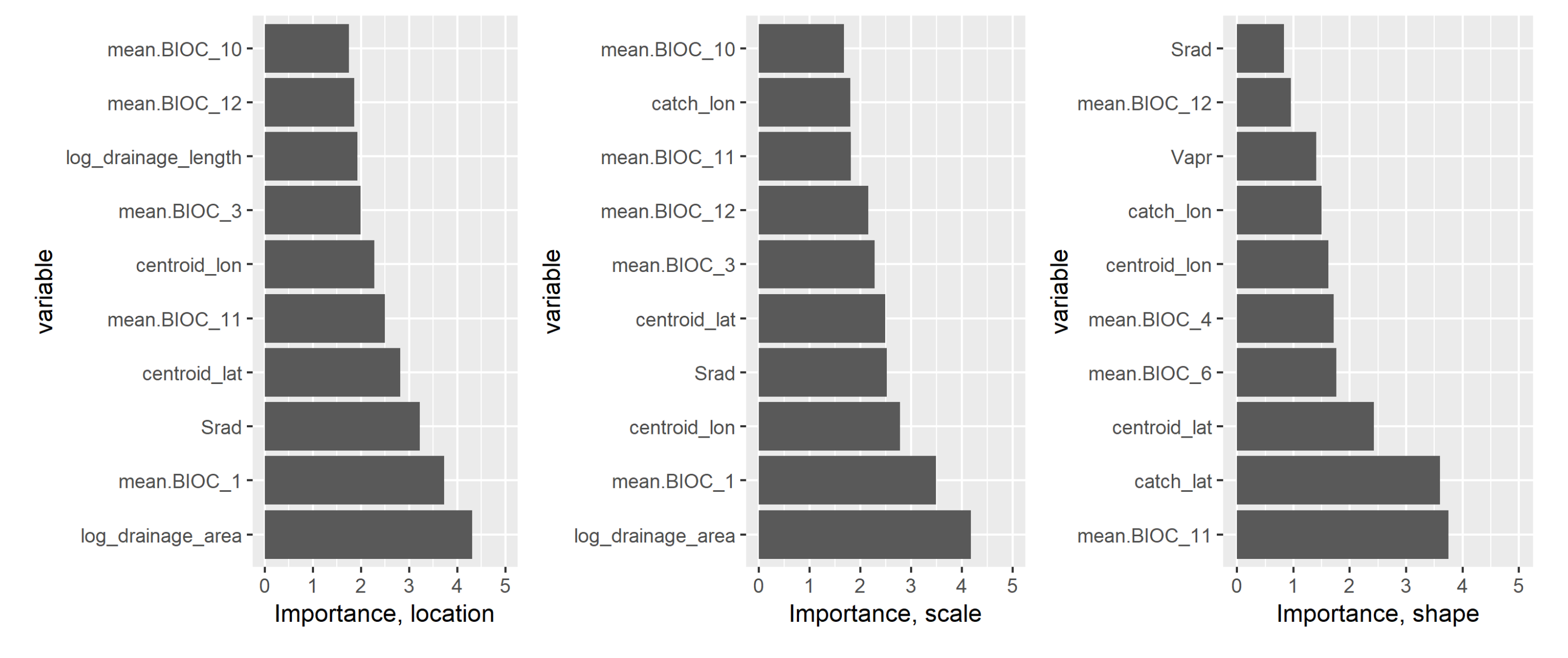
Then for each GEV distribution parameter and covariate, an aggregated importance score is defined by summing the absolute value of the corresponding regression coefficients across regions 5 to 11. If a variable was discarded during the previous steps, its corresponding coefficient value is taken as 0. This importance score is then used to rank the variables. The result of this ranking is shown in Figure 7 where for each GEV distribution parameter, the top ten variables are shown along with the value of its importance score.
The drainage area is the most significant variable for predicting the location and scale parameters, confirming the scaling rule of the latter with the drainage area identified in the literature [16,17,42]. It is absent from the top variables for the shape parameter, which tallies with the former authors’ conclusions that this scaling relationship is not supported for the shape. For the location and scale parameters, the most relevant variables are similar: the drainage area is closely followed by the annual mean temperature (mean.BIOC_1), solar radiation and the location of the centroid of the catchment’s drainage area (centroid_lat and centroid_lat). Temperature-related bioindicators are very significant in our model for predicting peak flows, with four of them present in the top ten variables for both the scale and location parameters: apart from mean annual temperature, the other relevant covariates are the mean temperature of coldest quarter (mean.BIOC_11), isothermality (mean.BIOC_3) and the mean temperature of warmest quarter (mean.BIOC_10). For the shape parameter, the most significant variables are the mean temperature of coldest quarter (mean.BIOC_11) and the catchment and drainage area centroid latitudes.
It is somewhat surprising that temperature related bioindicators are more relevant for predicting extreme discharge in our model than precipitation related bioindicators (mean.BIOC_12 to 19), since we expect a close and direct relationship between precipitation and streamflows. This might be because the precipitation related covariates in our dataset are mean values over a month or a quarter, which might behave differently from precipitation extremes. Previous studies already pointed out that trends in extremes are certainly of a different nature than those of the bulk of the distribution [43]. Albeit, annual precipitation (mean.BIOC_12) is a significant covariate for all three parameters. Interestingly, another study applying machine-learning techniques to predict fluvial flood quantiles in India also found temperature related variables to be more important than precipitation related ones [27].
Geographical location is an important factor in predicting all three parameters. The latitude is ranked much higher than longitude for the shape parameter, indicating that the tail behaviour of fluvial floods presents the largest variability in the north-south direction. Second, the location of the centroid of upstream drainage area (centroid_lon and centroid_lat) is ranked higher for the location and scale parameters while the location of the catchment (catchment_lon and catchment_lat) seems to be more relevant for the shape parameter. This can in part translate the fact that the location and scale of extreme streamflows are reasonably well described at the watershed scale, while the shape parameter has more pronounced local geographical variations.
To sum up, the most important covariates for predicting extreme discharges in our model are geographical location, temperature-related bioindicators and for the bulk of the distribution, the drainage area. A more detailed ranking of the covariates by region is presented in figure S2 of the supplementary information.

3.2.2. Estimated GEV Distribution Parameters

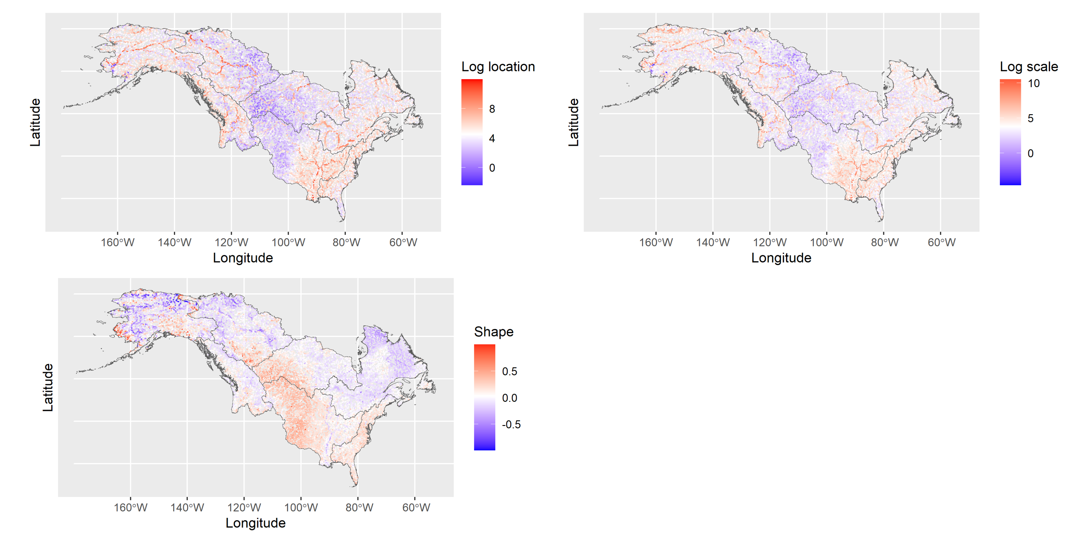
The predicted GEV distribution parameters (posterior distribution mean) are presented spatially for all catchments in regions 5 to 11 in Figure 8. The location and scale parameters have a similar spatial pattern, with higher values being concentrated over major river basins located in Northern territories, Alaska and the East coast of America. Areas between longitude 120°W and 100°W exhibit the lowest location and scale values. The spatial pattern is coherent and despite the BHM model being applied independently to each HydroBASINS region, there is no discontinuity in estimated values when crossing the region borders.
The shape parameter exhibits a distinct spatial pattern from the other two parameters. Regions with the highest values of shape are located in the Midwest area and along the American east coast. They correspond to mountainous terrains or arid deserts for the Midwest and hurricane-prone coastal areas for the East coast. Generally, the shape parameter values decrease with the latitude, except for some very local areas in Alaska. However, estimation of the shape in this region is most uncertain due to fewer gauged stations compared to other regions, so the few high estimates of shape parameter there need to be interpreted with caution. Some discontinuity seems to be noticeable on the right border of region 9 (British Columbia).
To assess the effect of incorporating daily discharge data when available to estimate the GEV distribution parameters, we perform a comparative study for region 9 where a BHM model without using daily data (M0) is adjusted and compared to our BHM model (M1). Estimates of GEV distribution parameters for stations where daily data is available are presented in Figure 9 for the two models. Differences in estimated values of the location and scale parameters are negligeable. These parameters are easy to estimate and incorporating daily data in the model does not modify their estimations (median relative difference of 0.2% and 1.5% for the location and scale respectively, when incorporating daily data). The comparison shows more difference for the shape parameter, which is harder to estimate accurately. Including daily data adds useful information which applies a correction to the estimated shape values in some cases. The induced median relative bias is negligeable (3.5%) but the median relative difference is significant (22%), when using additional peak-over-threshold discharge data for inference of the shape parameter.
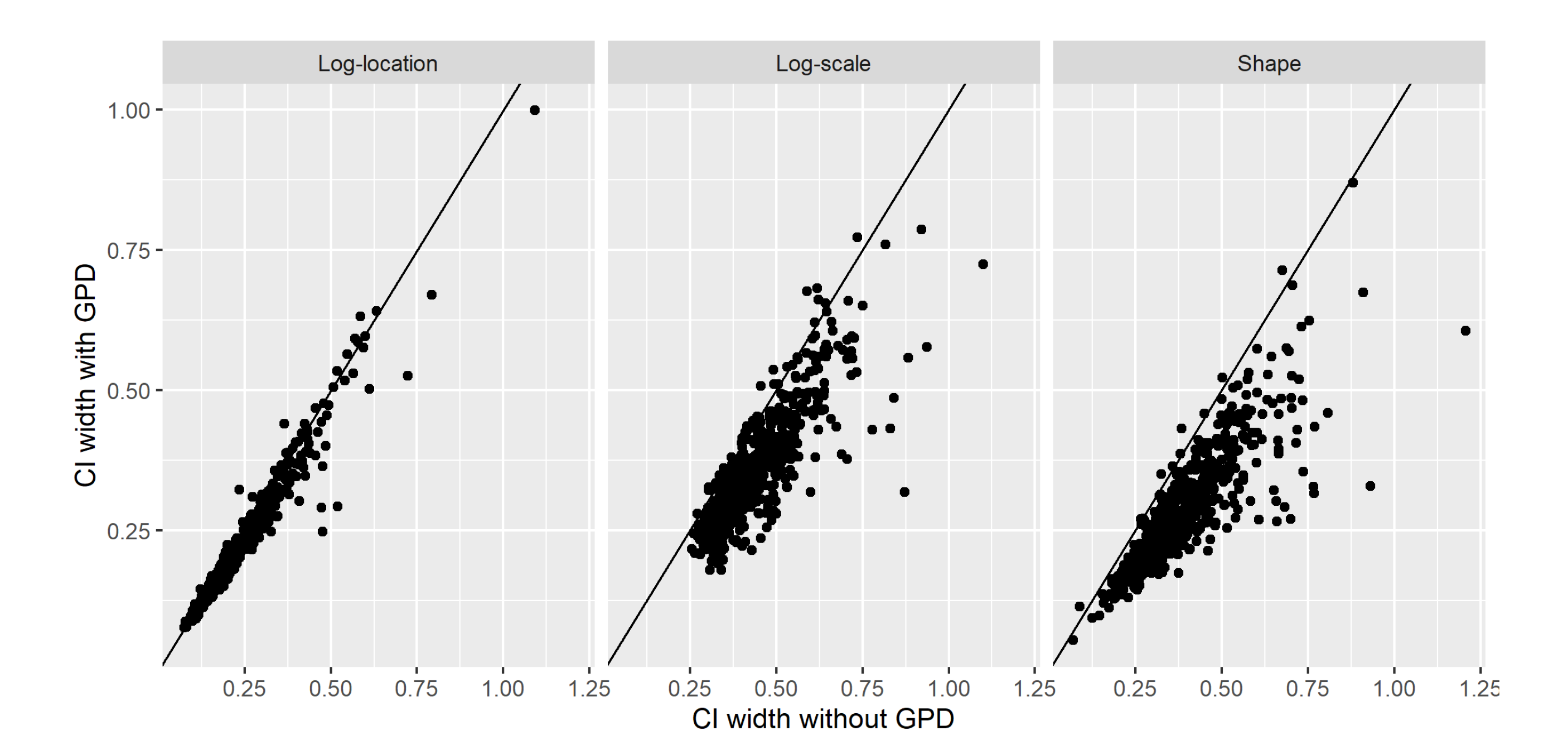
To further assess the added value of this approach, we compare the 95% confidence interval width of the GEV parameter distributions for the two models M0 and M1. Results are presented in Figure 10 for region 9. Reduction in uncertainty is present for all three parameters, particularly for the scale and shape parameters. The median relative reduction in the 95% confidence interval width is 6%, 18% and 26% for the log-location, log-scale and shape parameter respectively. This reduction in uncertainty is of significant impact as it propagates to the subsequent calculation of discharge extreme levels, which will be estimated with better precision for these stations. Finally, for stations where only annual maximum discharge data is available, we found no distinction in GEV distribution parameter estimates between models M0 and M1 (not shown).

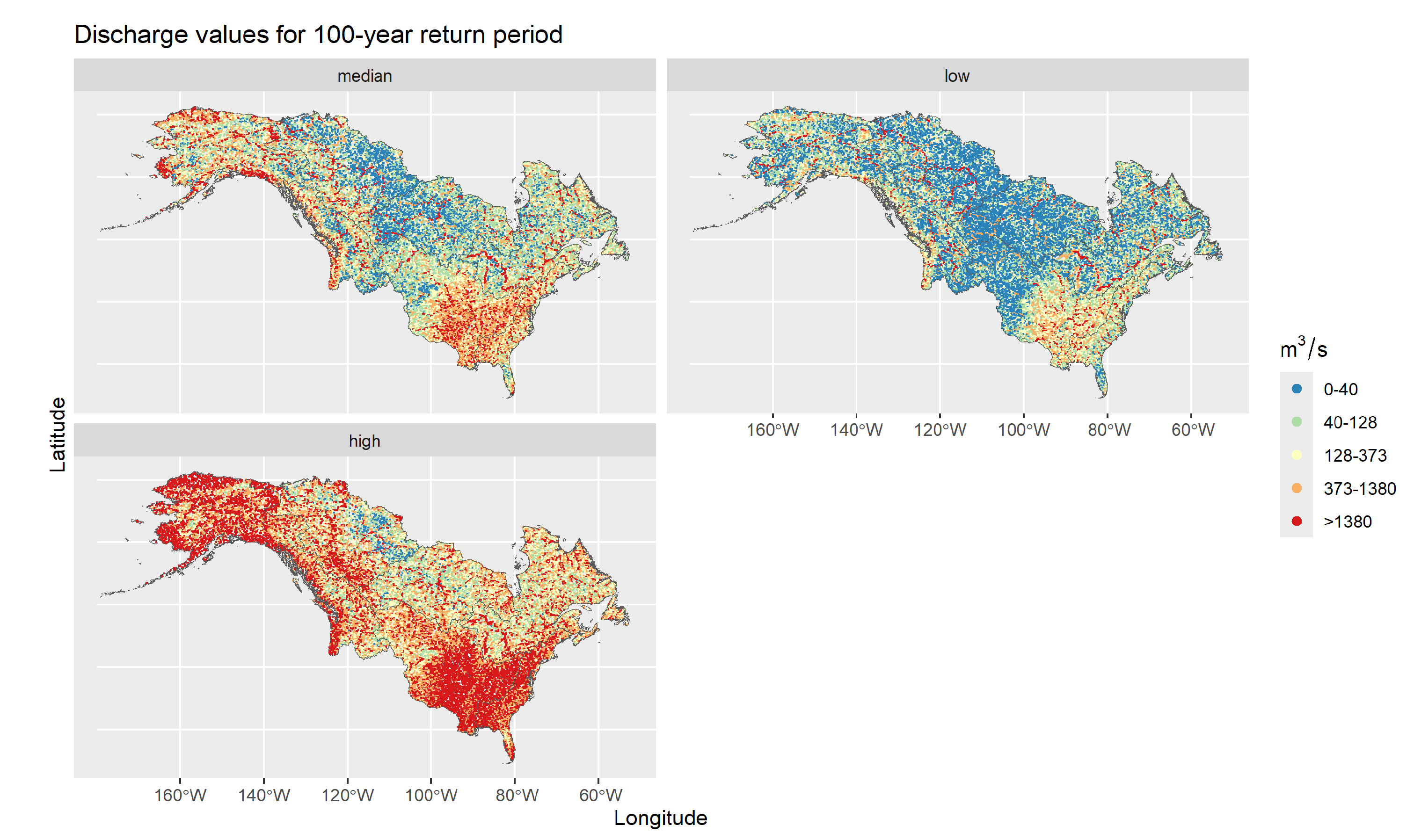
3.2.3. Peak Flow Return Levels

For the 100-year return period (RP100), corresponding discharge distribution median, 0.1th and 0.9th quantile values are plotted spatially for catchments in regions 5 to 11 in Figure 11. Higher discharge values are present in the north-west (Alaska and Northern territories) and south-east area (along the Mississippi river system and the American east coast). Continental areas in western US and central Canada exhibit lower RP100 discharge in general, as they more often correspond to river upstream, arid or mountainous areas. The spatial map of RP100 median discharge levels highlights the most prominent watercourses in North America: the Yukon river system in Alaska, the Mackenzie river in Northern Canada, the Mississippi river system in eastern USA and the Saint Lawrence basin in southern Quebec. The spatial maps of the 0.1th and 0.9th quantile for RP100 discharge levels show the high range of uncertainty when estimating extreme discharge levels, especially for higher return periods. As a matter of fact, the uncertainty from estimating the GEV distribution parameters is transferred to the return period peakflow, resulting in posterior predictive distributions for RP100 peak flows which are heavy-tailed.
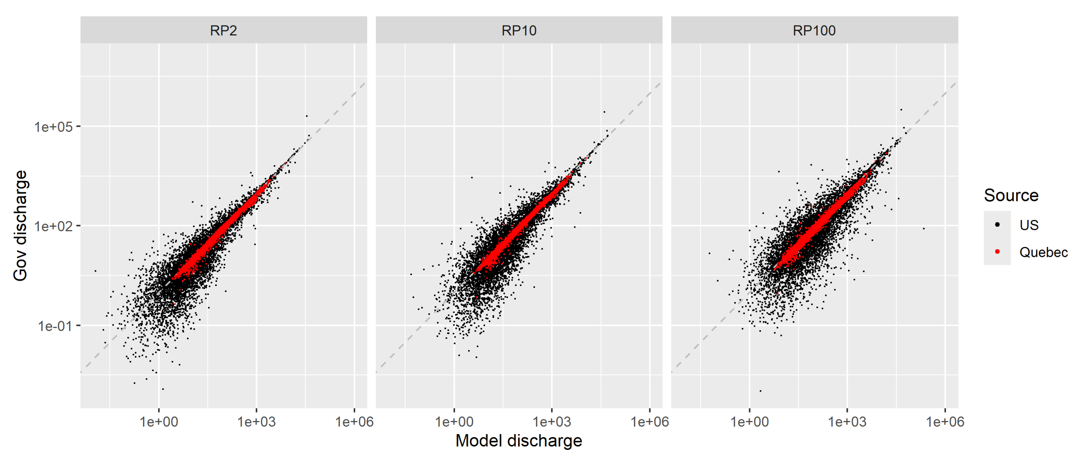
To further validate our extreme discharge estimates, we compare the 2, 10 and 100-year return period discharge values with corresponding return levels from two governmental sources: PeakFQ Program from USGS National Water data for the USA [29] and Ministère de l’Environnement et de la Lutte contre les changements climatiques for Quebec [32]. We did not find public return level data available for other areas in Canada. This comparison with governmental data is possible for around 21000 catchments in regions 5 to 11, with dense coverage over southern Quebec and all US territory except for Alaska. It is meant to verify the plausibility of our discharge estimates, though differences might arise due to different estimation methods. The US peakflows are calculated using the Log-Pearson type III distribution with several manual adjustments, while for Quebec, the best statistical distribution is used to fit well behaving stations locally, based on statistical criteria and graphical assessment. In Figure 12, discharge estimates for the 2, 10 and 100 year return periods from our model (x-axis) are compared with those from government sources (y-axis). There is a slight positive bias for small discharge values in our model compared to official estimates, but generally the overall bias is small. The spread of points indicate that our discharge estimates do not perfectly match the government estimates. Nevertheless, the reported median relative errors are 14.5 % for RP2, 14.5 % for RP10 and 18.6 % for RP100. The comparison is quite similar for the three return periods (low, medium and high extreme discharge values), indicating that differences from government sources arise from the bulk of the extreme discharge distributions rather than the tail. Interestingly, Figure 12 also shows that estimates from the Quebec government match our estimates much more closely than US data. Overall, the comparison shows satisfying agreement between our estimated peak flows and government-sourced peak flows.

4. Discussion and Conclusion

The spatial variations in flood extremes are modeled using 130 catchment specific covariates as described in Section 2.1.3. The fine spatial resolution of the catchment delineation used in our approach allows capturing complex local patterns in the GEV distribution parameters and return period peak flows. In the latent process layer of the Bayesian hierarchical model, we did not explicitly use a spatial structure as commonly found in the literature [12,20,23,44]. As explained in Section 3.1, the analysis of the regression residuals did not reveal any spatial patterns based on the Euclidean distance between the stations, suggesting that such dependencies are already accounted for by the 130 covariates. Secondly, implementing a spatial random field in the latent process would increase the computational complexity, which might be prohibitive when applied to a continental scale study. Finally, since the geographical extent is large, extensive work would be needed to choose the appropriate form of spatial structure and station distance metric to consider, which we consider outside of the scope of this study. Therefore, following the Occam’s razor principle, we adopted the more parsimonious model with random spatially independent regression errors in the latent process.
We saw that the shape parameter could not fully be described by our chosen set of covariates, as the regression errors remain substantial for the shape after fitting the BHM model. Estimating the shape parameter in regional flood frequency analysis is a notoriously complex problem [41,44], as this parameter is very sensitive to the data quality and length. Traditionally, to reduce uncertainty associated with its estimation, former models in the literature often assumed it to be constant across entire regions where RFFA is performed [12,15,22,45]. However, for the geographical extent used in our study, this simplistic assumption would be too restrictive because of hydrological spatial heterogeneity. As the geographical extent increases, patterns in climatology, terrain characteristics and hydrological behaviors which affect the flood regimes become more varied [46]. Therefore, we chose to model the shape parameter as a function of the static covariates at hand, which also allows prediction in ungauged catchments. Future areas of work can involve selecting more suitable covariates to improve the predictive power for the shape parameter. For example, [19] showed that for Norway, the ratio of snowmelt in the total precipitation is a strong predictor of the shape parameter. However, it is unclear whether such data is retrievable for North America and what would be their quality.
We chose to apply the model independently for each HydroBASINS level 2 region, where hydrological behaviors are assumed to be relatively similar, as opposed to having a unique unified model for the whole North America. Attempts to develop such a model showed a drop in model goodness-of-fit, which can be attributed to the heterogeneity of flood regimes and climatology across the continent. As a matter of fact, the Koppen-Geiger classification of climate zones in North America consists of 5-6 big climate zones, with marked variations depending on the latitude and elevation [47].
In this study, we developed a bayesian hierarchical model for regional flood frequency analysis at high spatial resolution in North America. Using our catchment delineation, flood peakflows can be estimated for every unit catchment with a mean area of 10 km 2 across the continent. We leverage approximately 20000 gauge station data and a rich dataset of 130 static covariates for 1.8 million catchments to build a predictive BHM and predict the GEV distribution parameters for ungauged catchments. Not only does our model account for statistical uncertainty in extreme peak flow estimates, it manages to reduce estimation uncertainty in cases where additional informative data is available. As a matter of fact, a novelty in our methodology consists in using both discharge annual maxima and excesses over a threshold in the data layer to estimate the GEV distribution parameters. This approach is able to reduce uncertainty at sites where both types of data are available, especially for the scale and shape parameters. The estimated discharge return levels are compared with official peakflows from government sources, showing satisfying agreement. An importance score is calculated to rank the 130 covariates, showing that the most significant indicators of peakflows are the catchment drainage area, the geographical location and temperature-based bio-indicators. Our study contributes to the overall push in the hydrological research community to improve RFFA flood estimates and provides application at the continental scale, paving the way for global scale flood risk analysis.

Supplementary Materials

The following supporting information can be downloaded at the website of this paper posted on Preprints.org.

Author Contributions

Conceptualization, D. Alexandre and C. Chaudhuri; methodology, D. Alexandre; software, D. Alexandre; validation, D. Alexandre and C. Chaudhuri; data curation, J. Gill-Fortin and C. Chaudhuri; writing—original draft preparation, D. Alexandre; writing—review and editing, C. Chaudhuri; visualization, D. Alexandre and J. Gill-Fortin; supervision, C. Chaudhuri. All authors have read and agreed to the published version of the manuscript.

Funding

This research was partly funded by the National Research Council of Canada Industrial Research Assistance Program.

Data Availability Statement

The gauge data used in the paper are available online in the GRDC database (https://portal.grdc.bafg.de/), on the USGS website (https://waterdata.usgs.gov/nwis/sw), on dedicated Canadian and Quebec platforms (https://collaboration.cmc.ec.gc.ca/cmc/hydrometrics/www/

Acknowledgments

We’d like to thank fellow Geosapiens team members Mingke Erin Li and Amit Kumar for their help with downloading and providing information on used datasets.

Conflicts of Interest

The authors declare no conflicts of interest.

References

  1. Centre for research on the epidemiology of disasters. The Human Cost of Natural Disasters - A global perspective, 2015.
  2. Kundzewicz, Z.W.; Kanae, S.; Seneviratne, S.I.; Handmer, J.; Nicholls, N.; Peduzzi, P.; Mechler, R.; Bouwer, L.M.; Arnell, N.; Mach, K.; Muir-Wood, R.; Brakenridge, G.R.; Kron, W.; Benito, G.; Honda, Y.; Takahashi, K.; Sherstyukov, B. Flood risk and climate change: global and regional perspectives. Hydrological Sciences Journal 2014, 59, 1–28. [Google Scholar] [CrossRef]
  3. Hirabayashi, Y.; Mahendran, R.; Koirala, S.; Konoshima, T.; Yamazaki, D.; Watanabe, S.; Kim, H.; Kanae, S. Global flood risk under climate change. Nature Climate Change 2013, 3, 816–821. [Google Scholar] [CrossRef]
  4. Engeland, K.; Hisdal, H.; Frigessi, A. Practical Extreme Value Modelling of Hydrological Floods and Droughts: A Case Study. Extremes 2004, 7, 5–30. [Google Scholar] [CrossRef]
  5. Nerantzaki, S.D.; Papalexiou, S.M. Assessing extremes in hydroclimatology: A review on probabilistic methods. Journal of Hydrology 2022, 605, 127302. [Google Scholar] [CrossRef]
  6. Katz, R.W.; Parlange, M.B.; Naveau, P. Statistics of extremes in hydrology. Advances in Water Resources 2002, 25, 1287–1304. [Google Scholar] [CrossRef]
  7. Coles, S.; Bawa, J.; Trenner, L.; Dorazio, P. An introduction to statistical modeling of extreme values; Vol. 208, Springer, 2001.
  8. Sivapalan, M.; Takeuchi, K.; Franks, S.; Gupta, V.; Karambiri, H.; Lakshmi, V.; Liang, X.; Mcdonnell, J.; Mendiondo, E.; O’Connell, P.; Oki, T.; Pomeroy, J.; Schertzer, D.; Uhlenbrook, S.; Zehe, E. IAHS decade on Predictions in Ungauged Basins (PUB), 2003-2012: Shaping an exciting future for the hydrological sciences. Hydrological Sciences Journal 2003, 48, 857–880. [Google Scholar] [CrossRef]
  9. Prihodko, L.; Denning, A.; Hanan, N.; Baker, I.; Davis, K. Sensitivity, uncertainty and time dependence of parameters in a complex land surface model. Agricultural and Forest Meteorology 2008, 148, 268–287. Chequamegon Ecosystem-Atmosphere Study Special Issue: Ecosystem-Atmosphere Carbon and Water Cycling in the Temperate Northern Forests of the Great Lakes Region. [CrossRef]
  10. Müller Schmied, H.; Adam, L.; Eisner, S.; Fink, G.; Flörke, M.; Kim, H.; Oki, T.; Portmann, F.T.; Reinecke, R.; Riedel, C.; Song, Q.; Zhang, J.; Döll, P. Variations of global and continental water balance components as impacted by climate forcing uncertainty and human water use. Hydrology and Earth System Sciences 2016, 20, 2877–2898. [Google Scholar] [CrossRef]
  11. Hosking, J.R.M.; Wallis, J.R. Regional Frequency Analysis: An Approach Based on L-Moments; Cambridge University Press, 1997. [CrossRef]
  12. Renard, B. A Bayesian hierarchical approach to regional frequency analysis. Water Resources Research 2011, 47. [Google Scholar] [CrossRef]
  13. Burn, D.H. Evaluation of regional flood frequency analysis with a region of influence approach. Water Resources Research 1990, 26, 2257–2265. [Google Scholar] [CrossRef]
  14. Gelman, A.; Carlin, J.B.; Stern, H.S.; Dunson, D.B.; Vehtari, A.; Rubin, D.B. Bayesian Data Analysis, 3rd ed.; Chapman and Hall/CRC, 2013. [CrossRef]
  15. Yan, H.; Moradkhani, H. A regional Bayesian hierarchical model for flood frequency analysis. Stochastic Environmental Research and Risk Assessment 2015, 29, 1019–1036. [Google Scholar] [CrossRef]
  16. Sampaio, J.; Costa, V. Bayesian regional flood frequency analysis with GEV hierarchical models under spatial dependency structures. Hydrological Sciences Journal 2021, 66, 422–433. [Google Scholar] [CrossRef]
  17. Lima, C.H.; Lall, U.; Troy, T.; Devineni, N. A hierarchical Bayesian GEV model for improving local and regional flood quantile estimates. Journal of Hydrology 2016, 541, 816–823. [Google Scholar] [CrossRef]
  18. Eastoe, E.F. Nonstationarity in peaks-over-threshold river flows: A regional random effects model. Environmetrics 2019, 30. [Google Scholar] [CrossRef]
  19. Thorarinsdottir, T.L.; Hellton, K.H.; Steinbakk, G.H.; Schlichting, L.; Engeland, K. Bayesian Regional Flood Frequency Analysis for Large Catchments. Water Resources Research 2018, 54, 6929–6947. [Google Scholar] [CrossRef]
  20. Sharkey, P.; Winter, H.C. A Bayesian spatial hierarchical model for extreme precipitation in Great Britain. Environmetrics 2019, 30, e2529. [Google Scholar] [CrossRef]
  21. Dyrrdal, A.V.; Lenkoski, A.; Thorarinsdottir, T.L.; Stordal, F. Bayesian hierarchical modeling of extreme hourly precipitation in Norway. Environmetrics 2015, 26, 89–106. [Google Scholar] [CrossRef]
  22. Wu, Y.; Xue, L.; Liu, Y. Local and regional flood frequency analysis based on hierarchical Bayesian model in Dongting Lake Basin, China. Water Science and Engineering 2019, 12, 253–262. [Google Scholar] [CrossRef]
  23. J. A. García, J. Martín, L.N.; Acero, F.J. A Bayesian hierarchical spatio-temporal model for extreme rainfall in Extremadura (Spain). Hydrological Sciences Journal 2018, 63, 878–894. [Google Scholar] [CrossRef]
  24. Kordrostami, S.; Alim, M.A.; Karim, F.; Rahman, A. Regional Flood Frequency Analysis Using an Artificial Neural Network Model. Geosciences 2020, 10. [Google Scholar] [CrossRef]
  25. Aziz, K.; Rahman, A.; Fang, G.; Shrestha, S. Application of artificial neural networks in regional flood frequency analysis: a case study for Australia. Stochastic Environmental Research and Risk Assessment 2014, 28, 541–554. [Google Scholar] [CrossRef]
  26. Zhao, G.; Bates, P.; Neal, J.; Pang, B. Design flood estimation for global river networks based on machine learning models. Hydrology and Earth System Sciences 2021, 25, 5981–5999. [Google Scholar] [CrossRef]
  27. Mangukiya, N.K.; Sharma, A. Alternate pathway for regional flood frequency analysis in data-sparse region. Journal of Hydrology 2024, 629, 130635. [Google Scholar] [CrossRef]
  28. Santillán, D.; Mediero, L.; Garrote, L. Modelling uncertainty of flood quantile estimations at ungauged sites by Bayesian networks. Journal of Hydroinformatics 2013, 16, 822–838. [Google Scholar] [CrossRef]
  29. U.S. Geological Survey. National Water Information System data available on the World Wide Web (USGS Water Data for the Nation), 2016.
  30. Environment and Climate Change Canada. HYDAT Database - Canada, 2013.
  31. Recknagel, T.; Färber, C.; Plessow, K.; Looser, U. The Global Runoff Data Centre: A building block in the chain of reproducible hydrology. EGU General Assembly 2023;, 2023. Abstract EGU23-15454.
  32. Ministère de l’Environnement, de la Lutte contre les changements climatiques, de la Faune et des Parcs. Atlas hydroclimatique, 2022.
  33. Lachance-Cloutier, S.; Turcotte, R.; Cyr, J.F. Combining streamflow observations and hydrologic simulations for the retrospective estimation of daily streamflow for ungauged rivers in southern Quebec (Canada). Journal of Hydrology 2017, 550, 294–306. [Google Scholar] [CrossRef]
  34. Lehner, B.; Grill, G. Global river hydrography and network routing: baseline data and new approaches to study the world’s large river systems. Hydrological Processes 2013, 27, 2171–2186. [Google Scholar] [CrossRef]
  35. Yamazaki, D.; Ikeshima, D.; Sosa, J.; Bates, P.D.; Allen, G.H.; Pavelsky, T.M. MERIT Hydro: A High-Resolution Global Hydrography Map Based on Latest Topography Dataset. Water Resources Research 2019, 55, 5053–5073. [Google Scholar] [CrossRef]
  36. Arc Hydro Team. Arc Hydro Toolbox 2.8.17, 2021.
  37. Robert, C.P.; Casella, G. Monte Carlo Statistical Methods, 2nd ed.; Springer Science & Business Media: New York, NY, 2004. [Google Scholar]
  38. Roberts, G.O.; Rosenthal, J.S. Examples of Adaptive MCMC. Journal of Computational and Graphical Statistics 2009, 18, 349–367. [Google Scholar] [CrossRef]
  39. Roberts, G.O.; Rosenthal, J.S. Optimal scaling for various Metropolis-Hastings algorithms. Statistical Science 2001, 16, 351–367. [Google Scholar] [CrossRef]
  40. Love, C.A.; Skahill, B.E.; England, J.F.; Karlovits, G.; Duren, A.; AghaKouchak, A. Integrating Climatic and Physical Information in a Bayesian Hierarchical Model of Extreme Daily Precipitation. Water 2020, 12. [Google Scholar] [CrossRef]
  41. Sang, H.; Gelfand, A.E. Hierarchical modeling for extreme values observed over space and time. Environmental and Ecological Statistics 2009, 16, 407–426. [Google Scholar] [CrossRef]
  42. Morrison, J.E.; Smith, J.A. Stochastic modeling of flood peaks using the generalized extreme value distribution. Water Resources Research 2002, 38, 41–1. [Google Scholar] [CrossRef]
  43. Katz, R.W. Statistics of extremes in climate change. Climatic Change 2010, 100, 71–76. [Google Scholar] [CrossRef]
  44. Davison, A.C.; Padoan, S.A.; Ribatet, M. Statistical Modeling of Spatial Extremes. Statistical Science 2012, 27, 161–186. [Google Scholar] [CrossRef]
  45. Daniel Cooley, D.N.; Naveau, P. Bayesian Spatial Modeling of Extreme Precipitation Return Levels. Journal of the American Statistical Association 2007, 102, 824–840. [Google Scholar] [CrossRef]
  46. Michaud, J.D.; Hirschboeck, K.K.; Winchell, M. Regional variations in small-basin floods in the United States. Water Resources Research 2001, 37, 1405–1416. [Google Scholar] [CrossRef]
  47. Beck, H.E.; Zimmermann, N.E.; McVicar, T.R.; Vergopolan, N.; Berg, A.; Wood, E.F. Present and future Köppen-Geiger climate classification maps at 1-km resolution. Scientific Data 2018, 5, 180214. [Google Scholar] [CrossRef]
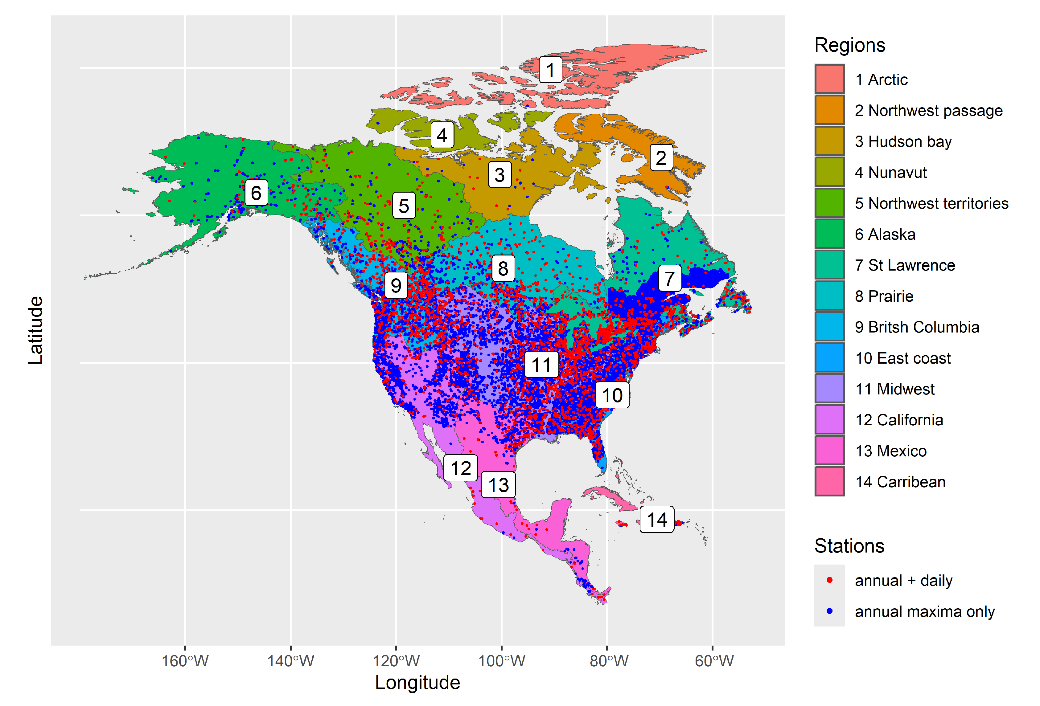
Figure 1. Station coverage and the 14 HydroBASINS level 2 regions for North America. Stations with only annual maximum data available are shown in blue, while stations with both types of data available are shown in red.
Preprints 111602 g001
Figure 2. Discretization of the HydroBASIN region 9 into river networks (left) and catchments, for a small river network (right). The considered network is highlighted with a red contour.
Preprints 111602 g002
Figure 3. Bayesian hierarchical model structure.
Preprints 111602 g003
Figure 4. BHM model validation for regions 5 to 11, using a hold-out validation procedure. For validation sites, GEV distribution parameter estimated with the BHM model (x axis) are compared with their local estimates (y axis). The Pearson correlations for this comparison are also reported. A random half of the data is used for training and the other half for validation.
Preprints 111602 g004
Figure 5. Normal quantile quantile plots for the three GEV distribution parameter residuals for all gauged data, regions 5 to 11.
Preprints 111602 g005
Figure 6. Spatial representation of the regression residuals, for the three GEV distribution parameters and for all gauged stations in regions 5 to 11. The residuals are classified into 4 groups splitted by the first, second and third quartile.
Preprints 111602 g006
Figure 7. The top ten most significant covariates to predict GEV distribution parameters with the BHM model. The y-axis shows the covariate nomenclatures while the x-axis shows the importance score. The score is defined by summing the absolute value of the corresponding regression coefficients across all regions, after regional standardization and elimination of non-significant covariates.
Preprints 111602 g007
Figure 8. GEV distribution parameter estimates (mean of posterior distributions) for catchments in regions 5 to 11. Red, white and blue correspond to high, medium and low values respectively
Preprints 111602 g008
Figure 9. Comparison of GEV distribution parameter median estimates for the BHM model without daily data (x axis) and our BHM model with additional daily data (y axis). The comparison is done for all stations in region 9 where daily discharge data is available.
Preprints 111602 g009
Figure 10. Comparison of GEV distribution parameter 95% confidence interval width for the BHM model without daily data (x axis) and our BHM model (with additional daily data). The comparison is done for all stations in region 9 where daily discharge data is available.
Preprints 111602 g010
Figure 11. The 100 year return period discharge levels are plotted for catchments in regions 5 to 11. The three plots correspond to the median, lower end (0.1th quantile) and upper end (0.9th quantile) of the RP100 discharge distribution.
Preprints 111602 g011
Figure 12. Comparison of BHM model estimated discharge with those from government sources (black and red dots for the US and Quebec respectively), for the 2, 10 and 100 year return periods, for regions 5 to 11.
Preprints 111602 g012
Disclaimer/Publisher’s Note: The statements, opinions and data contained in all publications are solely those of the individual author(s) and contributor(s) and not of MDPI and/or the editor(s). MDPI and/or the editor(s) disclaim responsibility for any injury to people or property resulting from any ideas, methods, instructions or products referred to in the content.
Copyright: This open access article is published under a Creative Commons CC BY 4.0 license, which permit the free download, distribution, and reuse, provided that the author and preprint are cited in any reuse.
Prerpints.org logo

Preprints.org is a free preprint server supported by MDPI in Basel, Switzerland.

Subscribe

© 2024 MDPI (Basel, Switzerland) unless otherwise stated