
Submitted:
08 July 2024
Posted:
10 July 2024
You are already at the latest version
Abstract
The StarDICE experiment strives to establish an instrumental metrology chain with a targeted accuracy of 1 mmag in griz bandpasses to meet the calibration requirements of next-generation cosmological surveys. Atmospheric transmission stands out as a significant source of systematic uncertainty. Specifically, gray extinction induces spurious variations of photometric fluxes. We propose a solution relying on an uncooled long-wave infrared thermal camera to evaluate it. This type of camera can provide real-time insights into atmospheric conditions and detect cirrus clouds. However, achieving accurate measurements with thermal imaging systems necessitates prior calibration due to the influence of temperature-induced effects, which compromise their spatial and temporal precision. Moreover, these systems cannot provide scene radiance values in physical units by default. This study introduces a new calibration process utilizing a tailored forward modeling approach. The method is applied to an uncooled FLIR Tau2 thermal camera. It incorporates sensor, housing, flat-field support, and ambient temperatures, along with raw digital response, as input data. Experimental measurements are conducted inside a climatic chamber, with the camera imaging a thermoregulated blackbody source. Results demonstrate the calibration effectiveness, achieving precise radiance measurements with a temporal pixel root-mean-square error (RMSE) of 0.09 W/m2/srand residual spatial noise of 0.03 W/m2/sr.
Keywords:
uncooled infrared thermal camera calibration
; cirrus cloud
; atmosphere monitoring
; gray extinction
; low radiances
1. Introduction
Ground-based astronomical surveys like PanSTARRS [1], the Dark Energy Survey [2], and the Vera Rubin Observatory Legacy Survey of Space and Time (LSST) [3] demand precise broadband photometry [4]. The LSST Dark Energy Science Collaboration requires achieving 5 milli-magnitudes (mmag) and 1 mmag precision in filters for first and 10-year type 1a supernovae (SNe Ia) analyses respectively [5]. Meeting this standard is crucial for deriving competitive cosmological insights from SNe Ia data.
In that respect, the StarDICE [6] metrology experiment has emerged with the intended purpose of measuring and comparing the brightness of stars from the CALSPEC library of spectrophotometric standards [7] against laboratory flux references, represented by photodiodes calibrated by the National Institute of Standards and Technology (NIST) [8]. The improved standards catalog provided by StarDICE will serve as the foundation for propagating calibration to stellar sources that are or will be observed by telescopes such as the Simonyi Survey Telescope of the Vera C. Rubin Observatory [9]. The StarDICE pathfinder project [10] has determined that the last major source of systematic uncertainty exceeding the mmag threshold is caused by the atmosphere. Directly measuring and correcting for atmospheric transmission variations will be necessary to significantly enhance the precision of the observations. Specifically, thin high-altitude cirrus clouds can induce spurious variations known as gray extinction [11,12]. They are challenging to detect but it is essential to properly characterize them to extract above atmosphere reference star fluxes.
In the context of this astronomical calibration experiment, we explore a possible solution relying on an uncooled infrared thermal camera (UIRTC) to evaluate astronomical observation quality with respect to gray extinction contamination.
The utilization of IR thermal cameras has emerged as a useful source of information for atmospheric investigations through precise radiometric measurements [13,14,15,16,17,18]. Prior research has demonstrated these sensors’ ability to provide high-speed, compact, and cost-effective means to characterize atmospheric conditions by imaging the sky downwelling radiance in the long-wave infrared (LWIR) range from 8 to 14 µm, centered around the atmosphere transparency window in the 10-12 µm range [19,20]. In this spectral region, after accounting for the effect of water vapor, the contrast between cloud radiance and clear sky background radiance is relatively high, exceeding a difference of 0.1 [19]. Previous work established the feasibility of using UIRTCs to obtain reliable radiometric atmosphere measurements for astronomy-related applications [21,22]. Klebe et al. [17] already observed the direct sky’s thermal radiance by developing an all-sky IR thermal camera instrument. They successfully determined the sky cover fraction and estimated the precipitable water vapor (PWV), which impacts near-IR photometry. Hack et al. [23] advanced this work by comparing measurements and simulations of sky downwelling radiance. Under stable atmospheric conditions, they achieved PWV determination with an accuracy of approximately 2%. This required an instrument that had undergone prior radiometric calibration.
For conventional cooled thermal cameras, the radiometric calibration model is formulated by building the relation between image pixel values and corresponding blackbody temperatures in a controlled laboratory setting [24]. This model is presumed to be long-term effective in real-world applications as the camera will operate at the same stabilized temperature. This assumption is unsuitable for uncooled thermal cameras for which temporal and spatial non-uniformities prevail on images, leading to substantial errors in radiance retrieval when the camera operates in unstable conditions, such as varying ambient temperatures [14,19,25]. Therefore, the use of UIRTCs presents challenges that must be overcome before they can be used for atmosphere monitoring purposes as Ribeiro-Gomes et al. [26] pointed out, including: (i) spatial non-uniformity; (ii) ambient and sensor temperature drift while the object’s temperature remains constant, due to uncompensated focal plane array (FPA) temperature variations; (iii) FPA-temperature-dependent response; (iv) fixed pattern noise (FPN).
To address the aforementioned challenges, the work presented here introduces a shutter-based radiometric calibration method designed specifically for UIRTCs and optimized for low-temperature measurements. Our method relies on a model that integrates camera housing, FPA, flat-field support and ambient temperature variations, rendering it suitable for instruments operating in less stable environmental conditions. This approach mitigates signal perturbations arising from fluctuations in ambient temperature and internal heating of the camera. We also developed a forward model to estimate the total scene radiance in .
The paper is structured as follows. Section 2.1 provides the rationale for this study, discussing the current state-of-the-art calibration methods. Section 2.2 describes the experimental setup. The real-time non-uniformity correction (NUC) procedure is detailed in Section 2.3. Section 2.4 introduces the scene radiance model, while Section 2.5 focuses on its specific features for laboratory measurements. The complete radiometric calibration model is presented in Section 2.7. Section 2.8 details the data acquisition procedure and dataset. The data fitting method using the least-squares algorithm is explained in Section 2.9. Section 3.1 presents the results of the improved flat-field correction method. The calibration results are analyzed in Section 3.2 and Section 3.3. Section 3.4 demonstrates the application of the calibration method to a real case study and compares radiometric images to radiative transfer simulations. Section 4 examines potential limitations of the calibration procedure and suggests revisions. Finally, Section 5 summarizes the main findings and outlines future work.
2. Materials and Methods
Our goal for calibrating a UIRTC centers on attaining precise characterization of atmospheric gray extinction, with a specific emphasis on measuring the low radiance of the sky. It comprises an experimental setup ensuring controlled conditions, a systematic data acquisition process, and a novel calibration model for enhanced radiometric measurements. An improved in-situ non-uniformity correction mitigates potential artifacts. Performance metrics and data fitting processes validate the calibration model’s efficiency. This concise and integrated approach ensures precise thermal products suitable for atmospheric gray extinction studies.
2.1. Motivation
The primary objective of the calibration experiment is to correct raw observations for defects and to convert the analog-to-digital units (ADUs) read from the camera to the emitted sky radiance , establishing a relationship with true physical radiances. Once true radiance images of the sky are obtained, cloud structures can be extracted. The conceptual principles of the calibration process are the following. Images of a blackbody emitter at multiple temperatures are taken with the camera placed in a temperature-controlled environment. A pixel response model is fitted on these images to produce calibration matrices that will be used a posteriori to calibrate in-field images. The flowchart shown in Figure 1 summarizes this process.
Many methods have been proposed and implemented to address this issue, specifically to correct for the different noise sources mentioned above. For a concise overview and state-of-the-art comparisons, we refer the reader to the work of González-Chávez et al. [27]. Several approaches focus on shutterless calibration methods, as relying on the shutter for flat-field support leads to interruptions and a reduction in the maximum frame rate of the cameras. In our specific use case, the flat-field-based method does not impact our research, as we leverage the overhead between CCD optical exposures (i.e., while the filter wheel is rotating or when reading the previous image). The majority of methods focus solely on temperature measurements, utilizing the temperature of the calibration blackbody source as a reference. The process typically involves a two-step approach: (i) correcting for sensor temperature drift and camera self-emission on raw digital images; (ii) performing temperature radiometric calibration by associating corrected ADUs with blackbody temperature setpoints. However, these methods rely on assumptions that are effective only under specific conditions. Notably, when working with low blackbody source temperatures (i.e., sub-zero degrees Celsius), considerations for the emissivity of the blackbody source and ambient contributions become crucial for accurately evaluating the observed radiance perceived by the camera. To correct ADUs, most techniques first assumed that the ambient contribution to the scene radiance is consistent across all camera and blackbody temperature setpoints. Images are then normalized to the user-defined reference level to stabilize the image signal. Nonetheless, in practice, temperature changes in the climate chamber housing the camera (especially when near the calibration blackbody) can cause the camera to perceive radiance originating partially from the chamber itself. The colder the blackbody source temperature, the higher the ambient scene contribution to the total scene radiance.
In this study, we undertake a different approach by developing a radiance calibration model that accounts for this effect and apply it to our dataset, adding ambient thermal emission to the blackbody source in the observed scene radiance.
2.2. Experimental Setup
The experimental calibration setup is depicted in Figure 2 and a simplified sketch is shown in Figure 3. The thermal camera is positioned within a climatic chamber, serving as an environmental enclosure to replicate ambient temperatures akin to those that will be experienced during in-situ measurements at Observatoire de Haute-Provence to monitor the cloud coverage. It receives homogeneous and isotropic thermal emission from the blackbody source located at a specific fixed distance to cover the entire field-of-view (FOV) of the camera.
The thermal camera used for this experiment is the FLIR Tau2 (FLIR Systems Inc., Wilsonville, OR, USA) operating in the LWIR range (8-14 µm). It is coupled to a Umicore athermalized 60 mm f#1.251 lens, which provides a scale of 1 arcmin/pixel. The sensor is an array of 640 × 512 vanadium oxide (VOx) pixels of 17 µm square size. Figure 4 depicts the camera’s throughput as a function of wavelength, as given by the manufacturer for a typical Tau2 core model. The announced operational scene temperature range in high-gain mode is -40 °C to +160 °C. In radiometric mode, the incident radiance is digitized over 14-bit depth at a high frame rate of 8.33 Hz provided by the ThermalGrabber USB 2.0 interface from TeAx. Two temperature sensors are implemented inside the camera. One is located on the FPA next to the microbolometers array and provides temperatures with 0.1 °C resolution. The other is built-in inside the camera’s housing (closer to the outer walls of the case) and has a resolution of 0.01 °C.
The manufacturer announces a Noise Equivalent Temperature Difference (NETD) of 50 mK for a f#1.0 lens at = 300 K target temperature with unit emissivity2. This figure of merit defines the minimum temperature difference that can be detected with a signal-to-noise ratio (SNR) of 1. Transforming this sensitivity value into the Noise Equivalent Radiance Difference (NERD) for this specific camera lens combination requires the following calculation,
with the Planck function and the instrument throughput shown in Figure 4. For this camera and target temperature of 300 K, the NERD equivalent to the NETD of 50 mK is equal to 0.044 . Figure 5 plots the NERD as a function of target temperature (blue scale) and equivalent scene radiance (red scale). The plotted curves can be interpreted as a lower boundary spatial noise limit per image.
The blackbody calibrator source is the IR-2101/301 model from Infrared Systems Development. This source provides a 63.5 × 63.5 mm2 emitting surface area with temperatures ranging from -30 °C to +80 °C. The blackbody emissivity is equal to , with ± 0.1 °C temperature monitoring sensor resolution calibrated with ± 0.2 °C uncertainty level relative to a NIST standard3. Operation of the blackbody is done through a standard RS-232 serial port. Blackbody temperatures used in the calibration process ranged from -30°C to 60°C, which covers the linear range of the camera response down to the lowest achievable temperature in the experimental setup conditions.
For the external flat-field support, we use a thin 2 mm copper plate placed at ∼ 5 cm distance from the camera, facing the lens and covered with high-emissivity 3M Scotch Super 88 Vinyl electrical tape. Benirschke and Howard [28] and Avdelidis and Moropoulou [29] used this tape, whose emissivity is at °C. FLIR also recommends using this electrical tape and states that it has an emissivity of 0.96 in the long wavelength (8-12 µm) range4. The plate is attached to a high-torque servomotor which rotates it in front of the camera lens. A Raspberry Pi controls the servomotor movement through pulse with modulation (PWM) signals. The in-situ shutter-based type correction is performed at regular intervals of 30 seconds. It consists in positioning the flat-field support in front of the camera lens and activating the non-uniformity correction (NUC, equivalent to FFC) with the camera control-command software. The flat-field support surface is monitored by a temperature sensor. One measurement is sampled just before starting the NUC procedure and given to the camera microcontroller as required for internal computation [30,31].
Every instrument, including the camera, the blackbody source, the external flat-field system, and temperature sensors were positioned inside a climatic chamber. It consists of an insulated facility equipped with heating and cooling systems, as well as control electronics, that is used to create a stable and repeatable environment. We use the Weisstechnik LabEvent L T/150/70/3 climatic chamber at IJCLab in Orsay. Relative humidity was kept below 2%, which was required to cool the blackbody source down to -30 °C without producing frost on the surface. The aperture window of the climatic chamber was covered with several layers of aluminum foils to prevent exterior stray light from disrupting the measurements.
2.3. Improved In-Situ Non-Uniformity Correction
Non-uniformity correction (NUC) is essential for mitigating pixel-to-pixel sensitivity variations in thermal cameras, primarily caused by differences in the microbolometers characteristics [32]. The most common approach, known as the shutter-based flat field correction (FFC) method, relies on capturing periodic images with a closed shutter [30,31]. This process allows for precise adjustments to the pixel offsets, effectively reducing fixed-pattern noise (FPN) and ensuring the generation of accurate and uniform images. Generally, the most used FFC method triggers a NUC at regular intervals or with a temperature change and often falls short of achieving optimal correction. While suitable for applications with less stringent accuracy requirements, it has limitations regarding vignetting correction due to optics placed in front of the shutter. One solution, proposed by Budzier and Gerlach [33] involves fine-tuning of the camera firmware to process and save FFC frames for post-processing. Implementing such methods is challenging due to limited access and knowledge of the embedded software governed by the manufacturer’s discretion.
Two patents have been filed by the camera manufacturer which describe the method operating internally [30,31]. In short, multiple images of the FFC support are averaged, the FPA temperature is read and some pixel-to-pixel scaling map is computed with pre-configured tables stored in the camera firmware.
One alternative approach available to improve the process involves activating the camera’s external NUC mode. While this method employs the default correction algorithm, it uses an emitting surface positioned in front of the camera optics.
As the user can provide any type of surface in front of the lens during the FFC operation, using a homogeneous high emissivity support can improve the correction compared to the internal shutter. In particular, it will remove any emission or vignetting due to the lens. This workaround provides a viable option when extensive modifications to the camera’s firmware are not feasible.
2.4. Generic Scene Radiance Model
The scene radiance observed by a detector in the general case is presented in Figure 6. The radiance perceived by the camera FPA is the sum of scene radiance passing through the atmosphere (red arrow), the reflected background radiance onto the scene passing through the atmosphere (blue arrow), the atmospheric radiance, and the ambient radiance surrounding the camera (gray arrow). This ambient radiance (green arrow) is the direct emission of the environment surrounding the camera. The contributions to the scene radiance can be summarized in the following equation,
where is the sum of spectral radiances () arriving at the detector, is the wavelength, is the atmosphere transmission coefficient, the object emissivity, , , and are the radiances emitted by the object, the background surrounding the scene reflected by the object, the ambient environment surrounding the camera, and the atmosphere respectively. We assume that the object reflection coefficient is .
UIRTCs measure the integral of the spectral radiance emitted by the scene within the sensor spectral band limits and throughput ,
with the scene radiance observed by the instrument in . is the combination of optics and sensor throughputs (see Figure 4).
2.5. Close-Up Views Radiance Model
For close-up views, such as laboratory measurements, atmospheric emission, and transmission do not affect the flux as optical thickness is negligible, and = 0. It is necessary to keep the ambient radiance component for reasons explained in Section 2.7. Equation 2 simplifies to the following expression for our laboratory measurements,
A commonly employed calibration radiation source is a blackbody emitter source with temperature regulation that has a homogeneous and isotropic emission surface with high emissivity [34]. Strictly speaking, this is a grey body with a uniform emissivity close to 1. The radiance emitted by this blackbody at temperature and captured by the UIRTC can be calculated using the standard Planck formula :
where represents the radiance integrated in the bandpass of the instrument, is the blackbody emissivity, is the spectral radiance of a blackbody radiator at temperature . h is the Planck constant, c is the speed of light and is the Boltzmann constant. Lastly, the integrated radiance observed by the camera during calibration is,
with the background emission at ambient temperature of the climatic chamber and the blackbody radiance is the object radiance from Equation 4. The background radiance contribution is a reflection of the ambient radiance onto the blackbody surface filling the camera’s FOV.
2.6. Thermal Interactions Inside the Camera
The lower panel of Figure 6 focuses on the heat exchanges inside the camera and derives from the model of Tempelhahn et al. [35]. is the radiance of the scene entering the camera in the projected solid angle (orange). is the camera housing emission within the solid angle (purple). is the pixel self-emission into the half-space projected solid angle (cyan). Tempelhahn et al. [35] proposed an expression for the net radiant flux on the pixel (i,j) with the corresponding projected solid angles and respectively,
where is the pixel surface area, is the scene radiance defined in Equation 6, and are the camera housing emission (computed by integrating the Planck function with camera temperature ) towards the microbolometers and the pixel self-emission integrated over the sensor throughput. The emissivity of the microbolometers is assumed to be . Tempelhahn et al. [36] have shown that the pixel’s FOV covers nearly the entire half space for this kind of infrared thermal camera. Therefore, the corresponding pixel’s projected solid angle amounts almost to and is constant for all pixels independent of their position. The projected solid angle depends on the optics focal ratio: for the lens mounted on our camera with f# = 1.25. The remaining projected solid angle . The projected solid angles and of each pixel (i,j) depend on the position within the FPA and are symmetrically distributed around the optical axis of the IR optics.
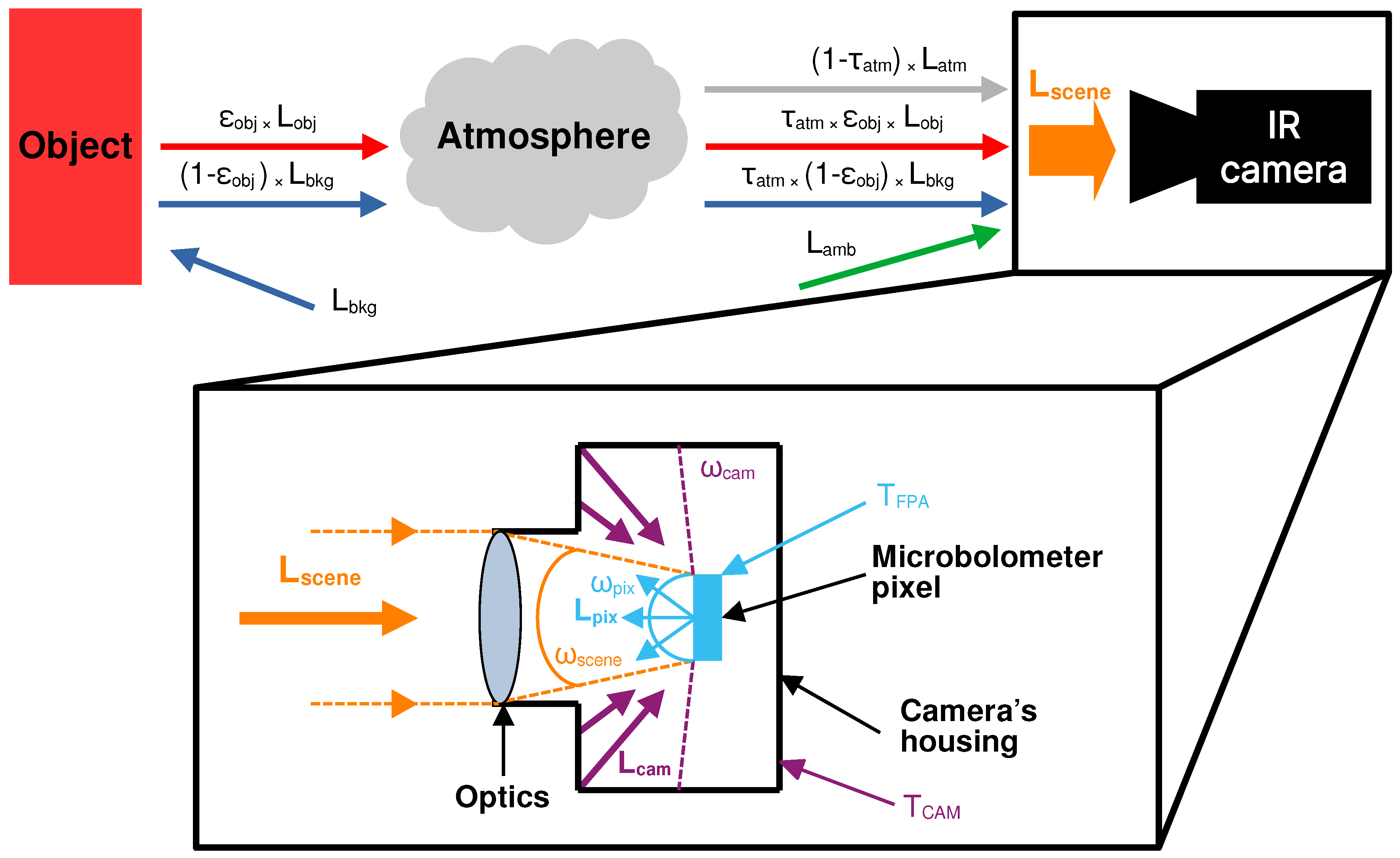
Figure 6.
Schematic of radiance contributions for radiometric measurements. The upper panel details the contribution from the outside environment, whereas the lower panel illustrates radiative transfers occurring inside the camera.
Figure 6.
Schematic of radiance contributions for radiometric measurements. The upper panel details the contribution from the outside environment, whereas the lower panel illustrates radiative transfers occurring inside the camera.
2.7. Calibration Model
The radiant net flux on each pixel (i,j) induces the temperature increase of the microbolometer. The voltage V read by the analog-to-digital converter (ADC) and converted to analog-to-digital units (ADUs) S is proportional to the thermal resistance variation of the microbolometer [37]. In the range of temperatures considered, we assume that the resistance and temperature variations are linearly related. We discuss about the non-linearity in Section 4.3. In our baseline model we express linearly the raw response as a function of the net flux,
where is the camera raw response of the (i, j) pixel expressed in ADUs, is the sensor responsivity in and is the offset signal in ADU. Note that the gain and offset parameters are given for a unique pixel, corresponding to a unique microbolometer, as a consequence of non-uniformity of the responses caused by optical relative irradiance, housing straylight, and detector pixel-to-pixel differences due to manufacturing process [38].
By injecting the radiant flux expression from Equation 7 into Equation 8, we can separate the scene radiance from other contributions,
The pixel gain is expressed as,
The individual offsets are
where represent the offset from Equation 8, represents the camera housing emission and the microbolometer outward self-emission with the temperature of the focal plane array. closely follows the evolution of due to heat propagation and equalization processes [35], except for some instants. Therefore, it is difficult to separate the effect of the camera housing emission from the pixel self-emission . The sensor temperature , is provided by the camera itself, and it is assumed that any variations are uniformly distributed across the entire sensor array. In contrast, the housing temperature sensor is placed at an unknown location inside the camera core and the associated thermal effects are not uniform.
We found that the residuals up to - 0.6 were correlated with the temperature difference (see Figure 7). By including an additional term for the difference - with the nuisance parameter , the residuals are reduced as shown in Figure 7. and are computed by integrating the Planck function over the total instrument throughput with the ambient temperature at each image instant and at the FFC time. This is due to diffuse radiation entering the camera through the lens. When doing an external FFC the camera is fed with the temperature of the external shutter at this specific time. However, this does not take into account ambient radiation from outside the FOV reaching the front lens of the camera and diffusing inside the housing. If the temperature of the environment changes after the FFC, this contribution is modified and affects the true scene radiance received by the FPA.
The complete calibration model is written
The vector of parameters to be adjusted for each pixel by the regression algorithm is .
The temperature dependence correction and the radiometric calibration are performed simultaneously. The two-step procedure, first compensating the raw signal for ambient temperature changes and then transforming the corrected ADU into temperature or radiance physical units, is not feasible with our setup. The main reason is that our experimental setup did not allow to maintain a fixed scene radiance while changing the environment and camera temperature. The environment radiance impacts the scene radiance as the blackbody source emissivity of 0.96 is not unity.
Figure 8 shows (computation using Equation 6) the relative difference of scene radiance caused by the ambient radiance reflected onto the blackbody source surface between a blackbody of emissivity = 1 and a blackbody with = 0.96. Unless the blackbody temperature matches the ambient temperature, the pixel ADU level contains a signal caused by the environment. This limits the achievable accuracy of our calibration experiment (see Section 4).
2.8. Acquisition Procedure and Dataset
The camera acquires images of a constant blackbody source radiance continuously while the climatic chamber (ambient temperature) is heated across a range of predefined temperatures of -5 °C, 0 °C, +5 °C, +10 °C and +15 °C. The frame acquisition rate was set at half the camera’s capacity, that is approximately 4 images per second. To probe ambient and flat-field support temperatures, we use two Sensirion STS-35-DIS temperature sensors with an accuracy of ± 0.1 °C for the +20 to +60 °C range and ± 0.2 °C for the -40 °C to +20 °C range. Data is transferred to the Raspberry Pi board through general-purpose input/output pins. The goal is to emulate imaging operation conditions at Observatoire de Haute-Provence where the camera will be installed with the StarDICE instrumentation. Due to time and hardware constraints, including lower or higher temperatures with more setpoints was not feasible. It was not possible to reach blackbody temperatures lower than -30°C with ambient temperatures above 15°C as the relative humidity level was too high to avoid water condensation on the device which could cause malfunction or permanent damage. Each image sequence is repeated for blackbody source temperature setpoints of -30°C, -20°C and -10°C.
IR images in raw 14-bit format are saved as FITS files containing temperature logs in metadata headers for post-processing (e.g., FPA temperature readings, flat-field support surface temperature, ambient temperature, blackbody temperature). To ease the control command of the camera and other equipment (see Figure 3), we developed multiple Python programs5,6.
Finally, to obtain more accurate temperature readings (e.g., FPA temperature, ambient temperature, camera housing temperature), readings were linearly interpolated for each image (taken at 9 Hz) as original measurements were sampled at 30-second intervals.
2.9. Data Fitting
The approach hinges on a forward modeling technique for the estimation of the scene radiance. Indeed, we do not have a direct measurement of the true radiance measured by the camera. The forward model computes the scene radiance observed by the instrument given by Equation 6, using , and parameters. Then, the vector of the calibration model parameters of defined in Equation 14 is adjusted onto this scene radiance. These parameters are fitted for each pixel (i,j) of the FPA with the standard least-squares algorithm by minimizing the independent likelihood objective functions,
where the vector of residuals describes the differences between the scene radiances (computed using Equation 6) and the camera response model ,
where the best-fit model parameters are those that minimize the parameter (or maximize the likelihood), is the camera raw response, = 0.96 is the blackbody emissivity. are vectors of temperature readings. is the covariance matrix per pixel (i,j) combining uncertainties (, , ) from the scene radiance model detailed in Section 2.2 and the microbolometer readout noise which is equal to the NERD. No error uncertainty in the flux (photon or shot noise) is considered, as the number of photons received by each microbolometer is very large for this type of sensor operating in the LWIR band. The covariance matrix is diagonal in this case where variables are assumed to be uncorrelated and whose components are defined as,
where is the uncertainty in the m-th data point. It is computed with the bootstrapping method [39], by drawing random samples from a multivariate normal distribution with = 0.02 (the blackbody surface emissivity uncertainty), = 0.1 °C (the blackbody surface temperature uncertainty) and = 0.2 °C (the ambient temperature uncertainty). Regressions are performed using the iminuit package [40]. Estimation of the best-fit parameters is made with the MIGRAD method.
3. Results
3.1. Flat-Field Correction
Figure 10 shows a comparison of two images of a blackbody acquired in the same conditions after FFC using the internal shutter and with our custom external flat-field support. The method is the following. We perform an FFC using the internal shutter and directly acquire data from a temperature-stabilized blackbody surface. This operation is then repeated using the custom external support for the FFC. Both resulting images are then subtracted by their respective averages. These operations are carried out one after the other so that the environmental conditions are identical. Using the internal shutter, images show a gradient towards the periphery. This arises from the camera’s reflection, commonly referred to as the Narcissus effect [41], which occurs when infrared radiation emitted by the camera’s internal components, such as the sensor or the lens, reflects back into the sensor, especially against the shutter positioned close to the sensor. This can lead to unwanted artifacts and distortions in the captured images, affecting the accuracy of thermal measurements. In addition, the effect of the lens is not corrected by the internal FFC. With our external FFC procedure, the spatial noise is times lower with the spatial standard deviation of the image equal to 4.52 ADU compared to 40.45 ADU after internal FFC.
3.2. Calibration Fit
The calibration matrices are shown in the left column of Figure 11. The right column depicts the relative uncertainty expressed in the percentage of the fitted parameter. Regressions produced high signal-to-noise ratio fitted parameters. The average is ∼ 0.95, indicating a good estimate of the uncertainty on the scene radiance. After applying the calibration model of Equation 14 with these matrices, all pixels show a consistent behavior when observing scenes with uniform radiance, aligning with the same standard curve. The average root-mean-square error (RMSE) of the residuals between and the fitted for all pixels is 0.096 .
3.3. Spatial Noise
Figure 12 depicts residuals between the estimated scene radiance and one calibrated image. The vignette effect has been canceled on the calibrated image which appears spatially flat and homogeneous. The spatial noise (represented by the fitted standard deviation of the Gaussian curve of Fig. 12) is 0.029 . It is close to the camera’s NERD = 0.026 for this scene radiance of = 16.313 (see Figure 5). Following calibration, the histogram of pixel values closely resembles a Gaussian curve. The error between the average of the calibrated image radiance (given by the Gaussian fitted mean ) and the scene effective radiance is −0.018 , well within the ± 1- range of 0.085 of the scene radiance estimation, computed from the propagation of sensors temperature statistical uncertainties on the forward model.
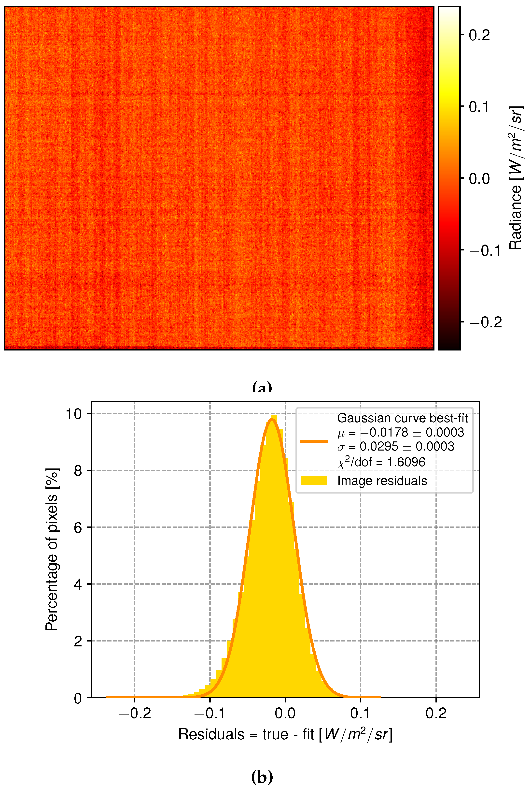
Figure 12.
(a) Colormap displaying the residuals between a calculated scene radiance and a calibrated blackbody image in . The fixed pattern noise (FPN) appears as vertical stripes. (b) Histogram distribution of pixel radiance residuals with a Gaussian fit curve. The fitted sigma value 0.029 is close to the NERD = 0.0260 for this scene radiance.
3.4. Application to Sky Radiance Images
To evaluate the efficiency of the calibration model, we compare simulations with radiances of sky images acquired across multiple nights. A series of simulations using libRadTran radiative transfer code [42] were run for three standard atmosphere profiles at a base altitude of 650 m above sea-level: midlatitude summer, winter and US76 [43]. Air pressure and ground temperature were measured on-site with a dedicated weather station. Ozone concentration and satellite-based PWV measurements were retrieved from the ERA5 dataset [44] using the cdsapi7 package. All of these parameters were given as input for each simulation, corresponding to one image acquired at a specific time and zenith angle during the night. The framework computes the atmospheric spectral radiance which was then integrated over the throughput curve shown in Figure 4. Sequences were cautiously selected to be free of apparent clouds, and across a sufficient airmass range. We used the DISORT (DIScrete Ordinate Radiative Transfer) method to solve the radiative transfer equation in plane-parallel approximation [42], as zenith angles stayed below 45°. As the full image FOV is large, we focus here on a small fraction that matches the line of sight of the StarDICE optical photometry telescope. The observed radiance is calculated as the mean of a crop area of 32 × 32 pixels near the center of the image, each pixel being close to 1 arcmin across. Figure 13 shows downward spectral radiances computed between 6.5 and 15 µm. Figure 13 depicts the corresponding radiances integrated over the instrument throughput. They can be used to quantify the impact of changes in PWV on downward radiances for a fixed atmosphere. The integrated scene radiance is intended to simulate our thermal sensor’s calibrated reading. A higher PWV amount leads to higher sky radiances, which can be interpreted as a lowering in altitude of the effective emission level due to increased water vapor opacity, with lower altitudes generally corresponding to higher temperatures [45].
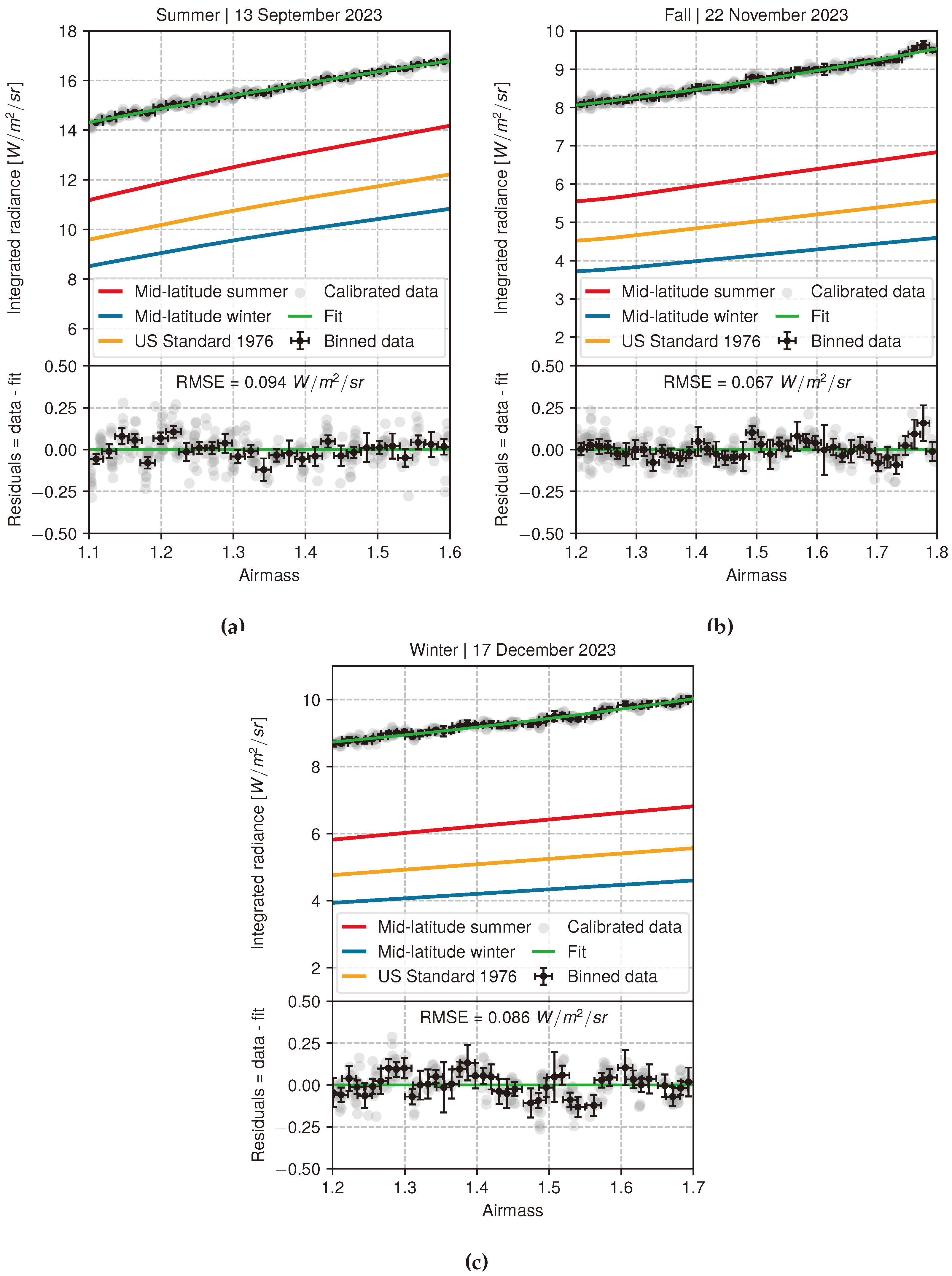
Figure 14 presents the comparison of calibrated radiance data and simulations for three nights of 2023 northern hemisphere summer (September 13), fall (November 22), and winter (December 17). Default atmosphere profiles of mid-latitude summer, winter, and US 76 standard models were used as input to libRadTran simulations with the PWV integral column normalized to the value measured by satellite observations from ERA5 dataset. The radiance increase with airmass is well reproduced by our calibrated data. The residuals between the calibrated data and a fitted second-order polynomial curve (green) are shown in the lower panels. The small dispersion, with RMSE values below 0.1 , indicates excellent smoothness of the data for a clear sky and matches the results of the calibration experiment. The simulated values are systematically below the calibrated observations envelope for all models in Fig. Figure 14 (summer), Figure 14 (fall) and Figure 14 (winter), with average PWV values of 24.98 mm, 6.29 mm and 7.27 mm respectively. The mid-latitude summer model is closest to experimental data with a global offset of 2.5 from the mid-latitude summer model across the three datasets and could be explained by the presence of a warm foreground. Indeed, the instrument is placed on an equatorial mount inside a dome. None of the standard atmospheric profiles adjusts the real conditions. Nevertheless, our findings align closely with those of Hack et al. [23], who observed biases towards smaller radiance values in simulations using standard atmosphere profiles. They demonstrated the significance of the vertical distribution of water vapor content with radiosonde profiles taken above their specific site. Measurements of PWV from satellite observations are not precise enough due to the temporal (i.e., 1 hour) and spatial horizontal (0.25 × 0.25°) resolutions. Additional instruments such as a GNSS receiver may be required to properly measure the local value of PWV with 1 mm accuracy [46].
4. Discussion
4.1. Bias in Scene Radiance Estimation
The use of a forward model to estimate scene radiance through the use of Equation 6, while effective within the defined constraints, incorporates simplifications that may not fully capture the intricacies of heat transfer and environmental exchanges. Any deviation from the model’s assumptions can introduce systematic bias. The potential for over- or underestimation under specific environmental conditions unaccounted for in the model raises concerns about the validity of the calibration when using the camera in real-world settings outside the calibration environmental conditions. Low-level sky radiance measurements may suffer from biases. Furthermore, the radiance range the camera encounters during on-sky measurements differs from that available during calibration. As a result, calibration may need to be extrapolated beyond this range (12-30 ) for on-sky measurements and may lead to errors when assessing the true scene radiance. In Section 2.7, we discussed the impact of ambient radiation variation in the laboratory setup. It required to introduce the additional term fitted with parameter. For on-sky observations, in an open environment, this term will not impact our measurements and is thus not applied for calibrating the associated images. However, in the on-sky observations presented in Fig. Figure 14, similar complications may arise due to the emission of the dome hosting the experiment. In an attempt to efficiently deal with this issue the experiment has recently been moved to an entirely open building.
4.2. Remaining Fixed Pattern Noise in Calibrated Images
In Figure 12 some remaining structures appearing as vertical stripes persist. The dispersion of these residuals ( ) is very close to the Noise Equivalent Radiance Difference (NERD) value (0.0260 ) provided by the manufacturer. The UIRTC used in this work has a read-out electronics similar to an optical CMOS-based camera. A shift from chip-level to column-level analog-to-digital converter (ADC) has been adopted, allowing for lower-speed and lower-power operation. However, this approach introduces column fixed pattern noise (FPN), compromising image quality. This effect originates from the mismatch between electronic gain and bias of ADC channels [47]. These parameters temporally fluctuate. Therefore, the residual structure is always spatially evolving and FPN remains visible even after subtracting two consecutive images. Existing complementary image post-processing methods involving deconvolution [48] or neural networks [49] can significantly reduce this residual artifact, but are beyond the scope of the presented work.
4.3. Non-Linearity Correction in Pixel Response
Any detector’s response is not linear for its entire operation regime and deviates at the edges [34]. As a result, the linear approximation is no longer valid as the response saturates at the upper end and stagnates at a non-zero bias level for the lower end. This non-linearity is partially caused by the read-out electronics [34,50]. Multiple expressions to model the non-linearity function have been proposed. Zhou et al. [51] proposed a fixed S-shape curve formulation with the natural logarithm: , with BD being the bit-depth of the sensor ( for our instrument). Lane and Whitenton [34] took the linearity fit equation from Saunders and White [52] with 4 parameters to adjust (considering the gain k): with . Other models employing polynomials are also worth studying. If one were interested in higher radiance levels, up to the saturation limit of the sensor, a logistic function model may be preferred. Nevertheless, it is important to note that accurately mapping non-linearity requires measurements across the sensor’s entire sensitivity range, which was not possible with our experimental setup.
4.4. Correlation between Scene Radiance and Camera Temperature
The origin of the degeneracy between ambient and FPA temperatures lies in the environmental conditions shared by the sensor and the scene. The ambient temperature influences the scene radiance captured by the camera through reflections on the blackbody source, and it affects the temperature of the camera’s FPA. This co-dependence challenges radiometric calibration, as changes in ambient temperature lead to simultaneous variations in FPA temperature, creating a degenerate relationship between these two variables. Consequently, distinguishing the specific impact of each temperature becomes intricate, with covariances and correlations that complicate the accurate determination of model parameters during the calibration process.
An effective strategy to mitigate this challenge involves placing the camera within a climatic chamber, equipped with an aperture for external exposure. This setup can incorporate moving blackbody sources, akin to the calibration bench used by Lin et al. [53]. Such a configuration offers the potential to disentangle the influence of ambient and FPA temperatures, facilitating more accurate and robust calibration procedures. However, replicating the calibration setup with a climatic chamber and moving blackbody sources proved unfeasible in our study due to limitations in infrastructure, and budget and time constraints.
5. Conclusions
In this study, we have presented a comprehensive calibration procedure suitable for a UIRTC and aimed at improving its performance to measure the sky downwelling radiance and detect cirrus clouds. A dedicated calibration bench using a climatic chamber and a thermoregulated blackbody source was set up to calibrate the FLIR Tau2 IR thermal camera. A specific analytical calibration model relying on radiance was used. The scene radiance was estimated with a tailored forward model approach. It demonstrated excellent accuracy regarding the average RMSE and the spatial noise. We created matrices of calibration coefficients that will be applied to raw images later on for on-site measurements. The calibration delivers a radiometric precision better than 0.1 for each pixel of the instrument FPA. After calibration, spatial noise is found to be roughly equal to the manufacturer’s NERD at ∼ 0.03 . Applying the following additional adjustments may further improve the results and facilitate the analysis: (i) increase the time duration of climatic chamber temperature set points to let the camera temperature stabilize even more; (ii) use a larger climatic chamber in combination with a larger blackbody emitting surface to increase its distance to the camera and reduce convective and radiative heat transfers between instruments; (iii) consider additional blackbody temperature set-points at lower temperatures; (iv) extend the climatic chamber temperature range; (v) repeat the measurements multiple times and/or regularly to evaluate repeatability and variations in time. Further work could focus on the correction of the remaining FPN by incorporating additional reduction process. Additional nights of data collection will occur at Observatoire de Haute-Provence for the StarDICE experiment. In parallel to IR radiometric measurements, high-precision optical photometry, and spectrophotometry of reference stars is being performed. Future work will focus on establishing a joint analysis between LWIR radiometric images and visible to near-IR photometric data. We hypothesize that by combining on-site and off-site high-accuracy atmosphere sensing (LIDAR [54,55], weather stations, local AERONET data [56,57,58], satellite data [59] and GNSS PWV measurements [60]), it will be possible to: (i) improve the modelling of the sky background radiance of LWIR images using libRadTran [42] and isolate any cloud structure after PWV emission subtraction [61]; (ii) quantify the optical photometric flux loss due to atmospheric gray extinction variations.
Author Contributions
Conceptualization, K.S. and B.P.; methodology, K.S., B.P and J.C-T.; software, K.S., B.P., and M.B.; formal analysis, K.S. and B.P.; resources, K.S., S.D-G., M.M; data collection for calibration experiment; K.S., S.D-G., M.M; data collection for on-sky measurements, K.S., M.B. and S.B.; data curation, investigation, K.S., B.P., S.D-G., M.M, J.N.; writing—original draft preparation, K.S., B.P.; writing—review and editing, B.P., J.C-T., S.D-G., M.M, J.N., M.B., S.B., F.F., L.L.G., T.S. All authors have read and agreed to the published version of the manuscript.
Funding
This work received support from the Programme National Cosmology et Galaxies (PNCG) of CNRS/INSU with INP and IN2P3, co-funded by CEA and CNES and from the DIM ACAV program of the Île-de-France region.
Data Availability Statement
The data presented in this study are available on request from the corresponding author.
Acknowledgments
We thank Ana Torrento, Marc Escalier, Adbelali Slimani-Cherif for their time and availability to perform the calibration measurements. This work was completed in part with resources provided by Laboratoire de Physique des 2 infinis Irène Joliot-Curie – IJCLab UMR9012 – CNRS / Université Paris-Saclay / Université Paris Cité. We also thank Stéphane Nou from Laboratoire Univers et Particules de Montpellier CNRS/IN2P3 for facilitating our high-performance computing endeavors required to process the large amount of calibration data. Some of the results in this paper have been derived using astropy [62], iminuit [40], numba [63], numpy [64], and scipy [65] packages. Figures in this article have been created using matplotlib [66].
Conflicts of Interest
The authors declare no conflict of interest. The funders had no role in the design of the study; in the collection, analyses, or interpretation of data; in the writing of the manuscript; or in the decision to publish the results.
Abbreviations
The following abbreviations are used in this manuscript:
| ADC | Analog-to-Digital Converter |
| ADU | Analog-to-Digital Units |
| BD | Bit-depth |
| CMOS | Complementary Metal-Oxide-Semiconductor |
| DSNU | Dark Signal Non-Uniformity |
| FFC | Flat-Field Correction |
| FOV | Field-of-View |
| FPA | Focal Plane Array |
| FPGA | Field-Programmable Gate Array |
| FPN | Fixed Pattern Noise |
| IR | Infrared |
| LWIR | Long-Wave Infrared |
| NETD | Noise Equivalent Temperature Difference |
| NERD | Noise Equivalent Radiance Difference |
| NIST | National Institute of Standards and Technology |
| NUC | Non-uniformity Correction |
| PRNU | Pixel Response Non-Uniformity |
| PWV | Precipitable Water Vapor |
| RMSE | Root-Mean Square Error |
| SNR | Signal-to-Noise Ratio |
| UIRTC | Uncooled Infrared Thermal Camera |
References
- Magnier, E.A.; Schlafly, E.F.; Finkbeiner, D.P.; Tonry, J.L.; Goldman, B.; Röser, S.; Schilbach, E.; Casertano, S.; Chambers, K.C.; Flewelling, H.A.; Huber, M.E.; Price, P.A.; Sweeney, W.E.; Waters, C.Z.; Denneau, L.; Draper, P.W.; Hodapp, K.W.; Jedicke, R.; Kaiser, N.; Kudritzki, R.P.; Metcalfe, N.; Stubbs, C.W.; Wainscoat, R.J. Pan-STARRS Photometric and Astrometric Calibration. [arXiv:astro-ph.IM/1612.05242]. 2020, 251, 6. [Google Scholar] [CrossRef]
- Rykoff, E.S.; Tucker, D.L.; Burke, D.L.; Allam, S.S.; Bechtol, K.; Bernstein, G.M.; Brout, D.; Gruendl, R.A.; Lasker, J.; Smith, J.A.; Wester, W.C.; Yanny, B.; Abbott, T.M.C.; Aguena, M.; Alves, O.; Andrade-Oliveira, F.; Annis, J.; Bacon, D.; Bertin, E.; Brooks, D.; Carnero Rosell, A.; Carretero, J.; Castander, F.J.; Choi, A.; da Costa, L.N.; Pereira, M.E.S.; Davis, T.M.; De Vicente, J.; Diehl, H.T.; Doel, P.; Drlica-Wagner, A.; Everett, S.; Ferrero, I.; Frieman, J.; García-Bellido, J.; Giannini, G.; Gruen, D.; Gutierrez, G.; Hinton, S.R.; Hollowood, D.L.; James, D.J.; Kuehn, K.; Lahav, O.; Marshall, J.L.; Mena-Fernández, J.; Menanteau, F.; Myles, J.; Nord, B.D.; Ogando, R.L.C.; Palmese, A.; Pieres, A.; Plazas Malagón, A.A.; Raveri, M.; Rodgríguez-Monroy, M.; Sanchez, E.; Santiago, B.; Schubnell, M.; Sevilla-Noarbe, I.; Smith, M.; Soares-Santos, M.; Suchyta, E.; Swanson, M.E.C.; Varga, T.N.; Vincenzi, M.; Walker, A.R.; Weaverdyck, N.; Wiseman, P. The Dark Energy Survey Six-Year Calibration Star Catalog. arXiv e-prints 2023. p. arXiv:2305.01695, [arXiv:astro-ph.IM/2305.01695]. [Google Scholar] [CrossRef]
- Ivezić. ; others. LSST: From Science Drivers to Reference Design and Anticipated Data Products. 2019, arXiv:astro-ph/0805.2366]873, 111. [CrossRef]
- Stubbs, C.W.; High, F.W.; George, M.R.; DeRose, K.L.; Blondin, S.; Tonry, J.L.; Chambers, K.C.; Granett, B.R.; Burke, D.L.; Smith, R.C. Toward More Precise Survey Photometry for PanSTARRS and LSST: Measuring Directly the Optical Transmission Spectrum of the Atmosphere. Publications of the Astronomical Society of the Pacific 2007, 119, 1163–1178. [Google Scholar] [CrossRef]
- Collaboration, D.E.S. The LSST Dark Energy Science Collaboration (DESC) Science Requirements Document. 2018, arXiv:1809.01669. [Google Scholar]
- Betoule, M.; Antier, S.; Bertin, E.; Blanc, P.É.; Bongard, S.; Cohen Tanugi, J.; Dagoret-Campagne, S.; Feinstein, F.; Hardin, D.; Juramy, C.; Le Guillou, L.; Le Van Suu, A.; Moniez, M.; Neveu, J.; Nuss, É.; Plez, B.; Regnault, N.; Sepulveda, E.; Sommer, K.; Souverin, T.; Wang, X.F. StarDICE. I. Sensor calibration bench and absolute photometric calibration of a Sony IMX411 sensor. [arXiv:astro-ph.IM/2211.04913]. 2023, 670, A119. [Google Scholar] [CrossRef]
- Bohlin, R.C.; Hubeny, I.; Rauch, T. New Grids of Pure-hydrogen White Dwarf NLTE Model Atmospheres and the HST/STIS Flux Calibration. The Astronomical Journal 2020, 160, 21. [Google Scholar] [CrossRef]
- Larason, T.; Houston, J. Spectroradiometric Detector Measurements: Ultraviolet, Visible, and Near Infrared Detectors for Spectral Power, 2008.
- LSST Science Collaboration. LSST Science Book, Version 2.0. arXiv e-prints p. arXiv:0912.0201, [arXiv:astro-ph.IM/0912.0201]. 2009, arXiv:0912.0201.
- Hazenberg, F. Calibration photométrique des supernovae de type Ia pour la caractérisation de l’énergie noire avec l’expérience StarDICE. Theses, Sorbonne Université, 2019.
- Burke, D.L.; Saha, A.; Claver, J.; Axelrod, T.; Claver, C.; DePoy, D.; Ivezić, Ž.; Jones, L.; Smith, R.C.; Stubbs, C.W. ALL-WEATHER CALIBRATION OF WIDE-FIELD OPTICAL AND NIR SURVEYS. The Astronomical Journal 2013, 147, 19. [Google Scholar] [CrossRef]
- Burke, D.L.; Rykoff, E.S.; Allam, S.; Annis, J.; Bechtol, K.; Bernstein, G.M.; Drlica-Wagner, A.; Finley, D.A.; Gruendl, R.A.; James, D.J.; Kent, S.; Kessler, R.; Kuhlmann, S.; Lasker, J.; Li, T.S.; Scolnic, D.; Smith, J.; Tucker, D.L.; Wester, W.; Yanny, B.; Abbott, T.M.C.; Abdalla, F.B.; Benoit-Levy, A.; Bertin, E.; Rosell, A.C.; Kind, M.C.; Carretero, J.; Cunha, C.E.; D’Andrea, C.B.; da Costa, L.N.; Desai, S.; Diehl, H.T.; Doel, P.; Estrada, J.; Garcia-Bellido, J.; Gruen, D.; Gutierrez, G.; Honscheid, K.; Kuehn, K.; Kuropatkin, N.; Maia, M.A.G.; March, M.; Marshall, J.L.; Melchior, P.; Menanteau, F.; Miquel, R.; Plazas, A.A.; Sako, M.; Sanchez, E.; Scarpine, V.; Schindler, R.; Sevilla-Noarbe, I.; Smith, M.; Smith, R.C.; Soares-Santos, M.; Sobreira, F.; Suchyta, E.; Tarle, G.; and, A.R.W. Forward Global Photometric Calibration of the Dark Energy Survey. The Astronomical Journal 2017, 155, 41. [Google Scholar] [CrossRef]
- Szejwach, G. Determination of Semi-Transparent Cirrus Cloud Temperature from Infrared Radiances: Application to METEOSAT. Journal of Applied Meteorology and Climatology 1982, 21, 384–393. [Google Scholar] [CrossRef]
- Shaw, J.A.; Nugent, P.W. Physics principles in radiometric infrared imaging of clouds in the atmosphere. European Journal of Physics 2013, 34, S111–S121. [Google Scholar] [CrossRef]
- Liandrat, O.; Cros, S.; Braun, A.; Saint-Antonin, L.; Decroix, J.; Schmutz, N. Cloud cover forecast from a ground-based all sky infrared thermal camera. Remote Sensing of Clouds and the Atmosphere XXII. SPIE, 2017, Vol. 10424, pp. 19–31.
- Lopez, T.; Antoine, R.; Baratoux, D.; Rabinowicz, M. Contribution of thermal infrared images on the understanding of the subsurface/atmosphere exchanges on Earth. EGU General Assembly Conference Abstracts, 2017, p. 11811.
- Klebe, D.I.; Blatherwick, R.D.; Morris, V.R. Ground-based all-sky mid-infrared and visible imagery for purposes of characterizing cloud properties. Atmospheric Measurement Techniques 2014, 7, 637–645. [Google Scholar] [CrossRef]
- Nikolenko, I.; Maslov, I. Infrared (thermal) camera for monitoring the state of the atmosphere above the sea horizon of the Simeiz Observatory INASAN. INASAN Science Reports 2021, 6, 85–87. [Google Scholar]
- Shaw, J.A.; others. Radiometric cloud imaging with an uncooled microbolometer thermal infrared camera. Optics Express 2005, 13, 5807. [Google Scholar] [CrossRef]
- Brocard, E.; others. Detection of Cirrus Clouds Using Infrared Radiometry. IEEE Transactions on Geoscience and Remote Sensing 2011, 49, 595–602. [Google Scholar] [CrossRef]
- Sebag, J.; Andrew, J.; Klebe, D.; Blatherwick, R. LSST all-sky IR camera cloud monitoring test results. Proceedings of SPIE - The International Society for Optical Engineering 2010, 7733. [Google Scholar] [CrossRef]
- Lewis, P.M.; Rogers, H.; Schindler, R.H. A radiometric all-sky infrared camera (RASICAM) for DES/CTIO. Ground-based and Airborne Instrumentation for Astronomy III. SPIE, 2010, Vol. 7735, pp. 1307–1318.
- Hack, E.D.; Pauliquevis, T.; Barbosa, H.M.J.; Yamasoe, M.A.; Klebe, D.; Correia, A.L. Precipitable water vapor retrievals using a ground-based infrared sky camera in subtropical South America. Atmospheric Measurement Techniques 2023, 16, 1263–1278. [Google Scholar] [CrossRef]
- Poissenot-Arrigoni, C.; Marcon, B.; Rossi, F.; Fromentin, G. Fast and easy radiometric calibration method integration time insensitive for infrared thermography. Infrared Physics & Technology 2023, 133, 104741. [Google Scholar] [CrossRef]
- Nugent, P.W.; others. Correcting for focal-plane-array temperature dependence in microbolometer infrared cameras lacking thermal stabilization. Optical Engineering 2013, 52, 061304. [Google Scholar] [CrossRef]
- Ribeiro-Gomes, K.; Hernández-López, D.; Ortega, J.F.; Ballesteros, R.; Poblete, T.; Moreno, M.A. Uncooled Thermal Camera Calibration and Optimization of the Photogrammetry Process for UAV Applications in Agriculture. Sensors 2017, 17. [Google Scholar] [CrossRef] [PubMed]
- González-Chávez, O.; Cárdenas-Garcia, D.; Karaman, S.; Lizárraga, M.; Salas, J. Radiometric Calibration of Digital Counts of Infrared Thermal Cameras. IEEE Transactions on Instrumentation and Measurement 2019, 68, 4387–4399. [Google Scholar] [CrossRef]
- Benirschke, D.; Howard, S. Characterization of a low-cost, commercially available, vanadium oxide microbolometer array for spectroscopic imaging. Optical Engineering 2017, 56, 040502. [Google Scholar] [CrossRef]
- Avdelidis, N.; Moropoulou, A. Emissivity considerations in building thermography. Energy and Buildings 2003, 35, 663–667. [Google Scholar] [CrossRef]
- Vu, L. Nguyen.; Flir Systems. Flat field correction for infrared cameras, U.S. Patent US8373757B1 2009.
- Joseph, L. Kostrzewa.; Vu L. Nguyen.; Theodore R. Hoelter.; Flir Systems. Flat field correction for infrared cameras, U.S. Patent US20130147966A1 2013.
- Mudau, A.E.; Willers, C.J.; Griffith, D.; le Roux, F.P. Non-uniformity correction and bad pixel replacement on LWIR and MWIR images. 2011 Saudi International Electronics, Communications and Photonics Conference (SIECPC). IEEE, 2011, pp. 1–5.
- Budzier, H.; Gerlach, G. Calibration of uncooled thermal infrared cameras. Journal of Sensors and Sensor Systems 2015, 4, 187–197. [Google Scholar] [CrossRef]
- Lane, B.; Whitenton, E. Calibration and measurement procedures for a high magnification thermal camera. Report no. NISTIR8098 (National Institute of Standards and Technology, Gaithersburg, MD, 2015) 2015.
- Tempelhahn, A.; Budzier, H.; Krause, V.; Gerlach, G. Shutter-less calibration of uncooled infrared cameras. Journal of Sensors and Sensor Systems 2016, 5, 9–16. [Google Scholar] [CrossRef]
- Tempelhahn, A.; Budzier, H.; Krause, V.; Gerlach, G. P3-Modeling Signal-Determining Radiation Components of Microbolometer-Based Infrared Measurement Systems. Proceedings IRS2 2013, 2013, 100–104. [Google Scholar]
- Bhan, R.; Saxena, R.; Jalwania, C.; Lomash, S. Uncooled Infrared Microbolometer Arrays and their Characterisation Techniques. Defence Science Journal 2009, 59, 580. [Google Scholar] [CrossRef]
- Guadagnoli, E.; Giunti, C.; Mariani, P.; Olivieri, M.; Porta, A.; Sozzi, B.; Zatti, S. Thermal imager non-uniformity sources modeling. Infrared Imaging Systems: Design, Analysis, Modeling, and Testing XXII. SPIE, 2011, Vol. 8014, pp. 88–99.
- Efron, B. Better Bootstrap Confidence Intervals. Journal of the American Statistical Association 1987, 82, 171–185. [Google Scholar] [CrossRef]
- Dembinski, H.; et al., P.O. scikit-hep/iminuit. 2020. [CrossRef]
- Howard, J.W.; Abel, I.R. Narcissus: reflections on retroreflections in thermal imaging systems. Applied Optics 1982, 21, 3393–3397. [Google Scholar] [CrossRef] [PubMed]
- Emde, C.; Buras-Schnell, R.; Kylling, A.; Mayer, B.; Gasteiger, J.; Hamann, U.; Kylling, J.; Richter, B.; Pause, C.; Dowling, T.; Bugliaro, L. The libRadtran software package for radiative transfer calculations (version 2.0.1). Geoscientific Model Development 2016, 9, 1647–1672. [Google Scholar] [CrossRef]
- Anderson, G.P.; Clough, S.A.; Kneizys, F.X.; Chetwynd, J.H.; Shettle, E.P. AFGL (Air Force Geophysical Laboratory) atmospheric constituent profiles (0. 120km). Environmental research papers.
- Hersbach, H.; Bell, B.; Berrisford, P.; Biavati, G.; Horányi, A.; Muñoz Sabater, J.; Nicolas, J.; Peubey, C.; Radu, R.; Rozum, I.; Schepers, D.; Simmons, A.; Soci, C.; Dee, D.; Thépaut, J.N. ERA5 hourly data on single levels from 1940 to present. Copernicus Climate Change Service (C3S) Climate Data Store (CDS), 2023. Accessed on DD-MMM-YYYY. [CrossRef]
- Kelsey, V.; Riley, S.; Minschwaner, K. Atmospheric precipitable water vapor and its correlation with clear-sky infrared temperature observations. Atmospheric Measurement Techniques 2022, 15, 1563–1576. [Google Scholar] [CrossRef]
- Sugiyama, J.; Nishino, H.; Kusaka, A. Precipitable water vapour measurement using GNSS data in the Atacama Desert for millimetre and submillimetre astronomical observations. Monthly Notices of the Royal Astronomical Society 2024, 528, 4582–4590. [Google Scholar] [CrossRef]
- Snoeij, M.F.; Theuwissen, A.J.P.; Makinwa, K.A.A.; Huijsing, J.H. A CMOS Imager With Column-Level ADC Using Dynamic Column Fixed-Pattern Noise Reduction. IEEE Journal of Solid-State Circuits 2006, 41, 3007–3015. [Google Scholar] [CrossRef]
- Lee, H.; Kang, M.G. Infrared Image Deconvolution Considering Fixed Pattern Noise. Sensors 2023, 23. [Google Scholar] [CrossRef] [PubMed]
- Guan, J.; Lai, R.; Xiong, A.; Liu, Z.; Gu, L. Fixed pattern noise reduction for infrared images based on cascade residual attention CNN. Neurocomputing 2020, 377, 301–313. [Google Scholar] [CrossRef]
- Schulz, M.; Caldwell, L. Nonuniformity correction and correctability of infrared focal plane arrays. Infrared physics & technology 1995, 36, 763–777. [Google Scholar] [CrossRef]
- Zhou, H.; Liu, S.; Lai, R.; Wang, D.; Cheng, Y. Solution for the nonuniformity correction of infrared focal plane arrays. Appl. Opt. 2005, 44, 2928–2932. [Google Scholar] [CrossRef]
- Saunders, P.; White, D. Propagation of Uncertainty Due to Non-linearity in Radiation Thermometers. International Journal of Thermophysics 2007, 28, 2098–2110. [Google Scholar] [CrossRef]
- Lin, D.; Cui, X.; Wang, Y.; Yang, B.; Tian, P. Pixel-wise radiometric calibration approach for infrared focal plane arrays using multivariate polynomial correction. Infrared Physics & Technology 2022, 123, 104110. [Google Scholar] [CrossRef]
- Bock, O.; Bosser, P.; Bourcy, T.; David, L.; Goutail, F.; Hoareau, C.; Keckhut, P.; Legain, D.; Pazmino, A.; Pelon, J.; Pipis, K.; Poujol, G.; Sarkissian, A.; Thom, C.; Tournois, G.; Tzanos, D. Accuracy assessment of water vapour measurements from in situ and remote sensing techniques during the DEMEVAP 2011 campaign at OHP. Atmospheric Measurement Techniques 2013, 6, 2777–2802. [Google Scholar] [CrossRef]
- Khaykin, S.M.; Godin-Beekmann, S.; Keckhut, P.; Hauchecorne, A.; Jumelet, J.; Vernier, J.P.; Bourassa, A.; Degenstein, D.A.; Rieger, L.A.; Bingen, C.; Vanhellemont, F.; Robert, C.; DeLand, M.; Bhartia, P.K. Variability and evolution of the midlatitude stratospheric aerosol budget from 22 years of ground-based lidar and satellite observations. Atmospheric Chemistry and Physics 2017, 17, 1829–1845. [Google Scholar] [CrossRef]
- Holben, B.; Eck, T.; Slutsker, I.; Tanré, D.; Buis, J.; Setzer, A.; Vermote, E.; Reagan, J.; Kaufman, Y.; Nakajima, T.; Lavenu, F.; Jankowiak, I.; Smirnov, A. AERONET—A Federated Instrument Network and Data Archive for Aerosol Characterization. Remote Sensing of Environment 1998, 66, 1–16. [Google Scholar] [CrossRef]
- Rogozovsky, I.; Ansmann, A.; Althausen, D.; Heese, B.; Engelmann, R.; Hofer, J.; Baars, H.; Schechner, Y.; Lyapustin, A.; Chudnovsky, A. Impact of aerosol layering, complex aerosol mixing, and cloud coverage on high-resolution MAIAC aerosol optical depth measurements: Fusion of lidar, AERONET, satellite, and ground-based measurements. Atmospheric Environment 2021, 247, 118163. [Google Scholar] [CrossRef]
- Kelsey, V.; Riley, S.; Minschwaner, K. Atmospheric precipitable water vapor and its correlation with clear-sky infrared temperature observations. Atmospheric Measurement Techniques 2022, 15, 1563–1576. [Google Scholar] [CrossRef]
- Meier Valdés, E. A. .; Morris, B. M..; Demory, B.-O.. Monitoring precipitable water vapour in near real-time to correct near-infrared observations using satellite remote sensing. A&A 2021, 649, A132. [Google Scholar] [CrossRef]
- Sugiyama, J.; Nishino, H.; Kusaka, A. Precipitable Water Vapor Measurement using GNSS Data in the Atacama Desert for Millimeter and Submillimeter Astronomical Observations, 2023, [arXiv:astro-ph.IM/2308.12632].
- Thurairajah, B.; Shaw, J. Cloud statistics measured with the infrared cloud imager (ICI). IEEE Transactions on Geoscience and Remote Sensing 2005, 43, 2000–2007. [Google Scholar] [CrossRef]
- Astropy Collaboration, T. Astropy: A community Python package for astronomy. AJ 2018, 156, 123. [Google Scholar] [CrossRef]
- Lam, S.K.; Pitrou, A.; Seibert, S. Numba: A llvm-based python jit compiler. Proceedings of the Second Workshop on the LLVM Compiler Infrastructure in HPC, 2015, pp. 1–6.
- Harris, C.R.; Millman, K.J.; van der Walt, S.J.; Gommers, R.; Virtanen, P.; Cournapeau, D.; Wieser, E.; Taylor, J.; Berg, S.; Smith, N.J.; Kern, R.; Picus, M.; Hoyer, S.; van Kerkwijk, M.H.; Brett, M.; Haldane, A.; del Rio, J.F.; Wiebe, M.; Peterson, P.; Gerard-Marchant, P.; Sheppard, K.; Reddy, T.; Weckesser, W.; Abbasi, H.; Gohlke, C.; Oliphant, T.E. Array programming with NumPy. Nature 2020, 585, 357–362. [Google Scholar] [CrossRef]
- Virtanen, P.; Gommers, R.; Oliphant, T.E.; Haberland, M.; Reddy, T.; Cournapeau, D.; Burovski, E.; Peterson, P.; Weckesser, W.; Bright, J.; van der Walt, S.J.; Brett, M.; Wilson, J.; Millman, K.J.; Mayorov, N.; Nelson, A.R.J.; Jones, E.; Kern, R.; Larson, E.; Carey, C.J.; Polat, İ.; Feng, Y.; Moore, E.W.; VanderPlas, J.; Laxalde, D.; Perktold, J.; Cimrman, R.; Henriksen, I.; Quintero, E.A.; Harris, C.R.; Archibald, A.M.; Ribeiro, A.H.; Pedregosa, F.; van Mulbregt, P. SciPy 1.0 Contributors. SciPy 1.0: Fundamental Algorithms for Scientific Computing in Python. Nature Methods 2020, 17, 261–272. [Google Scholar] [CrossRef] [PubMed]
- Hunter, J.D. CSE2007, 9, 90. [CrossRef]
| 1 | The f#-number is defined as the ratio of the focal length to the diameter of the aperture. |
| 2 | |
| 3 | |
| 4 | |
| 5 | Code for the FLIR Tau2 camera with TeAx ThermalGrabber https://github.com/Kelian98/tau2_thermalcapture
|
| 6 | Code for the IR2101 blackbody https://github.com/Kelian98/ir2101_blackbody
|
| 7 |
Figure 1.
Flowchart of the calibration process represented in two distinct blocks. The left block represents the laboratory calibration experiment on a reference blackbody source in controlled environmental conditions. The right block represents the application of the calibration model to raw data during operations, producing true radiance radiometric images.
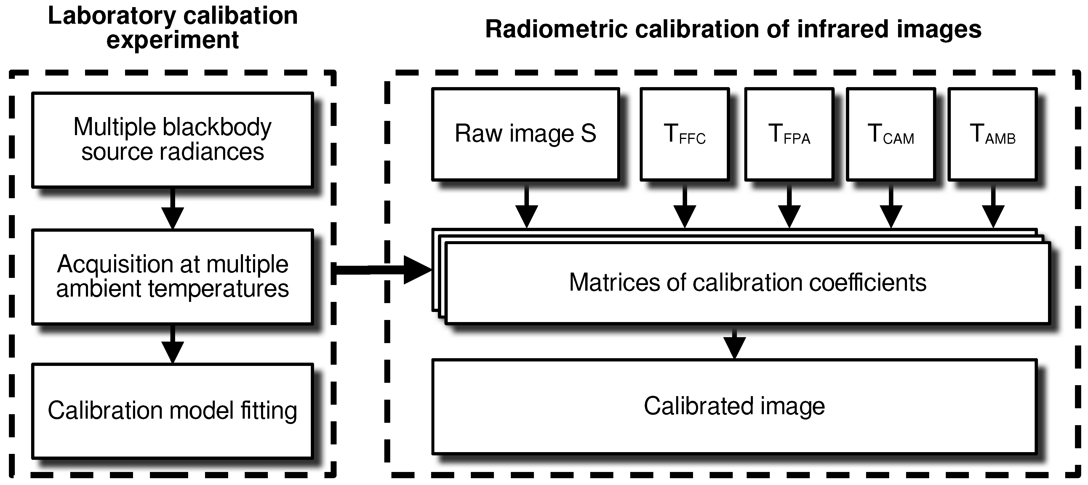
Figure 2.
(a) Picture of the entire calibration setup. The climatic chamber stands on the right side of the picture. The blackbody source controller stands on the center of the image. On top sits the Raspberry Pi 4 accessed through SSH with the desktop PC on the left. Cables for the IR camera, temperature sensors, and blackbody emitting surface area pass through the climatic chamber within the intended cable sleeve. (b) Annotated photo of the interior of the climatic chamber. The camera is attached to a telescope dovetail bar facing the blackbody target with the flat-field support in operation position. The temperature sensor is attached onto a non-moving plate emulating the FFC plate to prevent mechanical issues due to moving cables.
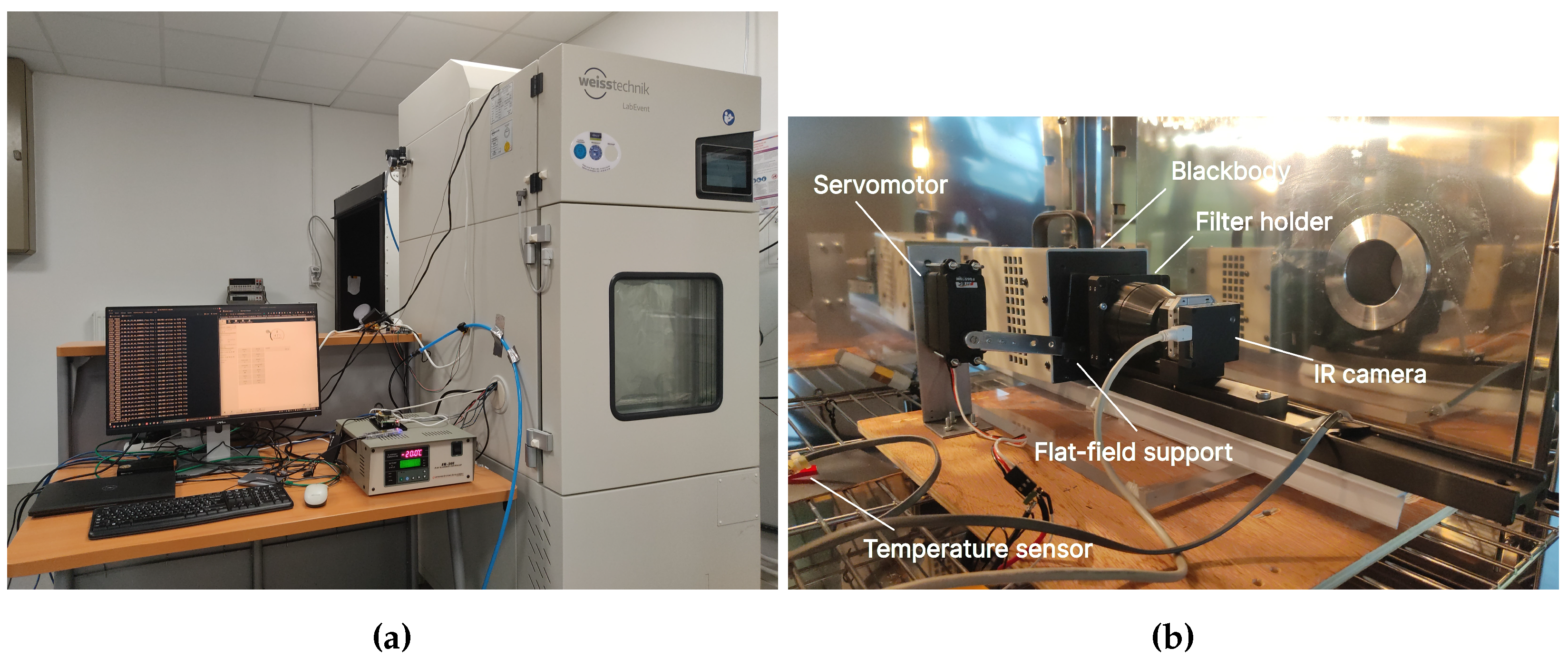
Figure 3.
Sketch of the calibration setup bench. The blackbody source is thermoregulated by its controller sitting outside the climatic chamber. The red circles represent additional temperature sensors. The orange circles represent temperature sensors already installed inside the camera and whose readings are obtained through the software. The connecting lines depict communication for data transfer and control/command. The Raspberry Pi 4 microcomputer controls the entire setup and stores data on an SSD.
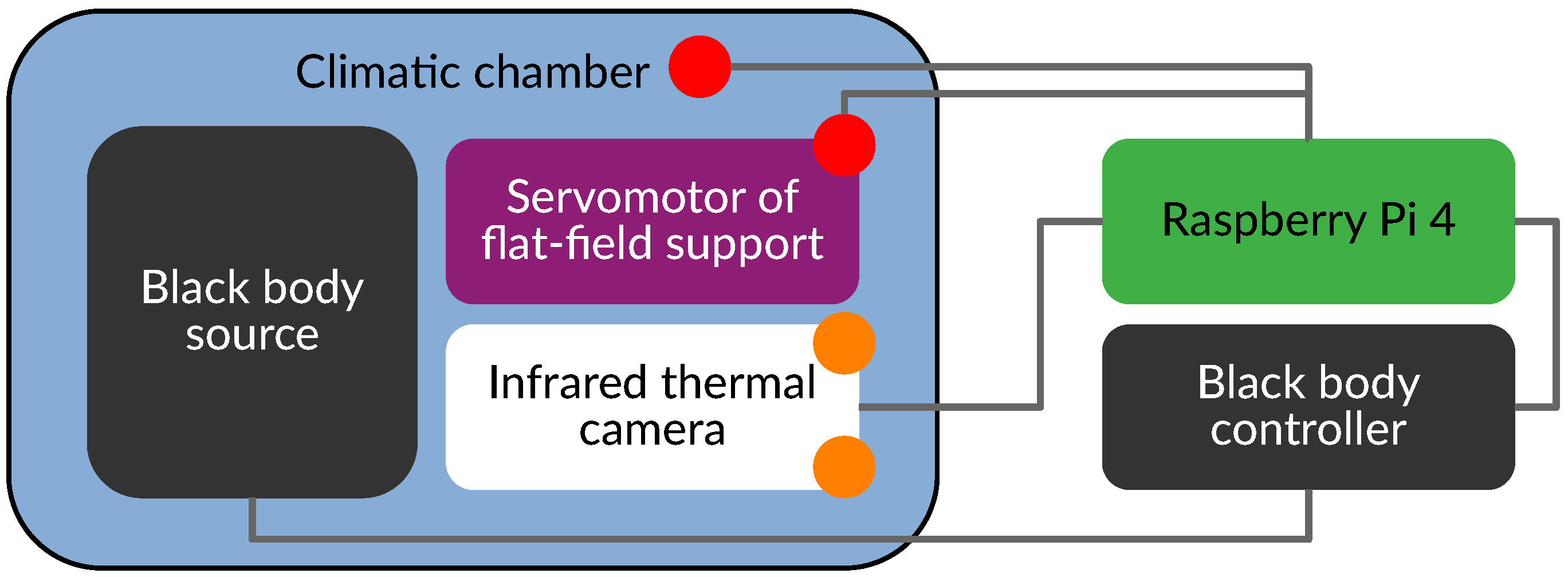
Figure 4.
Spectral responses of the FLIR Tau 2 camera core and Umicore F#1.25 f = 60 mm lens. These are relative transmission curves provided by manufacturers. The blue curve corresponds to the product of the transmissions.
Figure 4.
Spectral responses of the FLIR Tau 2 camera core and Umicore F#1.25 f = 60 mm lens. These are relative transmission curves provided by manufacturers. The blue curve corresponds to the product of the transmissions.
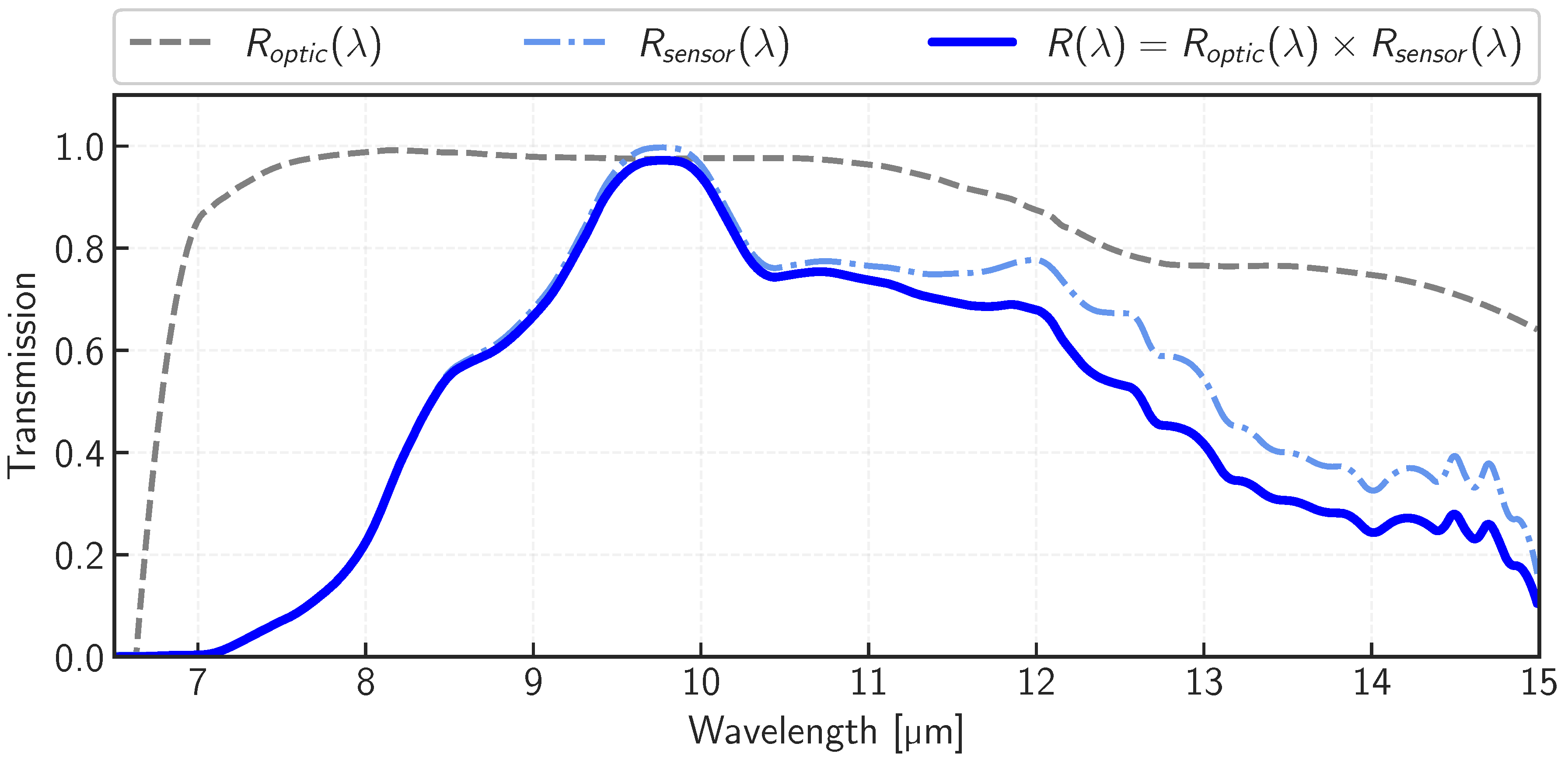
Figure 5.
Evolution of the camera NERD as a function of target temperature (blue) and equivalent scene radiance (red) assuming unity emissivity. The y-axis is common for the two curves. The green triangle depicts the NERD = 0.044 in standard operating condition. The purple reversed triangle depicts the expected NERD = 0.026 for the sample image presented in Figure 12.
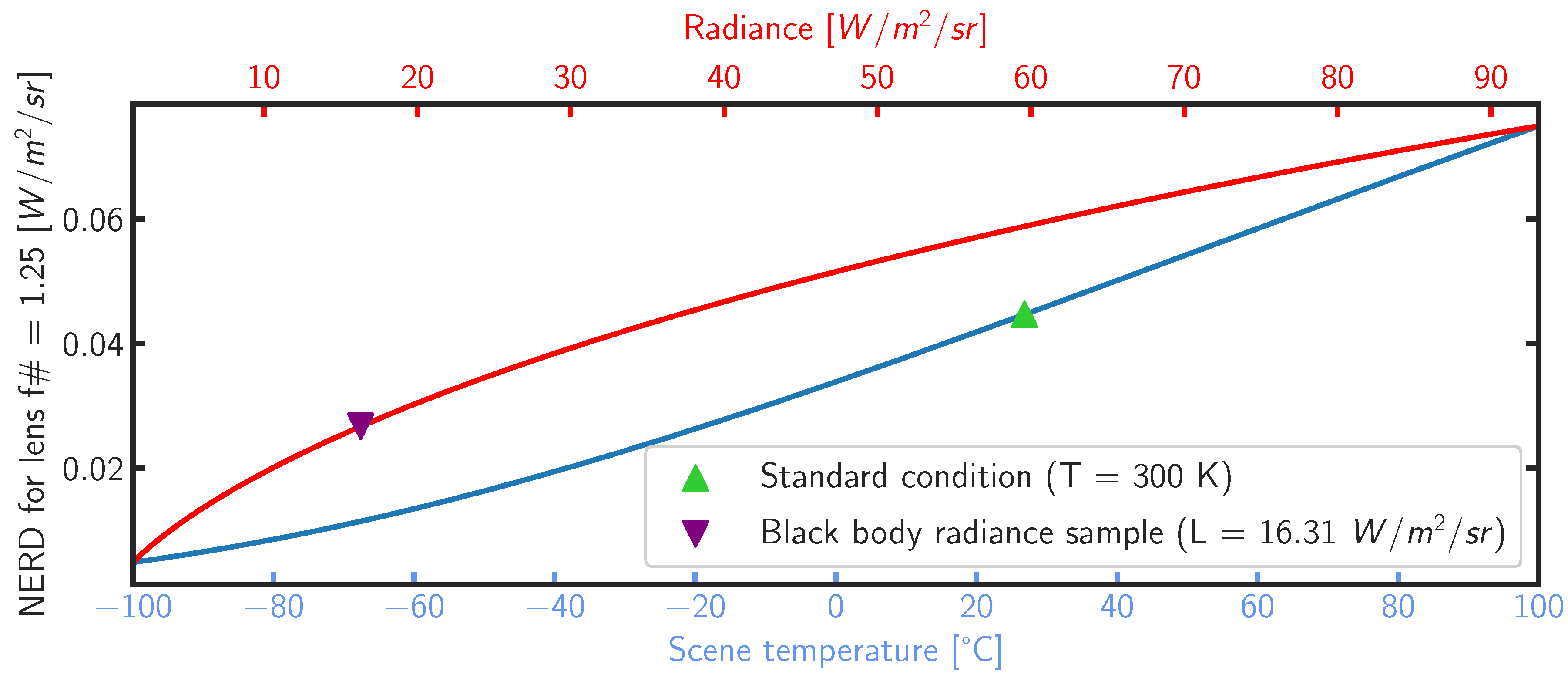
Figure 7.
Residuals for a single pixel fitted using the model described in Equation 8. Blue dots represent the model without any additional terms, while red dots indicate the fit incorporating the parameter and the difference .
Figure 7.
Residuals for a single pixel fitted using the model described in Equation 8. Blue dots represent the model without any additional terms, while red dots indicate the fit incorporating the parameter and the difference .
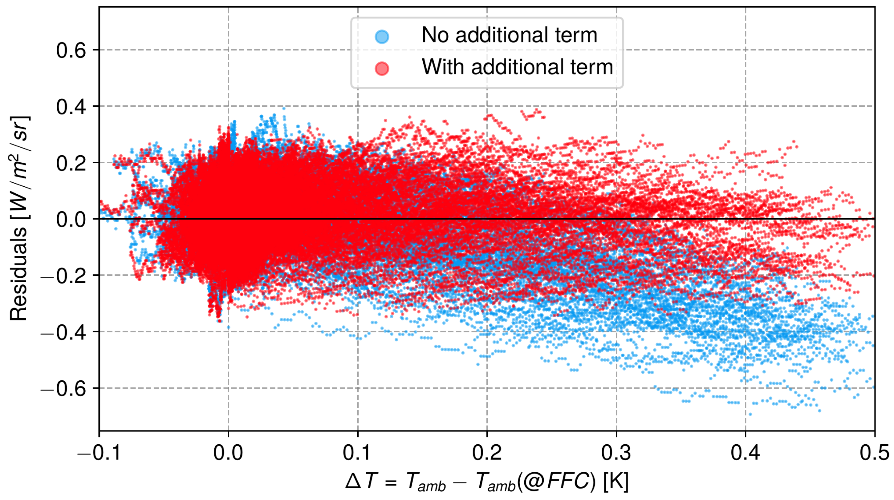
Figure 8.
Relative difference of ambient radiance contribution surrounding the blackbody source with = 0.96 against perfect blackbody = 1, during in-lab calibration experiments. As the blackbody temperature increases, the influence of ambient radiance at diminishes.
Figure 8.
Relative difference of ambient radiance contribution surrounding the blackbody source with = 0.96 against perfect blackbody = 1, during in-lab calibration experiments. As the blackbody temperature increases, the influence of ambient radiance at diminishes.
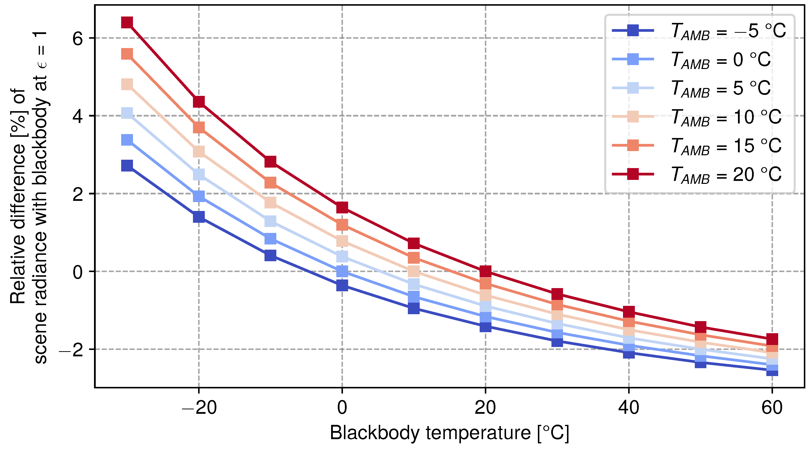
Figure 9.
Evolution of FPA temperature (dark red triangles), camera housing temperature (orange crosses), ambient/climatic chamber temperature (blue dots) for a blackbody temperature of -20°C.
Figure 9.
Evolution of FPA temperature (dark red triangles), camera housing temperature (orange crosses), ambient/climatic chamber temperature (blue dots) for a blackbody temperature of -20°C.
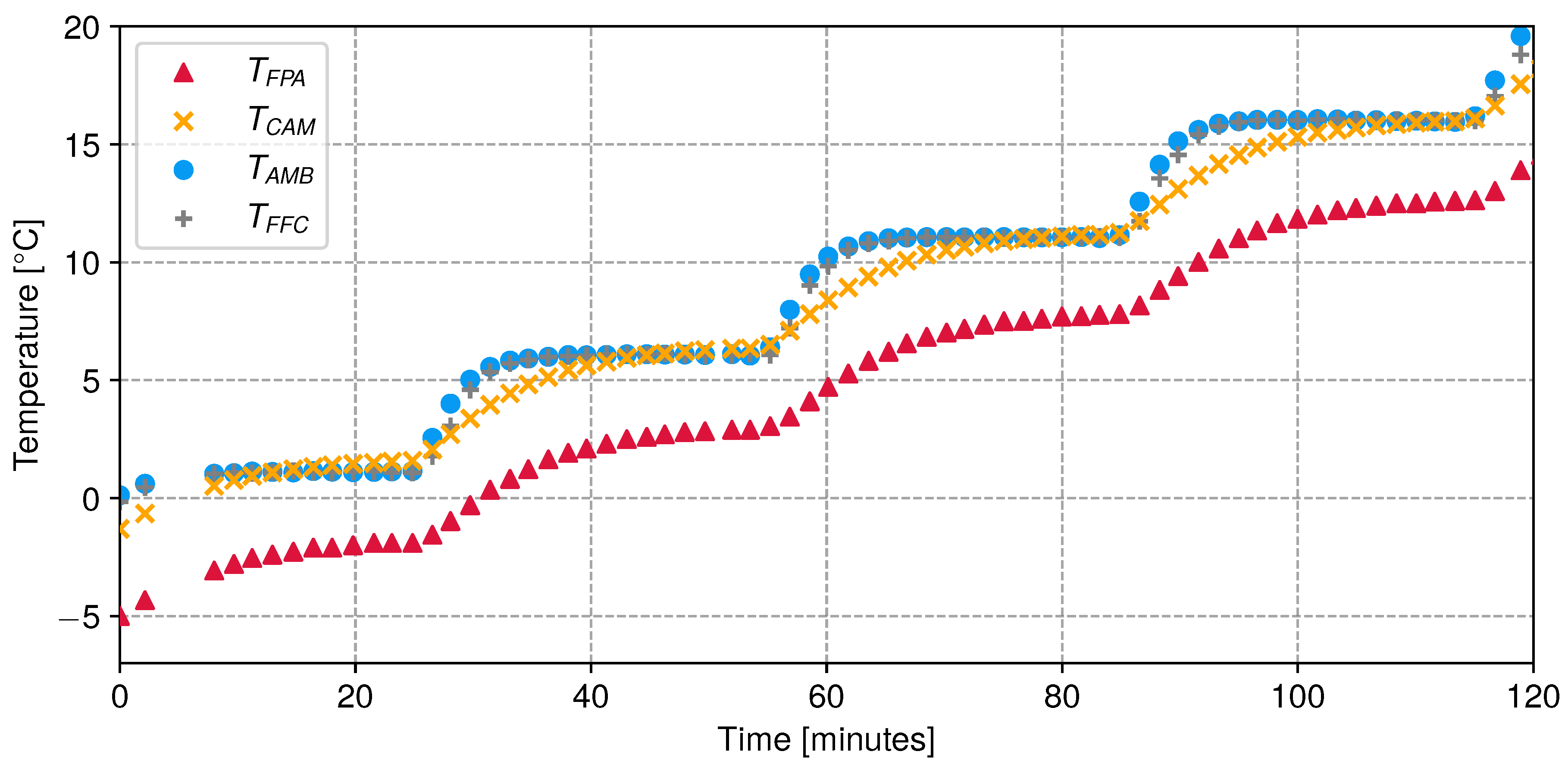
Figure 10.
(a) Sample of one blackbody image captured with default internal camera shutter support for NUC. (b) Sample of one blackbody image captured with our custom external flat-field support for NUC. Color scales are kept identical for both images. Data consists of mean subtracted raw images to only show differences in ADU. We observe a ten-times improvement in spatial uniformity by implementing our flat-field support.
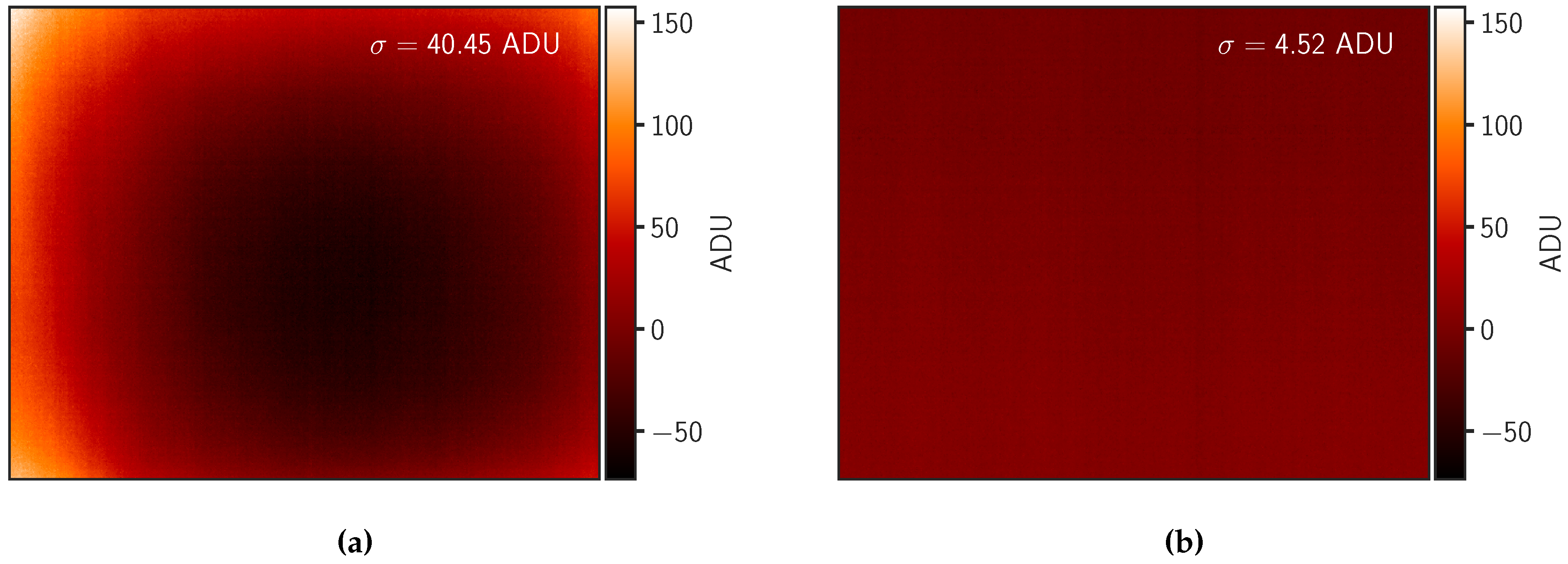
Figure 11.
Coefficient matrices reconstructed by fitting the model in Equation 14 to the calibration data. Correlations between adjacent pixels are evident for all parameters except , and a residual trace of the lens is also visible. The right column details the relative uncertainty on the fitted parameters in percent.
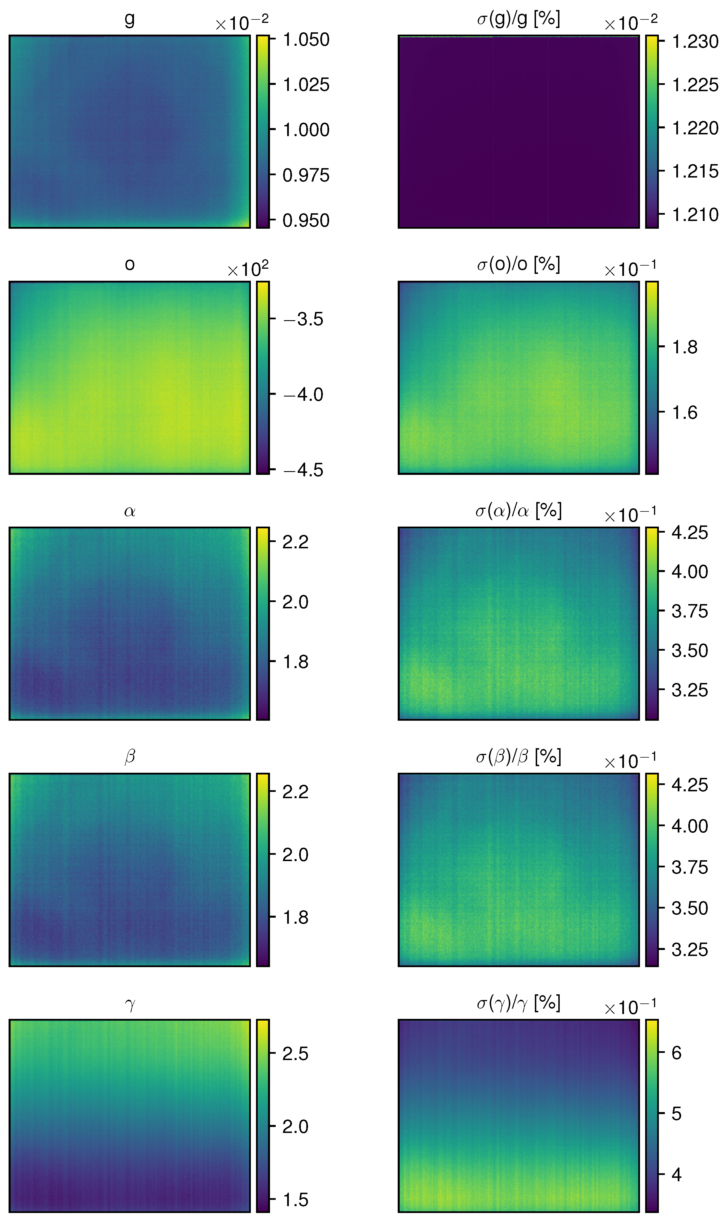
Figure 13.
(a) Simulated spectral downward radiances at zenith of Observatoire de Haute Provence, located 650 m above sea level, computed using libRadTran with a mid-latitude summer model atmosphere. Water vapor was uniformly scaled to produce a series of PWV values ranging from 0 (dark red) to 25 mm (blue) with all other atmosphere model parameters held constant: airmass = 1, air pressure = 937 hPa, total ozone column = 300 DU, no aerosol, surface temperature = 273.15 K and albedo = 0.1). Also plotted in a dashed gray line is the normalized instrument throughput curve. (b) Spectral radiances integrated over the instrument throughput as a function of PWV.
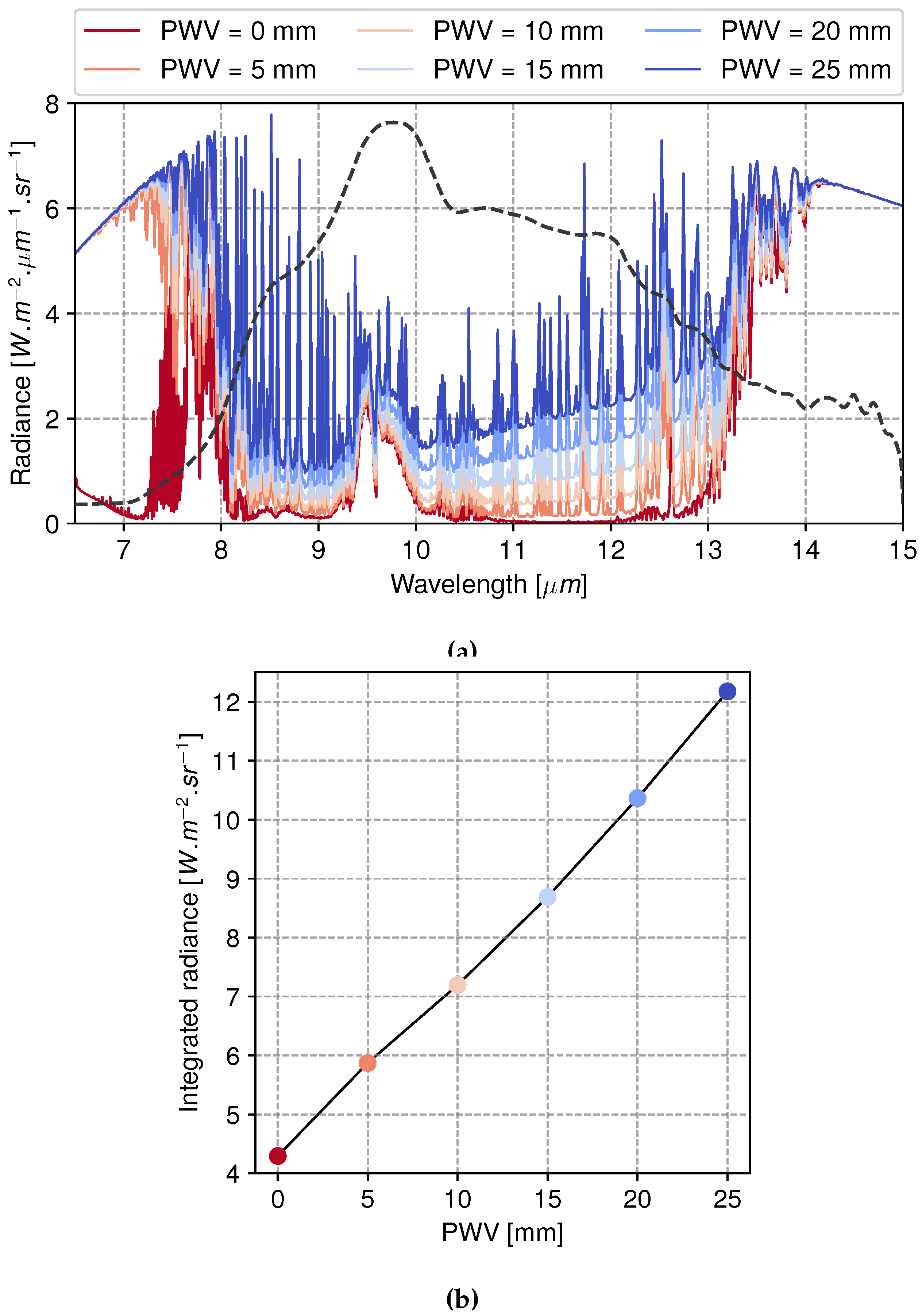
Figure 14.
(a) 13 September 2023, (b) 22 November 2023 and (c) 17 December 2023 experimental data compared to libRadTran simulations for three atmospheric profile models. The black error bars are experimental data binned over 0.02 airmass. Lower panels show the residuals between a second order polynomial fit of the calibrated data. The RMSE value is between the unbinned data relative to the fitted curve. The simulations used the PWV measured given by the ERA5 dataset and interpolated in time. Note that the simulation curves appear smooth, despite being generated for each time step (gray dots). Short time-scale variations of total ozone column, PWV, and surface temperature are too small to produce significant change in the integrated radiance.
Disclaimer/Publisher’s Note: The statements, opinions and data contained in all publications are solely those of the individual author(s) and contributor(s) and not of MDPI and/or the editor(s). MDPI and/or the editor(s) disclaim responsibility for any injury to people or property resulting from any ideas, methods, instructions or products referred to in the content. |
© 2024 by the authors. Licensee MDPI, Basel, Switzerland. This article is an open access article distributed under the terms and conditions of the Creative Commons Attribution (CC BY) license (http://creativecommons.org/licenses/by/4.0/).
Copyright: This open access article is published under a Creative Commons CC BY 4.0 license, which permit the free download, distribution, and reuse, provided that the author and preprint are cited in any reuse.


