Submitted:
09 July 2024
Posted:
10 July 2024
Read the latest preprint version here
Abstract
This study investigates the anthropogenic activities, water quality, and ichthyofaunal diversity of the Navotas Riverine Ecosystem. It examines the anthropogenic influences, analyzes the physicochemical and microbiological properties of water, identifies fish species, evaluates the water quality index, and determines ichthyofaunal diversity using various indices. Water samples and fish collections were conducted from January to April 2024 at three sites. Key findings indicate that water quality parameters such as temperature (23.20-37.5°C), dissolved oxygen (6.22-7.84 mg/L), phosphate concentration (0.55-3.72 mg/L), and fecal coliform (350-160,000 MPN/100 mL) failed to meet DENR standards for Class C water. The TDS (1153.33-10700 ppm) and conductivity (17653.33-21333.33 µS/cm) were also elevated, indicating significant pollution. The study identified low ichthyofaunal diversity, with six native and one invasive fish species. A total of 269 fish were collected: 161 from Site 1, 46 from Site 2, and 62 from Site 3. The most abundant species was Scatophagus argus (19% occurrence), while the invasive Sarotherodon melanotheron ranked third (17% occurrence). Notably, pH (r = 0.753) correlated highly with nitrate concentration. S. melanotheron significantly correlated with pH (r = 0.602, p = 0.019) and nitrates (r = 0.555, p = 0.031). Lutjanus argentimaculatus also had significant correlations with pH (r = 0.527, p = 0.039) and nitrates (r = 0.651, p = 0.011). Conversely, S. argus had a negative moderate correlation with temperature (r = -0.529, p = 0.039) and conductivity (r = -0.536, p = 0.036). These correlations suggest that the water parameters significantly influence the diversity and abundance of fish in the river. The study concludes that the river's water quality is heavily influenced by anthropogenic activities which negatively affect ichthyofaunal diversity. Recommendations include continuous monitoring, gut and heavy metal analysis of fish, assessment of avifauna diversity, and strict implementation of conservation regulations.
Keywords:
Navotas River
; Anthropogenic Activities
; Water Quality
; Ichthyofaunal Diversity
1. Introduction
Situated in Navotas, the “Fishing Capital of the Philippines,” the Navotas Riverine Ecosystem is crucially affected by both natural and anthropogenic influences. Historically, this river has supported diverse ecological communities and human livelihoods, particularly in the fishing industry. However, the river now faces significant challenges due to rapid urbanization and industrialization. Activities such as urban runoff, industrial discharge, agricultural practices, and deforestation have severely impacted the river’s health and sustainability.
Navotas, with a population of 247,543 as per the 2020 census (Philippine Statistics Authority, 2020), features a riverine system positioned between 14°40’34” N 120°56’00” E and 14°38’03” N 120°57’32” E, spanning a narrow stretch along Manila Bay's eastern coast. This ecosystem, rich in water and complex networks of rivers, bays, and estuaries, supports various aquatic species vital to local populations. Approximately 70% of Navotas’ population relies on fishing and related industries for their livelihood (Dacumos, 2012).
Human activities such as urban growth, industrial development, and population increase have led to environmental challenges including pollution, habitat loss, and changes in water quality. These issues negatively affect fish species diversity, leading to increased competition among fishermen and aquatic animals. The modern anthropogenic pressures are threatening fish biodiversity, causing eutrophication, decreased oxygen levels, and reduced habitat availability.
Fish diversity is critical for maintaining ecological balance in riverine habitats. Fish serve as biomonitors for aquatic ecosystems due to their unique biological characteristics and their dominance in most bodies of water. The study of fish biodiversity in the Navotas Riverine Ecosystem is essential for understanding the impacts of anthropogenic activities on water quality and fish variety. This research will provide baseline information necessary for the conservation and protection of the river.
2. Paper Review Summary
2.1. Navotas River System
The Navotas River, also known as the Malabon-Navotas-Tullahan River, is situated in Navotas City, Metro Manila, bordered by the Tanza River to the North, Malabon City and Estero de Maypajo of Caloocan City to the east, Manila Bay to the west, and Manila City to the south. Spanning coordinates from 14°40’34” N 120°56’00” E to 14°38’03” N 120°57.32” E, the river system comprises five major waterways draining Navotas City. It originates at the Tangos River in the city's north, with a length of approximately 6.6 kilometers and widths varying from 50 to 180 meters. Passing through 16 barangays across Navotas, Malabon, Caloocan, and Manila, the river maintains an average terrain elevation of about 2 meters above sea level. Classified by the DENR-Environmental Management Bureau (2018) as Class C water, it supports agricultural, recreational (Class II), and aquatic resource propagation uses (Figure 1).
2.2. Anthropogenic Activities
Human activities have profoundly impacted water bodies over the years, particularly rivers, through various forms of pollution. These activities include the deliberate disposal of waste materials, industrial and agricultural runoff, sewage discharge, and improper garbage management. Deforestation, urbanization, and changes in land use have exacerbated sedimentation in rivers, while practices like dam construction and overfishing have damaged aquatic habitats and threatened fish diversity. Climate change further complicates matters by altering precipitation patterns and temperatures, thereby influencing river flow and water quality. These cumulative pressures degrade water quality, harm biodiversity and ecosystems, and compromise access to clean water for human societies.
In Metro Manila, river systems such as the Marikina River, San Juan River, Paranaque River, Pasig River, and Navotas-Malabon-Tullahan River are classified as Class C water bodies, indicating moderate water quality. Despite this classification, the reliance of many local residents on fishing for livelihood makes this moderate status concerning. Informal settlements along rivers and flood-prone areas have also proliferated without proper regulation, leading to reduced drainage areas and increased flooding during heavy rainfall. The disposal of waste and uncontrolled urban expansion further contributes to the deterioration of water quality in the Navotas River and other Metro Manila rivers (Regmi, 2018).
The Navotas-Malabon River, specifically in Navotas City, suffers from significant pollution due to the absence of a comprehensive sewerage system. Although households and establishments are mandated to use septic tanks for wastewater treatment, informal settlers often bypass these regulations, contributing to river pollution and the broader health issues of Manila Bay. Efforts by Maynilad Water Services, Inc. (MWSI) to offer free septic tank desludging services aim to mitigate this problem (City Government of Navotas, 2015). Nevertheless, the Navotas-Malabon-Tullahan-Tangos River remains among the most polluted, exacerbated by solid and liquid waste discharge from industries along its banks. Domestic, commercial, and industrial wastes are often discharged directly into the river or into septic tanks and drainage canals, resulting in murky water and foul odors. Nearby landfills receive substantial daily waste deposits, further damaging marine ecosystems and mangroves within close proximity (Gan, 2017).
The complex issues facing the Navotas River system stem predominantly from anthropogenic activities, which have had widespread and detrimental effects. These activities include pollution, urbanization, habitat degradation, and unsustainable fishing practices, all of which significantly impact the ecological health of the river and the well-being of nearby communities. Similar challenges are observed in urban river systems worldwide, where human activities within riparian environments exert substantial pressures. Contaminants from residential and industrial sources pose serious threats to water quality, rendering it unfit for consumption and adversely affecting aquatic life. Urban development alters natural hydrological cycles, heightening flood risks and erosion, while habitat degradation disrupts ecosystem balance and diminishes biodiversity.
2.3. Water Quality Assessment
Water quality is a critical aspect of environmental health, impacting both human and ecosystem well-being. It encompasses various parameters, such as chemical, physical, and biological characteristics, to assess its suitability for specific purposes like drinking, swimming, or sustaining aquatic ecosystems. The measurement and assessment of water quality involves an array of factors, including the concentration of dissolved oxygen, levels of bacteria, salinity, and turbidity. Additionally, in some bodies of water, particularly in urban and agricultural areas, the presence of microscopic algae and contaminants such as pesticides, herbicides, heavy metals, and other pollutants are essential considerations (National Ocean Service, 2023).
Water quality evaluation is inherently contextual, depending on the intended use of the water. Recognizing that water suitable for drinking may not be suitable for industrial processes or recreational activities, water quality is a relative assessment aiming to match its condition with its intended purpose. Poor water quality poses health risks for both humans and ecosystems. For people, inadequate water quality can lead to a range of health issues when used for drinking, bathing, or cooking. It can also have far-reaching ecological consequences, affecting marine life in ecosystems like coral reefs and seagrass communities where clean water with low nutrient levels is essential (National Ocean Service, 2023).
2.3.1. pH
The concept of pH in water quality assessment is fundamental in understanding the acidity or alkalinity of a solution. The pH levels affect water corrosiveness and carbonate-bicarbonate equilibrium, impacted by physicochemical changes (Bhateria & Jain, 2016).
2.3.2. Temperature
Temperature significantly influences water chemistry, affecting mineral dissolution and ion concentration, crucial for aquatic ecosystems (Hamid et al., 2019; Brett, 2014).
2.3.3. Total Dissolved Solids
Total Dissolved Solids (TDS) encompass all substances in water, indicating contamination levels and affecting aquatic life (Fletcher, 2023).
2.3.4. Electrical Conductivity
Electrical conductivity (EC) reflects ion concentration, vital for assessing water pollution and ecosystem health (Ministry of Environment, 2020; Fondriest Environmental, Inc., 2014).
2.3.5. Turbidity
Turbidity affects light penetration and aquatic productivity, influenced by suspended particles like urban runoff (Fondriest Environmental, Inc., 2014; JoVE Science Education Database, 2023).
2.3.6. Dissolved Oxygen
Dissolved Oxygen (DO) levels are critical for aquatic organisms' respiration, influenced by temperature and organic matter (Floyd, 2021; Fondriest Environmental, Inc., 2013).
2.3.7. Nitrates
Nitrates from agriculture can lead to eutrophication, impacting aquatic ecosystems and human health (United States EPA, 2023).
2.3.8. Phosphates
Excessive phosphates contribute to eutrophication, reducing oxygen and harming aquatic life (United States EPA, 2023).
2.3.9. Fecal Coliform
Fecal coliform bacteria indicate sewage contamination, posing health risks in water bodies (Coliform Bacteria in Drinking Water, 2023).
2.4. Philippine Clean Water Act of 2004
The Philippine Clean Water Act (Republic Act 9275) aims to protect and manage water resources, addressing pollution from various sources (Arellano Law Foundation, 2004).
2.5. Water Quality Index
The Water Quality Index (WQI) provides a numerical assessment of water quality based on multiple parameters, aiding in monitoring and managing water resources (Caabay, 2020; Iticescu et al., 2019).
2.6. Fish Diversity
Fish represent the largest group of vertebrates, with over 31,000 species (OpenStax, 2021). Despite sharing basic immune system components with other vertebrates, fish possess unique immunological characteristics (Hsu & Du Pasquier, 2015).
The study of fish diversity in the Navotas River is particularly significant due to Navotas City's designation as the "Fishing Capital of the Philippines." Research on fish diversity and distribution provides critical data for conservation management. According to the City Government of Navotas (2015) Comprehensive Land Use Plan for 2016-2025, species such as tunsoy (Sardinella tawilis), asohos (Sillago argentifasciata), bicao (Eleutheronema tetradactylum), malakapas (Gerres erythrourus), sapsap (Leiognathus longispinis), and salinas (Alepes melanoptera) are found in the area, though their abundance and conservation status are not specified.
2.7. Diversity Index
"Biodiversity" refers to the variety of life on Earth and the interconnections between living things. High species diversity typically indicates a healthier ecosystem. Community and ecosystem diversity involves comparing different ecosystems to determine their diversity levels (Negi & Mamgain, 2013). A diversity index quantifies the variety of categories (e.g., species) within a dataset. These indices measure richness, evenness, and dominance in various contexts, often focusing on species but applicable to other classifications (Wilson & Primack, 2023). This study uses several diversity indices:
2.7.1. Species Importance Value Index
The Species Importance Value (SIV) index measures the ecological significance of a species based on its abundance, frequency, and dominance. In freshwater ecosystems, a higher SIV index indicates greater ecological importance (Libretexts, 2024).
2.7.2. Shannon-Wiener Diversity Index
The Shannon-Wiener Diversity Index estimates ecosystem species richness and abundance, useful for comparing multiple communities (Omayio & Mzungu, 2019). The Shannon-Wiener Index is denoted as H′, pi is the proportion of individuals in the ith species, and ln is the natural logarithm (Kumar, 2022). The formula of the Equation (1) is:
2.7.3. Simpson’s Diversity Index
Simpson’s Diversity Index measures species diversity by considering species number and relative abundance. Equation (2) is:
where D ranges from 0 (no diversity) to 1 (infinite diversity), n is the number of individuals in a species, and N is the total number of individuals (Nguyen, 2017; Simpson's Diversity Index, 2023). This index is widely used in ecological studies to compare biodiversity across different areas (Sharashy, 2023).
2.7.4. Margalef’s Richness Index
Margalef’s Richness Index measures species richness, frequently used to compare the diversity of ecological communities. Equation (3) is:
where S refers to the total number of species, N refers to the total number of individuals in the sample, and ln is the natural logarithm (Ozkan et al., 2024). Higher values indicate greater species richness.
2.7.5. Sorensen’s Coefficient Similarity Index
Sorensen’s Coefficient Similarity Index assesses species similarity between two communities. Equation (4) is:
It is calculated by analyzing the degree of similarity of species between two communities, where A refers to the number of unique species in Community A, B refers to the number of unique species in Community B, and C refers to the number of shared species in Community A and B (Rahman et al., 2019).
2.7.6. Shannon’s Equitability
The Shannon Equitability Index measures how evenly distributed the species are within a population. Equation (5) is:
where H refers to the Shannon Diversity Index and S refers to the total number of unique species present. The Shannon Equitability Index has a value ranging from 0 to 1, with 1 indicating complete evenness (Bobbitt, 2021).
3. Methodology
3.1. Study Area
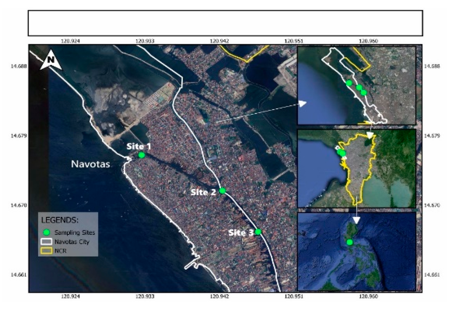
The study area is shown in Figure 2. The study of the Navotas-Malabon-Tullahan (NMT) Riverine System spanned from January to April 2024. Three sites were selected:
- Site 1: 14°40’35” N, 120°55’57” E, estuary near Manila Bay, populated by fishermen.
- Site 2: 14°40’19” N, 120°56’33” E, diverting channel of Tanza and Tangos Rivers.
- Site 3: 14°39’60” N, 120°56’48” E, downstream leading to Tullahan River.
Distances:
- Site 1 to Site 2: 1.18 km
- Site 2 to Site 3: 0.80 km
Figure 2.
Map of NMT River System with Three Sampling Sites Indicated.
3.2. Administration of Structured Questionnaire
A survey with 782 respondents was conducted, covering demographics, anthropogenic activities, and river conservation efforts. Responses were measured on a Likert Scale. Key informant interviews were also conducted with fishermen to understand fishing practices and harvests.
3.3. Water Sample Collection
Water samples were collected monthly using grab sampling from 9 to 10 a.m. Parameters measured included pH, temperature, conductivity, TDS, dissolved oxygen, turbidity, phosphates, nitrates, and fecal coliforms.
3.3.1. Water Quality Parameters
- pH and Temperature: Digital pH Pen Meter and laboratory thermometer.
- Conductivity and TDS: Digital Multi-function LCD Monitor.
- Turbidity: Modified Secchi Disk.
- Dissolved Oxygen: DO9100 Dissolved Oxygen Meter.
- Nitrates: Tested using 352.1 Brucine – Colorimetric Method.
- Phosphates: Tested using Hitachi UH5300 UV-Vis Spectrophotometer.
- Fecal Coliforms: Tested using 9221 E. Multiple Tube Fermentation Technique
3.4. Determination of Water Quality
Water quality was assessed using the Weighted Arithmetic-Water Quality Index (WA-WQI), which considers multiple parameters and their respective weights to calculate an overall index.
3.5. Collection of Fish Samples
Fish samples were collected by fishermen using cast nets and basket traps, then identified and verified by experts.
3.6. Computation of Diversity Index
Several indices were used to analyze fish diversity:
- Species Importance Value (SIV): Dominance of species.
- Shannon-Wiener Index (H'): Species diversity.
- Simpson’s Diversity Index (D): Species diversity.
- Margalef’s Richness Index (R): Species richness.
- Sorensen’s Coefficient (IS): Community similarity.
- Shannon’s Equitability (EH): Species evenness.
3.7. Statistical Treatment of Data
- Kruskal-Wallis Test: Differences in water quality among sites.
- Friedman Test: Differences in water quality over time.
- Pearson R Correlation: Relationships among water quality parameters and between water quality and fish species.
4. Results and Discussion
4.1. Anthropogenic Activities in the Navotas River
A survey questionnaire was administered along with consent interviews to 782 respondents. The results indicated that most respondents were male, comprising 78.6% of the population, while female respondents made up 21.4%. Among the respondents, 71.4% were high school graduates. The marital status was evenly split, with 50% being single and 50% married. The age distribution was as follows: 14.3% were aged 18-27, 21.4% were aged 28-37, 50% were aged 38-47, and 14.3% were aged 48 and above. Respondents belonged to families with 2-4 members (42.9%), 5-7 members (50%), and 8-10 members (7.1%). In terms of occupation, the respondents included fish net weavers (11.51%), fishermen (78.6%), sari-sari store owners (6.39%), and vendors (3.45%). Table 1 below presents the survey results of anthropogenic activities in the Navotas River.
Table 1 illustrates the anthropogenic activities occurring in the Navotas River. It shows that fishing and boating were common activities in the river. However, respondents claimed that due to the poor water quality at the time, their fish catch had decreased significantly. The survey indicated that activities such as washing clothes, discharging wastewater from laundry, and disposing of untreated household wastewater occurred infrequently. In contrast, activities like irrigating plants with river water, excreting domestic waste, throwing garbage into the river, and practicing aquaculture were never practiced in the river. Respondents mentioned that they used to practice aquaculture, but urban development of industries and commercial sectors led to the purchase of a large area of the river, halting their ability to farm fish and shrimp.
Additionally, they reported having a dumping site located in Barangay Tanza, with garbage collected weekly by waste collectors. However, although the mean score for throwing garbage into the Navotas River is low (x̄ = 1.07) based on the observations during the survey, most of the visible waste in the river was non-biodegradable. This included PET bottles, single-use plastics, plastic food wrappers, Styrofoam, and medical wastes, which are harmful to various species inhabiting the river. These wastes and floating debris came from upstream sources, including the Taliptip River, Sta. Maria River, and Meycauayan River, flowing through the Tanza River (Malabon, Navotas Spared Due to Flood Mitigation Measures: Ang, 2020). Furthermore, these rivers transport waste from commercial establishments, manufacturing industries, households, hospitals, and other facilities that find their way into the Navotas River before it flows out to the Manila Bay.
Based on the interviews, residents admitted having inadequate sanitation. They lacked proper pipelines, such as sewers, drainage pipes, and wastewater pipes. In some cases, the wastewater from their households was directly discharged into the river, as reported by 71.40% of the respondents. Furthermore, during the survey at Navotas River, researchers observed various pollutants. The water had a distinct color and unpleasant odor, ranging from murky brown to greenish hues. Floating debris, including plastic bottles, bags, and other garbage coming from nearby industries, was abundant and created clusters of waste along the river. Industrial runoff was also observed in the river, characterized by an oil sheen on the surface of the water, particularly near the discharge points. Sewage contamination was visible from raw sewage outlets and the presence of fecal matter in some parts of the river.
These field observations justify that the Navotas River is heavily polluted and heavily impacted by different anthropogenic activities.
4.2. Water Quality of Navotas River during the Four-Month Period
The Navotas River, shaped by the high tides and strong currents from Manila Bay, is an essential aquatic habitat in northern Navotas City, providing breeding grounds for various ichthyofaunal species. However, the aquatic resources in the river, particularly fish, are under severe fishing pressure and suffer from deteriorating water quality.
Table 2 presents the physicochemical and microbiological properties of water samples collected from three distinct sites in the Navotas River from January to April 2024. Water quality parameters were compared to the standards set by DENR Administrative Order No. 2016-08 for Class C waters, with fecal coliform and phosphate concentrations compared to the amendment order DENR Administrative Order No. 2021-19.
4.2.1. pH
The pH levels of the water in the Navotas River were found to be compliant with the DENR standard value for Class C water at all sites across the four-month sampling period, as measured using a Digital pH Pen Meter. Figure 3 illustrates the pH levels of the water in three sampling sites during the sampling periods from January to April 2024.
The average pH levels of the water from January to April 2024 were 7.52, 7.07, 6.89, and 7.04, respectively. The pH values acquired from the January, February, and April sampling were slightly basic, while the pH value from the March sampling was slightly acidic. The presence of impurities such as sodium carbonate, potassium bicarbonate, or potassium carbonate influenced the basicity or alkalinity of the water. In contrast, the acidity of the water was attributed to the presence of acidic compounds such as nitrogen compounds. Additionally, the decomposition of dead fish and plants emitted ammonia and other carbon dioxide, lowering the pH of the water and making it more acidic.
The pH levels recorded among the three sampling sites during monthly water sampling from January to April 2024 showed notable variations. Site 1, located at the estuary of Tangos River, consistently exhibited the highest pH level across all sampling months. In contrast, Site 2 recorded the lowest pH level for January, February, and April, but surprisingly exhibited the second-highest pH level in March. Site 3 showed the second-highest pH levels for January, February, and April, but notably had the lowest pH level in March.
The decline in pH level during March may have been attributed to the increasing heat island effect, which caused an increase in biological activity within the river, such as the growth of algae and bacteria (Vergara & Blanco, 2023). Construction projects near the river could have contributed to the decline in the pH level of the water in Navotas River during March 2024. Moreover, human activities, such as the discharge of heated effluents from industrial processes, could have contributed to thermal pollution in rivers. The elevated water temperatures from thermal pollution can directly influence pH levels by affecting chemical equilibria and biological processes.
4.2.2. Temperature
Water temperature plays a crucial role in influencing various physical and chemical properties. Figure 4 depicts temperature variations at three sampling sites over the four-month period.
The average temperature of the water from January to April 2024 were 25.23 °C, 28.44 °C, 28.76 °C, 35.89 °C respectively. Given the data presented above, it can be clearly seen that the values exceed even the highest limit for Class C water according to DENR DAO 2016-08 particularly in the month of April. All sampling sites exhibited high temperature in April.
4.2.3. Total Dissolved Solids
TDS levels, indicative of dissolved mineral content, were measured across the river. Figure 5 illustrates TDS variations during the sampling period.
The average TDS concentrations recorded during sampling periods were 9611.08 mg/L (Site 1), 7626.67 mg/L (Site 2), and 7425.83 mg/L (Site 3). The results indicated that Site 1 had the highest mean TDS value of 9611.08 mg/L, suggesting significant sources of dissolved minerals and salts at this site. Site 2, with an average of 7626.67 mg/L, had a moderate level of dissolved solids. Site 3 recorded the lowest TDS concentration at 7425.83 mg/L, suggesting less anthropogenic influence in the area.
The consistently high TDS concentrations at Site 1 indicate possible pollution sources affecting the water quality in the Navotas River. Both excessively high and low concentrations of TDS can inhibit the growth and potentially lead to the death of many aquatic organisms. Elevated TDS levels can reduce water clarity and raise water temperatures, impacting the overall health of the aquatic ecosystem.
4.2.4. Electrical Conductivity
EC measurements reflect water's ability to conduct electricity, influenced by dissolved ions. Figure 6 presents EC levels across the sampling sites.
The average conductivity of the water from January to April 2024 were 18647.78 µS/cm, 18910.00 µS/cm, 19466.67 µS/cm, and 20311.11 µS/cm respectively. For Site 1, the electrical conductivity (EC) levels exhibited a moderate decrease in February, followed by a constant increase in March and April. This trend indicates an increased concentration of dissolved ions in the water over time. At Site 2, there was a subtle increase in EC levels from January to February, a moderate decrease in March, and an increase in April. This pattern suggests that ion concentrations are generally rising. At Site 3, EC levels were substantial with minor changes, peaking in February and moderately decreasing towards April, indicating that ion concentration is relatively stable with minor fluctuations.
The increased EC levels at Site 1, particularly in April, suggest an inflow of dissolved ions, likely due to increased runoff. This implies that water quality at this site is unfavorable concerning salinity.
4.2.5. Turbidity
Turbidity, caused by suspended particles, affects water clarity and light penetration. Figure 7 displays turbidity levels recorded during the study period.
The observed data from Navotas River at three sampling sites over four months presented interesting variations. In January, the values were 89.67 cm at Site 1, 88.67 cm at Site 2, and the highest at 117.33 cm at Site 3, indicating better conditions or higher fish activity at Site 3 compared to Sites 1 and 2. In February, Site 2 recorded the highest value at 101.67 cm, suggesting peak conditions at this site, with Site 1 and Site 3 showing slightly lower values at 91.67 cm and 95.67 cm, respectively. March showed a significant peak at Site 2 with 135 cm, while Sites 1 and 3 had lower values of 80 cm and 84 cm, respectively, indicating a possible seasonal effect or specific event contributing to the high activity at Site 2. In April, Site 1 had the highest observed value at 100 cm, followed by Site 2 at 95 cm and Site 3 at 88.33 cm, suggesting a shift in favorable conditions towards Site 1.
The average observed values per site across all months were 90.34 cm for Site 1, 105.34 cm for Site 2, 96.83 cm for Site 3. This indicates that Site 2 generally had the highest observed values, followed by Site 3 and Site 1. On a monthly basis, the average observed values were 98.56 cm in January, 96.33 cm in February, 99.67 cm in March, and 94.44 cm for April. These averages show relatively consistent levels of activity or conditions throughout the months, with March having the highest average and April the lowest.
4.2.6. Dissolved Oxygen
DO levels, crucial for aquatic life, were monitored throughout the river. Figure 8 illustrates DO variations across the sampling sites.
The concentration of dissolved oxygen (DO) in the Navotas River was measured using the digital DO Meter. The concentration of DO in the river ranged from 6.22 to 7.84 mg/L. The average DO level of water recorded from January to April were 6.52 mg/L, 6.96 mg/L, 7.71 mg/L, and 6.78 mg/L respectively. The DO level in March did not meet the acceptable standards set by the DENR for Class C waters. This can be attributed to the high level of organic waste in the river due to the improper sewage system in the area. Organic materials found in sewage from homes and industries are broken down by microbes, which need oxygen in the process. The variation of DO concentrations among sampling months can be attributed to the changing weather conditions, salinity, total coliform, and other factors.
4.2.7. Nitrates
Nitrates, essential nutrients but indicators of pollution, were measured. Figure 9 shows nitrate concentrations across the sites.
The average nitrate levels for each site were 0.27 mg/L (Site 1), 0.28 mg/L (Site 2), 0.28 mg/L (Site 3) respectively. These concentrations were within the standard set by DENR for Class C waters. For Site 1, January and April had the highest level of nitrates among all the months and sites. Site 2 and 3 both showed generally lower nitrate concentrations with the lowest result in the month of April. Site 1 consistently showed higher concentrations compared to site 2 and 3. This suggests that the surveyed areas of the Navotas Riverine Ecosystem are affected by anthropogenic activities which can be the cause of presence of nitrates in each of the sites. While the nitrate concentration is typically low in Navotas River, it can possibly become elevated due to industrial waste, refuse dump runoff, or human and animal waste contamination.
4.2.8. Phosphates
Phosphate concentrations, indicative of nutrient pollution, were assessed. Figure 10 presents phosphate levels across the river.
The phosphate concentration observed from three sites along Navotas River reveals varying levels across different months. Site 1 consistently exhibited higher phosphate concentrations compared to Sites 2 and 3, with average values of 2.47 ppm, 2.16 ppm, and 1.74 ppm, respectively.
The elevated levels at Site 1, averaging 2.47 ppm, suggest significant anthropogenic influences, potentially due to industrial discharge, agricultural runoff, or domestic sewage inputs into the river. Site 2, with an average phosphate concentration of 2.41 ppm, displays fluctuating levels, possibly influenced by seasonal changes, weather patterns, and upstream activities such as heavy runoff or agricultural practices. Conversely, Site 3 consistently showed the lowest phosphate levels, with an average of 1.18 ppm, indicating either minimal upstream phosphate sources or effective natural or man-made processes mitigating inputs. Despite these variations, all sites underscore the importance of effective management strategies to control phosphate pollution and preserve the health of Navotas River's aquatic ecosystem, as even low levels of phosphates can contribute to eutrophication over time when combined with other nutrients like nitrogen.
Phosphates in the Navotas River originate from natural sources, including the release of phosphorus from bed sediments and the breakdown of organic phosphorus compounds by bacteria. These organic compounds are primarily generated by biological systems and are present in debris such as plant waste. Additionally, anthropogenic activities contribute to phosphate levels in the river, with organic phosphates from household food, body waste, and natural animal manure entering the water supply through sewage and wastewater systems. Common household detergents have emerged as a modern source of phosphorus in aquatic bodies, entering wastewater systems and ultimately releasing into surface waters, resulting in elevated phosphate levels.
4.2.9. Fecal Coliform
Fecal coliform levels, indicating contamination from human and animal waste, were monitored. Figure 11 illustrates fecal coliform concentrations across sampling sites.
At Site 1, a notable increase was observed from January to February, reaching a peak of 160,000 MPN/100mL. Subsequently, in March, a decrease was noted, followed by a further decrease in April. Conversely, at Site 2, a persistent increase was seen from January to March, reaching 160,000 MPN/100mL in March. However, April showed a sudden decrease, albeit remaining at a high level, indicating continuous contamination. The sudden decrease in fecal coliform level in the Site 1 from March to April 2024 may be attributed by the increased temperature in April (34.5 °C) leading to the natural die-off coliform bacteria over time due to increased UV radiation. Site 3 exhibited a consistently high level from January to February and April, with a slight decrease in March, suggesting extreme contamination in this area.
The significant differences in terms of fecal coliform levels in the sampling months (temporal variations) across all sites may be attributed by the seasonal changes during the dry season, particularly on January and February, when the river experience low tide resulting in higher concentration of contaminants due to reduced dilution (X ̅February = 137333.33 MPN/100 mL and X ̅January = 95666.67 MPN/100 mL).
The significant differences in fecal coliform levels among the sampling sites (spatial variations) across the sampling months may be attributed by the site-specific variations whereas sites near the urban areas or industrial zones (Site 2 and Site 3) have consistently higher fecal coliform levels (X ̅Site 2 = 94750 MPN/100 mL X ̅Site 3 = 143000 MPN/100 mL). Overall, all three sites of Navotas River show contamination based on their fecal coliform levels. The frequent occurrence of high levels, particularly reaching 160,000 MPN/100mL, exceeds acceptable thresholds, posing potential health risks to locals exposed to it.
4.3. Kruskal-Wallis Test
The Kruskal-Wallis Test was employed to determine if there were significant differences in the water parameters measured among the sampling sites during the sampling periods from January to April 2024. The results of the Kruskal-Wallis Test conducted to assess the statistical significance of variations in water quality parameters across the sampling sites over four sampling months are presented in Table 3.
The Kruskal-Wallis Test Results presented in Table 3 revealed significant and non-significant differences in water quality parameters among the sampling sites per sampling month, highlighting the impact of anthropogenic activities on the Navotas Riverine Ecosystem.
- pH: Significant variations were observed in February, March, and April (p-value = 0.027), while January (p-value = 0.925) showed no significant difference. This indicates changes in water chemistry likely influenced by pollution sources or natural processes, with stability in January possibly due to balanced buffering capacity or reduced pollutant input.
- Temperature: Displayed significant changes in February (p-value = 0.026), March (p-value = 0.020), and April (p-value = 0.021), while January (p-value = 0.058) was non-significant. These fluctuations could be attributed to seasonal warming and increased industrial or domestic discharges, impacting aquatic life and ecosystem health.
- Total Dissolved Solids (TDS): Showed non-significant differences in January (p-value = 0.575), February (p-value = 0.065), and March (p-value = 0.517), with a significant difference in April (p-value = 0.027). This suggests relatively stable dissolved solid levels, indicating consistent water quality regarding mineral content, with potential pollution events in April.
- Electrical Conductivity (EC): Was non-significant in January (p-value = 0.924), February (p-value = 0.190), and March (p-value = 0.295), but significant in April (p-value = 0.035). This reflects stability in ionic concentrations, with variations in April possibly due to increased pollutant inputs.
- Turbidity: Was significant in February (p-value = 0.026), indicating increased sediment or runoff disturbance, but non-significant in January (p-value = 0.066), March (p-value = 0.066), and April (p-value = 0.148), suggesting minimal disturbance or effective sediment settling. The water in Navotas River was turbid, containing a higher concentration of suspended particles, including clay, silt, fine organic and inorganic materials, soluble colored organic compounds, and other microscopic organisms.
- Dissolved Oxygen (DO): Exhibited significant differences in January, February, and April (p-value = 0.027), but was non-significant in March (p-value = 0.295). These variations reflected changes in temperature, organic load, or water flow, impacting aquatic life.
- Nitrates: Consistently showed significant variations across all months (p-value = 0.018). The consistent significance in nitrate levels pointed to ongoing nitrate pollution, likely from agricultural runoff or sewage discharge, which could lead to eutrophication and affect water quality.
- Phosphates: Were non-significant in January (p-value = 0.066), February (p-value = 0.050), and March (p-value = 0.061), suggesting stable levels initially but increased pollution in April.
- Fecal Coliform: Consistently exhibited significant differences across all months (p-value = 0.018), indicating continuous contamination from human or animal waste, highlighting poor sanitation or waste management practices.
4.4. Friedman Test
The Friedman Test was employed to determine if there were significant differences in the water parameters measured among four sampling months for each sampling site. Table 4 presents the results of the Friedman Test for the three sampling sites within Navotas Riverine Ecosystem.
The Friedman Test Results during the sampling periods presented in Table 4 revealed significant and non-significant differences in water quality parameters among the sampling months per sampling site.
- pH: The water collected over four months showed significantly different pH levels at each site. Variations in pH levels among the sampling sites indicate potential differences in acidity or alkalinity, influenced by factors such as agricultural runoff, industrial discharge, or natural processes. Variations in pH can have significant implications for aquatic life and ecosystem health, as they directly affect the solubility of nutrients and the availability of toxic substances.
- Temperature: The test revealed significant differences in temperature across all sites, indicating statistically significant variations at each site. Monitoring temperature is important when evaluating water quality. Significant differences in temperature suggest varying thermal conditions across the sampling sites, influencing biological processes, metabolism rates, growth patterns, and reproductive behaviors of aquatic organisms. Variations in temperature also affect water chemistry and dissolved oxygen levels, impacting overall ecosystem dynamics.
- Total Dissolved Solids (TDS): Significant differences were found at Site 1 and Site 2, but not at Site 3. The lack of significant differences in TDS levels implies relatively uniform concentrations of dissolved solids across the sampling sites. While TDS levels indicate overall water quality, their non-significance at Site 3 suggests that factors influencing TDS, such as mineral content or salinity, may not have varied significantly among the sites during the sampling periods.
- Electrical Conductivity (EC): Significant differences were found only at Site 1. Like TDS, non-significant differences in EC levels at the other sites suggest consistent conductivity across the sampling sites. EC is often used as a proxy for TDS and provides insights into water quality and ion concentrations. The uniformity in EC levels indicates potential stability in ion concentrations and overall water chemistry among the sites.
- Turbidity: Significant differences were found only at Site 3. This site is near construction and ship repair activities on the riverside of Navotas River. Human activities that promote dynamic turbidity over time contribute to the murkiness of water.
- Dissolved Oxygen (DO): Significant differences were found across all sites. Variations in DO concentrations among sampling months could be attributed to changing weather conditions, salinity, total coliform, etc. DO is critical for the survival of aquatic organisms, and deviations from optimal levels indicate pollution, organic matter decomposition, or eutrophication. Monitoring DO levels is crucial for assessing water quality and ecosystem health.
- Nitrates and Phosphates: Both parameters showed significant differences in concentrations across sampling months at each site. These significant differences underscore variations in nutrient concentrations among the sampling sites. Excessive nutrient inputs, often from agricultural runoff or wastewater discharge, can lead to eutrophication, algal blooms, and oxygen depletion. Managing nutrient pollution is essential for maintaining water quality and preventing ecological degradation.
- Fecal Coliform: Significant differences were found across sampling sites, indicating varying levels of bacterial contamination. Elevated fecal coliform levels pose risks to human health and indicate sewage contamination or inadequate sanitation practices. Significant variations were observed in February, March, and April (p-value = 0.027), while January (p-value = 0.925) showed no significant difference. This indicates changes in water chemistry likely influenced by pollution sources or natural processes, with stability in January possibly due to balanced buffering capacity or reduced pollutant input.
4.5. Water Quality Index of Navotas River during the Sampling Periods
The water quality index was used to analyze the water quality in Navotas River based on various parameters such as pH, temperature, total dissolved solids, conductivity, nutrient content, dissolved oxygen, and biological oxygen demand. It simplifies complex water quality data into a single value for easy understanding. The overall water quality index of Navotas River, including the index for each site during the four sampling periods from January to April 2024, is presented in Table 5.
Based on the water quality index of the sampling months, January (WQI = 517), February (WQI = 582), March (WQI = 701), and April (WQI = 617), Navotas River is unfit or deteriorated. This is because Navotas River failed to attain the allowable limit set by the DENR for Class C water. The unfit/deterioration interpretation of the water quality of Navotas River stems from various pollutants present in the water. Navotas River faces significant pollution challenges due to discharges from industries along riverbanks, untreated or poorly treated sewage from household and commercial establishments, and stormwater runoff from streets, roads, and other impervious surfaces which carry solid waste and other debris into the river. Moreover, deforestation and removal of mangroves reduce the river’s ability to naturally filter pollutants and stabilize its riverbanks, which exacerbates erosion and sedimentation.
4.6. Ichthyofaunal Diversity of Navotas River
The present study identified fish species in Navotas River belonging to the class Actinopterygii and five families: Scatophagidae, Dorosomatidae, Terapontidae, Lutjanidae, and Cichlidae. The distribution of ichthyofauna in three sites during the sampling periods from January to April 2024 is shown in Table 6.
A total of 269 fish were collected and identified. The species with the highest total occurrence was Scatophagus argus (18.59%), followed by Pelates quadrilineatus (18.22%).
- Scatophagus argus (Linnaeus 1766), belonging to the family Scatophagidae, was the most abundant species. Known as spotted scat, it inhabits brackish estuaries and lower reaches of freshwater streams, frequently occurring among mangroves (Froese & Pauly, 2017; Randall, 2019). Scatophagus argus exhibits a wide salinity tolerance range and can survive in conditions ranging from freshwater to highly saline environments. It can tolerate elevated temperatures and low dissolved oxygen concentrations (Gupta, 2016).
- Pelates quadrilineatus (Bloch 1790), locally known as babanse, was the second most abundant species (18.22%). Found in brackish waters, this species often inhabits estuaries, seagrass beds, and mangrove bays, feeding on small fishes and invertebrates (Ching, 2023).
- Other species with lower abundances included Sarotherodon melanotheron (gloria tilapia) (17.10%), Terapon jarbua (bagaong) (15.61%), Lutjanus argentimaculatus (alakaak) (12.64%), Lutjanus argentimaculatus (kabang) (9.67%), and Nematalosa nasus (kabase) (8.18%). These species are commonly found in brackish waters, but their lower abundance may be due to seasonal variations, spawning environment differences, and tolerance for water quality changes.
- Sarotherodon melanotheron, an introduced invasive species, had the third-highest total occurrence. Its abundance can negatively impact native species by preying on their eggs and juveniles, contributing to the decline of native fish populations (Oluwale & Ugwumba, 2022).
The ichthyofaunal diversity of Navotas River reflects the varying ecological conditions and impacts of anthropogenic activities on the aquatic ecosystem. The presence of both native and invasive species indicates the complexity of biotic interactions and the influence of environmental factors on fish communities. The study highlights the importance of continuous monitoring and management to preserve the ecological balance and biodiversity of Navotas River.
4.6.1. Species Importance Value
The Species Importance Value (SIV) index measures species dominance within a specific area, determined as the sum of relative frequency, relative dominance, and relative density (Ismail et al., 2017). Table 7 shows the Species Importance Value of ichthyofaunal species, highlighting the most and least important species in the Navotas River.
Scatophagus argus (kitang) holds the highest importance value (53.84), followed by Pelates quadrilineatus (babanse) with an importance value of 51.02. The invasive Sarotherodon melanotheron has the third-highest importance value (50.87). Conversely, Nematalosa nasus (kabase) has the lowest importance value (26.76).
The abundance of S. argus indicates its dominance in the river, attributed to its resilience to environmental stressors like water pollution. Its omnivorous diet allows it to adapt to a degraded environment, feeding on detritus, algae, small invertebrates, and plant matter. Additionally, S. argus has a high reproductive rate and reaches maturity quickly, maintaining its population regardless of conditions.
Conversely, N. nasus, with the lowest importance value, demonstrates a preference for conditions less suitable to the polluted environment of the river, such as lower DO and high pollutant levels, which are disadvantageous compared to species like S. argus.
The distribution of fish species in the Navotas River provides insights into the river's health and species diversity. Identifying the pattern of species richness and the distribution of dominant species, such as S. argus, serves as an effective biomarker of the river’s condition and the impact of pollution on fish. Analyzing these patterns highlights how environmental stressors influence biodiversity and sustainability of aquatic life in the Navotas River. Table 8 shows the biodiversity status of collected fish species in Navotas River.
Among the collected species, only Pelates quadrilineatus is listed as "Not Evaluated," while the remaining six species are categorized as "Least Concern." Six species are native, while Sarotherodon melanotheron (Gloria Tilapia) is introduced.
4.6.2. Species Diversity of Ichthyofauna in Navotas River
Biodiversity indices, including the Shannon-Wiener Index, Simpson’s Diversity Index, and Margalef’s Richness Index, were used to assess the diversity and similarity of ichthyofaunal species in the Navotas River system. Presented in Table 9 were the values obtained from computed species diversity indices.
The Shannon-Wiener Index revealed that Site 1 had the highest diversity (H’ = 1.91), followed by Site 2 (H’ = 1.87). Site 3 had the lowest diversity (H’ = 1.71). According to the "Classification Scheme of Shannon-Wiener Diversity Index" by Fernando et al. (1998), an index value ≤ 1.99 indicates low species diversity. The Simpson’s Index of Diversity (1-D) indicated that Site 1 and Site 2 had relatively high diversity values (0.85 and 0.86, respectively), compared to Site 3 (0.82). The Reciprocal (1/D) of Simpson’s Diversity Index showed that Site 2 had the highest diversity (1/D = 7.04), followed by Site 1 (1/D = 6.81), and Site 3 (1/D = 5.48). Margalef’s Richness Index revealed that Site 2 had the highest richness (dmg = 1.57), followed by Site 3 (dmg = 1.45), and Site 1 (dmg = 1.18), indicating Site 1 had the lowest species richness.
Overall, Navotas River had low diversity (SDI ≈ 0.99), likely due to anthropogenic activities such as pollution and the proliferation of invasive species like Gloria Tilapia (S. melanotheron), which compete for food sources and prey on smaller organisms.
4.6.3. Species Similarity and Species Evenness in Navotas River
Understanding fish species' biodiversity and distribution in Navotas River is crucial for conservation efforts and monitoring ecosystem health. Sorensen’s Coefficient Similarity Index quantifies the similarity between communities, and Shannon Equitability measures species abundance evenness. Presented in Table 10 and Table 11 were the values obtained from computed species similarity and evenness.
Site 1 and Site 3 have the highest similarity (80%), likely due to shared water conditions and environmental features. The 60% similarity between Site 1-Site 2 and Site 2-Site 3 can be attributed to distinct environmental conditions at Site 2, located at the diverting channel of Tangos and Tanza Rivers.

Table 11.
Shannon’s Equitability Index for Sampling Sites during the Four-month Sampling Periods.
| Sampling Month | EH | ||
| Site 1 | Site 2 | Site 3 | |
| January | 0.63 | 0.64 | 0.35 |
| February | 0.91 | 0.76 | 0.75 |
| March | 0.83 | 0.55 | 0.76 |
| April | 0.85 | 0.33 | 0 |
Shannon’s Equitability Index showed that in January, Site 2 had the highest evenness (0.64), followed by Site 1 (0.63). In February, March, and April, Site 1 had the highest evenness (0.91, 0.83, and 0.85, respectively). Site 3 recorded 0 evenness in April, likely due to high water temperatures impacting fish presence and distribution.
3.2. Units
- Use either SI (MKS) or CGS as primary units. (SI units are encouraged.) English units may be used as secondary units (in parentheses). An exception would be the use of English units as identifiers in trade, such as “3.5-inch disk drive”.
- Avoid combining SI and CGS units, such as current in amperes and magnetic field in oersteds. This often leads to confusion because equations do not balance dimensionally. If you must use mixed units, clearly state the units for each quantity that you use in an equation.
- Do not mix complete spellings and abbreviations of units: “Wb/m2” or “webers per square meter”, not “webers/m2”. Spell out units when they appear in text: “... a few henries”, not “... a few H”.
- Use a zero before decimal points: “0.25”, not “.25”. Use “cm3”, not “cc”.
3.3. Equations
The equations are an exception to the prescribed specifications of this template. You will need to determine whether or not your equation should be typed using either the Times New Roman or the Symbol font (please no other font). Equations should be edited by Mathtype, not in text or graphic versions. You are suggested to use Mathtype 6.0 (or above version).
Number equations consecutively. Equation numbers, within parentheses, are to position flush right, as in (1), using a right tab stop. To make your equations more compact, you may use the solidus ( / ), the exp function, or appropriate exponents. Italicize Roman symbols for quantities and variables, and Greek symbols. Do not italicize constants as π, etc. Use a long dash rather than a hyphen for a minus sign. Punctuate equations with commas or periods when they are part of a sentence, as in
Note that the equation is centered. Be sure that the symbols in your equation have been defined before or immediately following the equation. Use “Equation (1)”, not “Eq. (1)”or “(1)”, and at the beginning of a sentence: “Equation (1) is ...”
3.4. Some Common Mistakes
- The word “data” is plural, not singular.
- The subscript for the permeability of vacuum 0, and other common scientific constants, is zero with subscript formatting, not a lowercase letter “o”.
- In American English, commas, semi-/colons, periods, question and exclamation marks are located within quotation marks only when a complete thought or name is cited, such as a title or full quotation. When quotation marks are used, instead of a bold or italic typeface, to highlight a word or phrase, punctuation should appear outside of the quotation marks. A parenthetical phrase or statement at the end of a sentence is punctuated outside of the closing parenthesis (like this). (A parenthetical sentence is punctuated within the parentheses.)
- A graph within a graph is an “inset”, not an “insert”. The word alternatively is preferred to the word “alternately” (unless you really mean something that alternates).
- Do not use the word “essentially” to mean “approximately” or “effectively”.
- In your paper title, if the words “that uses” can accurately replace the word “using”, capitalize the “u”; if not, keep using lower-cased.
- Be aware of the different meanings of the homophones “affect” and “effect”, “complement” and “compliment”, “discreet” and “discrete”, “principal” and “principle”.
- Do not confuse “imply” and “infer”.
- The prefix “non” is not a word; it should be joined to the word it modifies, usually without a hyphen.
- There is no period after the “et” but a period after the “al” in the Latin abbreviation “et al.”.
- The abbreviation “i.e.” means “that is”, and the abbreviation “e.g.” means “for example”.
4. Using the Template (Heading 4)
After the text edit has been completed, the paper is ready for the template. Duplicate the template file by using the Save As command, and use the naming convention prescribed by your journal for the name of your paper. In this newly created file, highlight all of the contents and import your prepared text file. You are now ready to style your paper.
4.1. Authors and Affiliations
The template is designed so that author affiliations are not repeated each time for multiple authors of the same affiliation. Please keep your affiliations as succinct as possible (for example, do NOT post your job titles, positions, academic degrees, zip codes, names of building/street/district/province/state, etc.). This template was designed for two affiliations.
1) For author/s of only one affiliation: To change the default, adjust the template as follows.
a) Selection: Highlight all author and affiliation lines.
b) Change number of columns: Select the Columns icon from the MS Word Standard toolbar and then select “1 Column” from the selection palette.
c) Deletion: Delete the author and affiliation lines for the second affiliation.
2) For author/s of more than two affiliations: To change the default, adjust the template as follows.
a) Selection: Highlight all author and affiliation lines.
b) Change number of columns: Select the “Columns” icon from the MS Word Standard toolbar and then select “1 Column” from the selection palette.
c) Highlight author and affiliation lines of affiliation 1 and copy this selection.
d) Formatting: Insert one hard return immediately after the last character of the last affiliation line. Then paste down the copy of affiliation 1. Repeat as necessary for each additional affiliation.
4.2. Identify the Headings
Headings, or heads, are organizational devices that guide the reader through your paper. There are two types: component heads and text heads.
Component heads identify the different components of your paper and are not topically subordinate to each other. Examples include Acknowledgements and References and, for these, the correct style to use is “Heading 5”. Use “figure caption” for your Figure captions, and “table head” for your table title. Run-in heads, such as “Abstract”, will require you to apply a style (in this case, non-italic) in addition to the style provided by the drop down menu to differentiate the head from the text.
Text heads organize the topics on a relational, hierarchical basis. For example, the paper title is the primary text head because all subsequent material relates and elaborates on this one topic. If there are two or more sub-topics, the next level head should be used and, conversely, if there are not at least two sub-topics, then no subheads should be introduced. Styles named “Heading 1”, “Heading 2”, “Heading 3”, and “Heading 4” are prescribed.
4.3. Figures and Tables
Positioning Figures and Tables: Place figures and tables at the top or bottom of columns. Avoid placing them in the middle of columns. Large figures and tables may span across both columns. Figure captions should be below the figures; table heads should appear above the tables. Insert figures and tables after they are cited in the text. Use “Figure 1”and “Table 1” in bold fonts, even at the beginning of a sentence.
Figure 1.
Example of a figure caption (figure caption).

Figure Labels: Use 8 point Times New Roman for Figure labels. Use words rather than symbols or abbreviations when writing Figure axis labels to avoid confusing the reader. As an example, write the quantity “Magnetization”, or “Magnetization, M”, not just “M”. If including units in the label, present them within parentheses. Do not label axes only with units. In the example, write “Magnetization (A/m)” or “Magnetization (A·m–1)”, not just “A/m”. Do not label axes with a ratio of quantities and units. For example, write “Temperature (K)”, not “Temperature/K”.
Acknowledgements
Avoid the stilted expression, “One of us (R. B. G.) thanks...” Instead, try “R. B. G. thanks”. Do NOT put sponsor acknowledgements in the unnumbered footnote on the first page, but at here.
References
Follow the author-date method of in-text citation. This means that the author’s last name and the year of publication for the source should appear in the text, e.g., (Giambastiani, 2007), and a complete reference should appear in the reference list at the end of the paper.
Each source you cite in the paper must appear in your reference list; likewise, each entry in the reference list must be cited in your text. All text should be double-spaced just like the rest of your essay.
Basic Rules
- All lines after the first line of each entry in your reference list should be indented .3 cm from the left margin. This is called hanging indentation.
- Authors’ names are inverted (last name first); give the last name and initials for all authors of a particular work for up to and including seven authors. If the work has more than seven authors, list the first six authors and then use “et al.” after the sixth author’s name.
- Reference list entries should be alphabetized by the last name of the first author of each work.
- If you have more than one article by the same author, single-author references or multiple-author references with the exact same authors in the exact same order are listed in order by the year of publication, starting with the earliest.
- When referring to any work that is NOT a journal, such as a book, article, or Web page, capitalize only the first letter of the first word of a title and subtitle, the first word after a colon or a dash in the title, and proper nouns. Do not capitalize the first letter of the second word in a hyphenated compound word.
- Capitalize all major words in journal titles.
- Do not italicize, underline, or put quotes around the titles of works such as journal articles or essays in edited collections.
For example, the 1st reference (Bonoti & Metallidou, 2010) is for a journal paper, (Gusnard, Akbudak, Shulman, & Raichle, 2001; Schnase & Cunnius, 1995) are for conference proceedings, (Fisher, Aron, & Brown, 2006) is for transactions, (Helfer, Keme, & Drugman, 1997) is for a book, (Giambastiani, 2007) is for a thesis, (Marcinkowski & Rehring, 1995) is for a report, (Cohn & Geske, 1990; Lieberman & Amaya-Jackson, 2005) are respectively for chapter and article in edited books, (Grudin, 1990) is for an article in proceedings, (CHI Conference, 2009) is for an article from internet, (Wright & Wright, 1906) is for a patent.
Please completely normalize your references as the following format. Please register your email at http://www.crossref.org/requestaccount/ and retrieve Digital Object Identifiers (DOIs) for journal articles, books, and chapters by simply cutting and pasting the reference list at http://www.crossref.org/SimpleTextQuery/. Preserve hyperlinks and underlines in DOIs.
References
- Bonoti, F., & Metallidou, P. (2010). Children’s Judgments and Feelings about Their Own Drawings. Psychology, 1, 329-336. [CrossRef]
- CHI Conference (2009). Guide to a Successful HCI Archive Submission. http://www.chi2009.org/Authors/Guides/ArchiveGuide.html.
- Cohn, E., & Geske, T. (1990). Ch. 7: Production & Cost Functions in Education. In The Economics of Education (pp. 159-210). New York: The Free Press.
- Fisher, H. E., Aron, A., & Brown, L. L. (2006). Romantic Love: A Mammalian Brain System for Mate Choice. Philosophical Transactions of the Royal Society: Biological Sciences, 361, 2173-2186. [CrossRef]
- Giambastiani, B. M. S. (2007). Evoluzione Idrologica ed Idrogeologica della Pineta di San Vitale (Ravenna). Ph.D. Thesis, Bologna: Bologna University.
- Grudin, J. (1990). The Computer Reaches Out: The Historical Continuity of Interface Design. In Proceedings of the SIGCHI Conference on Human Factors in Computing Systems: Empowering People (pp. 261-268). New York: ACM Press.
- Gusnard, D. A., Akbudak, E., Shulman, G. L., & Raichle, M. E. (2001). Medial Prefrontal Cortex and Self-Referential Mental Activity: Relation to a Default Mode of Brain Function. Proceedings of the National Academy of Sciences of the United States of America, 98, 4259-4264. [CrossRef]
- Helfer, M. E., Keme, R. S., & Drugman, R. D. (1997). The Battered Child (5th ed.). Chicago, IL: University of Chicago Press.
- Lieberman, A. F., & Amaya-Jackson, L. (2005). Reciprocal Influences of Attachment and Trauma: Using a Dual Lens in the Assessment and Treatment in Infants, Toddlers, and Preschoolers. In L. Berlin, Y. Ziv, L. Amaya-Jackson and M. T. Greenberg (Eds.), Enhancing Early Attachments: Theory, Research, Intervention, and Policy (pp. 120-126). New York: Guilford Press.
- Marcinkowski, T. J., & Rehring, L. (1995). The Secondary School Report: A Final Report on the Development, Pilot Testing, Validation, and Field Testing of the Secondary School Environmental Literacy Assessment Instrument. Cincinnati, OH: Office of Research and Development, US Environmental Protection Agency.
- Schnase, J. L., & Cunnius, E. L. (Eds.). (1995). Proceedings from CSCL’95: The First International Conference on Computer Support for Collaborative Learning. Mahwah, NJ: Erlbaum.
- Wright, O., & Wright, W. (1906). Flying-Machine. US Patent No. 821393.
Figure 1.
Map of Navotas River System. This satellite image was taken from Navotas River – Google Earth, 2023.
Figure 1.
Map of Navotas River System. This satellite image was taken from Navotas River – Google Earth, 2023.
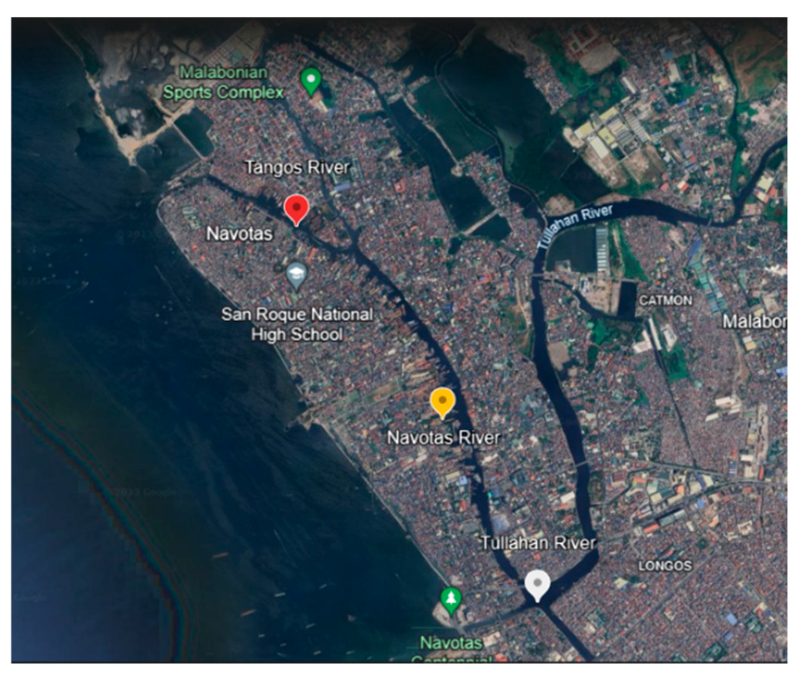
Figure 3.
The pH of Water in Navotas River during the Four-month Sampling Period.
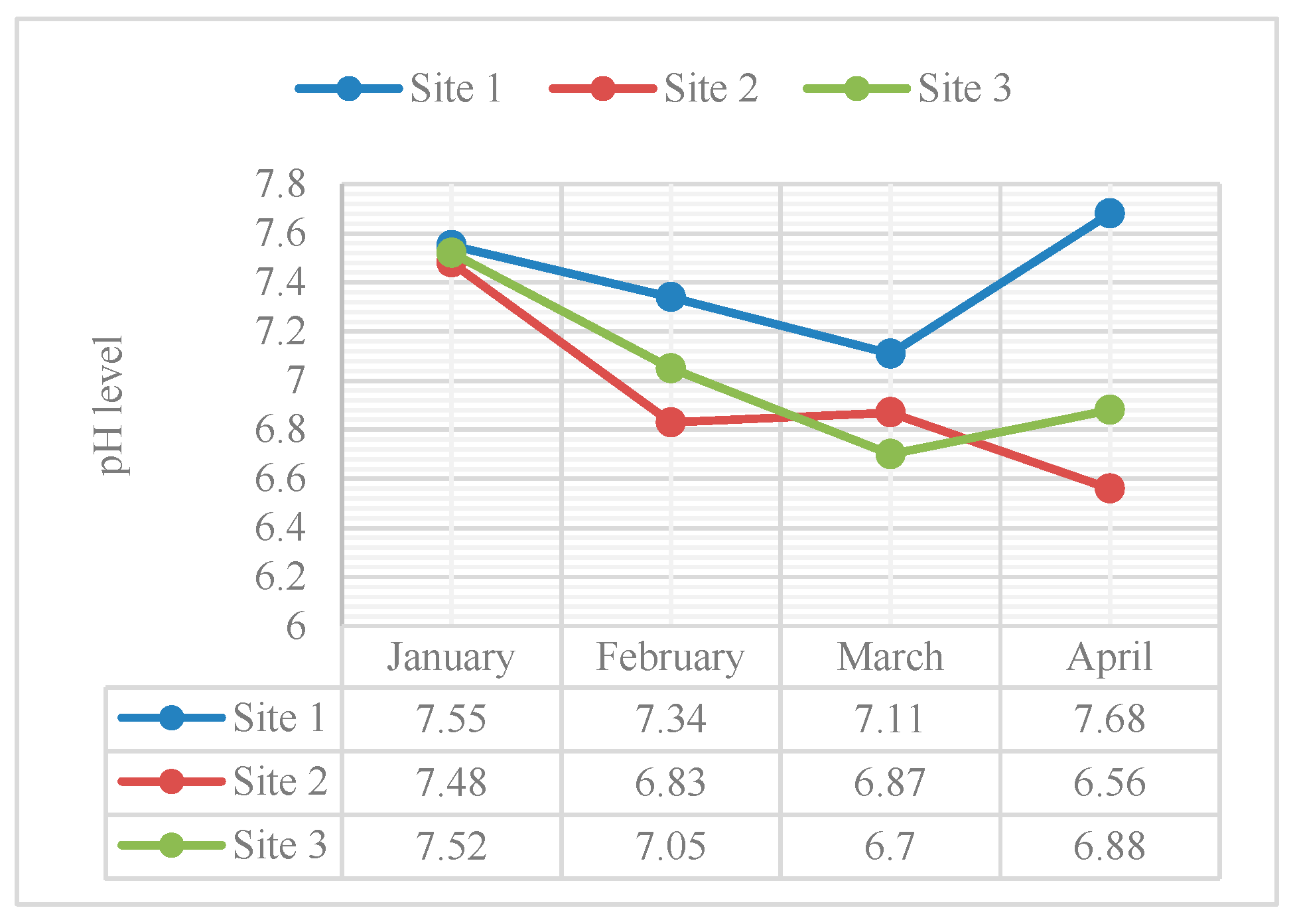
Figure 4.
The Temperature of Water in Navotas River during the Four-month Sampling Period.
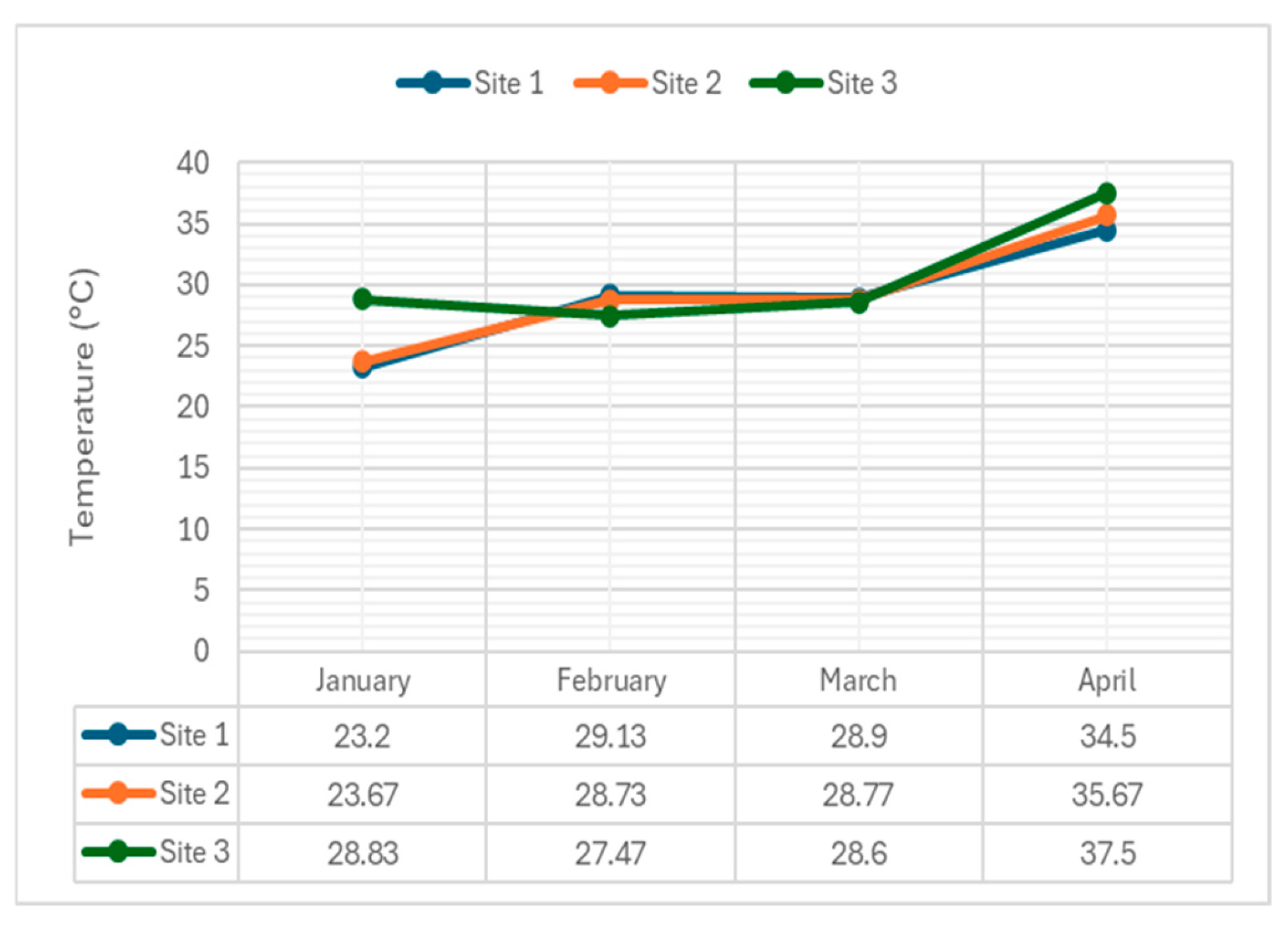
Figure 5.
The TDS of Water in Navotas River during the Four-month Sampling Period.
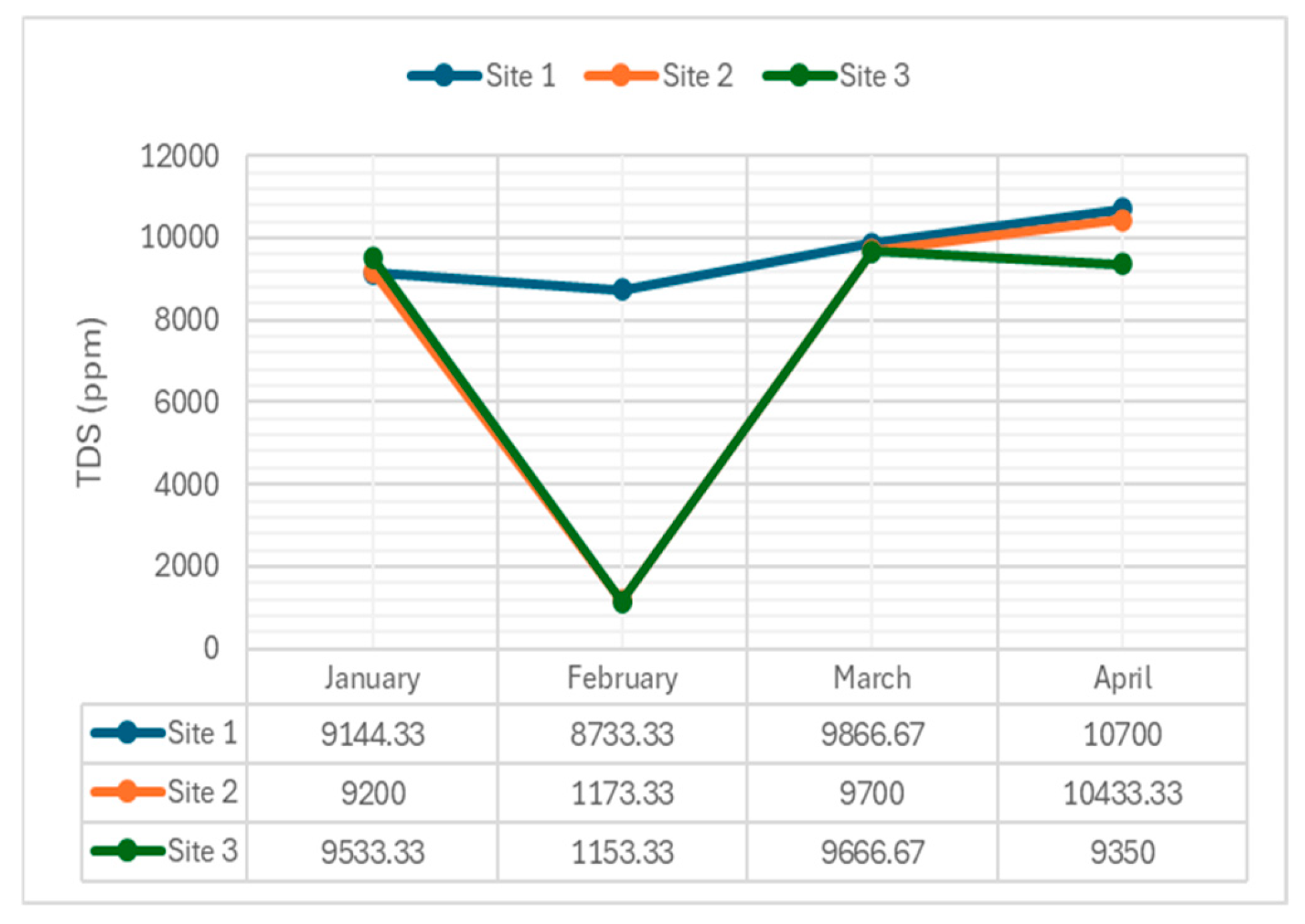
Figure 6.
The EC of Water in Navotas River during the Four-month Sampling Period.
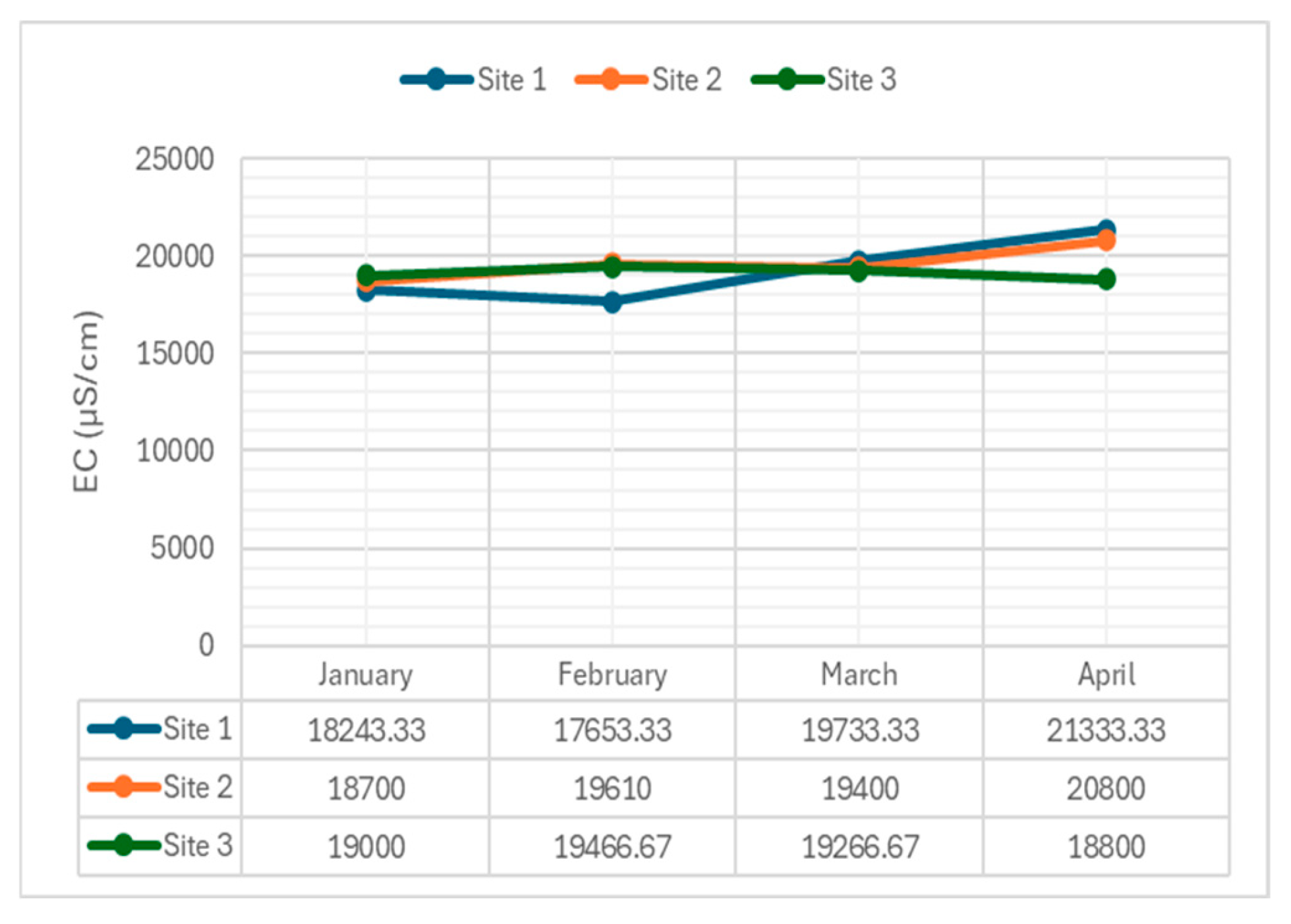
Figure 7.
The Secchi Disk Turbidity of Water in Navotas River during the Four-month Sampling Period.
Figure 7.
The Secchi Disk Turbidity of Water in Navotas River during the Four-month Sampling Period.
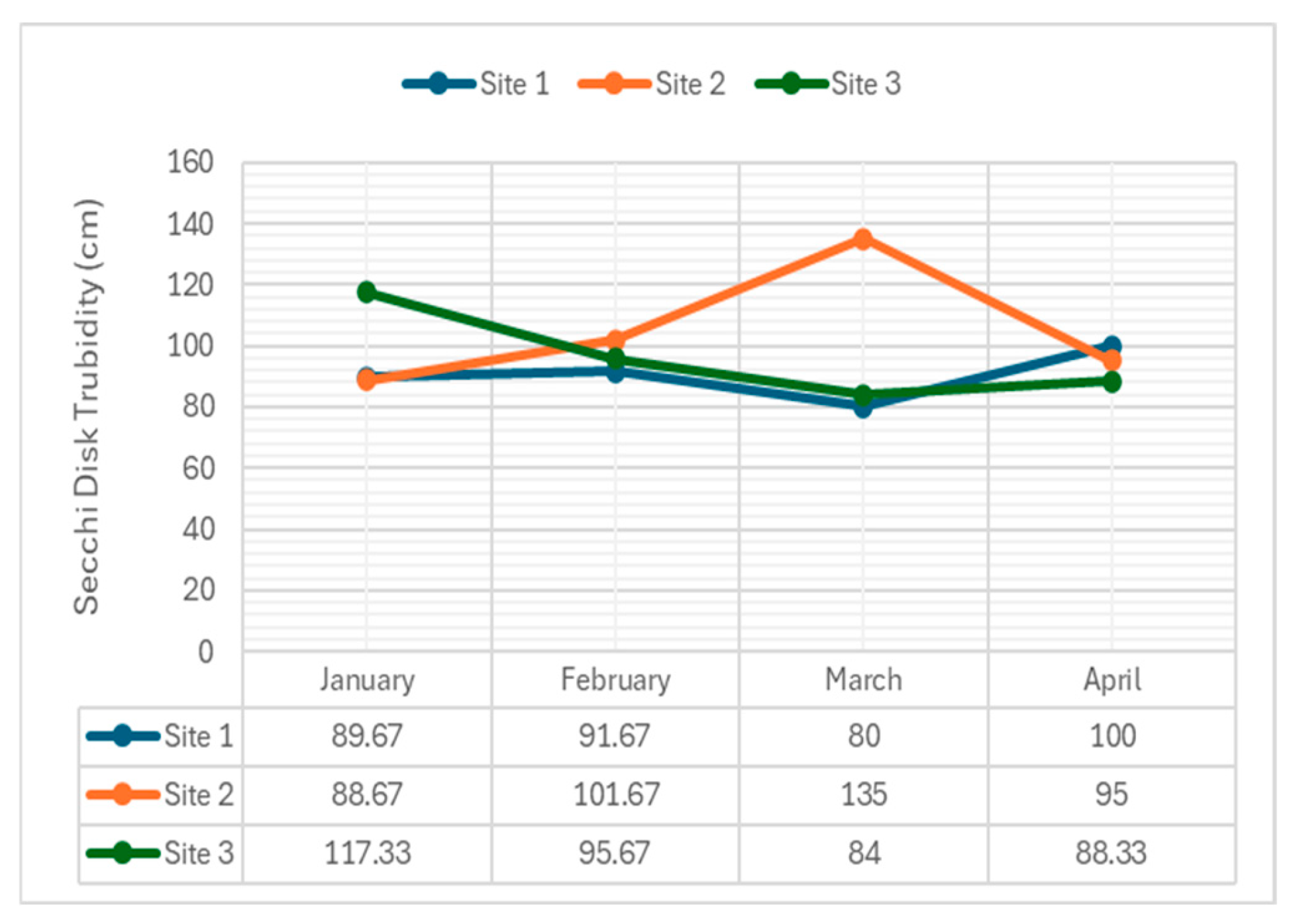
Figure 8.
The DO Level of Water in Navotas River during the Four-month Sampling Period.
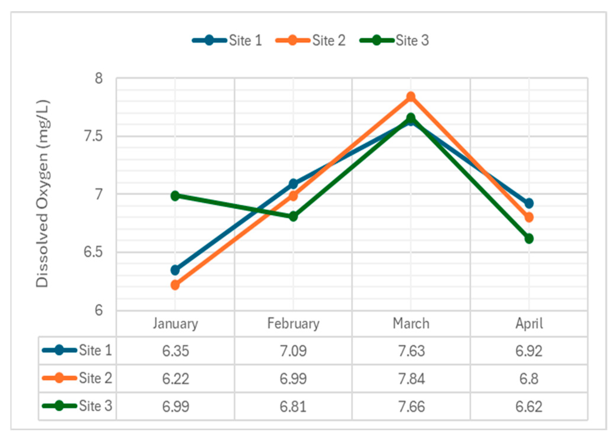
Figure 9.
The Nitrates (mg/L) of Water in Navotas River during the Four-month Sampling Period.
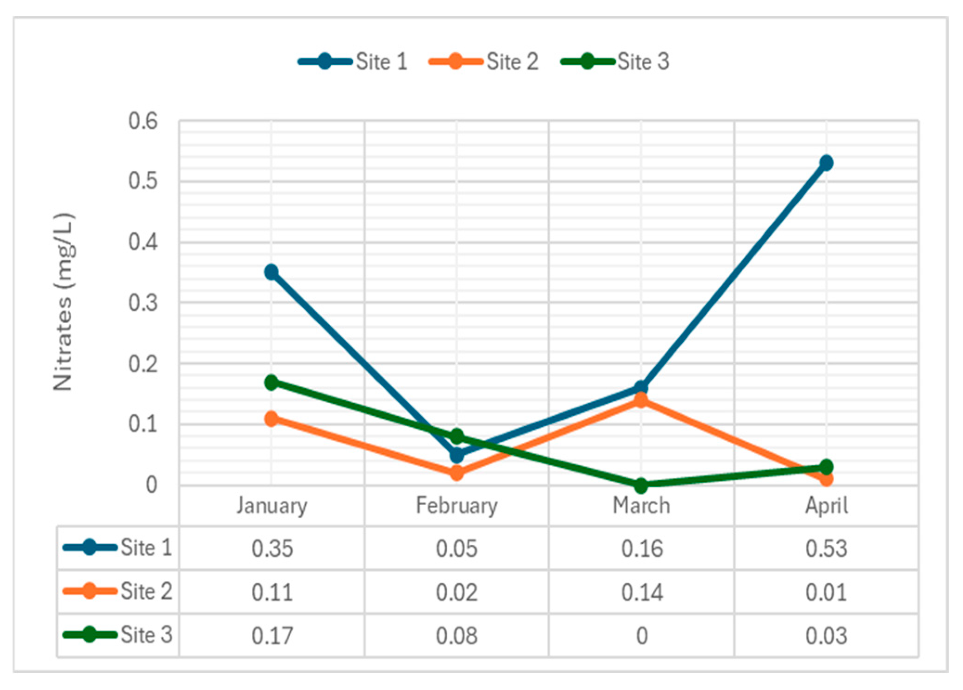
Figure 10.
The Phosphates (ppm) of Water in Navotas River during the Four-month Sampling Period.
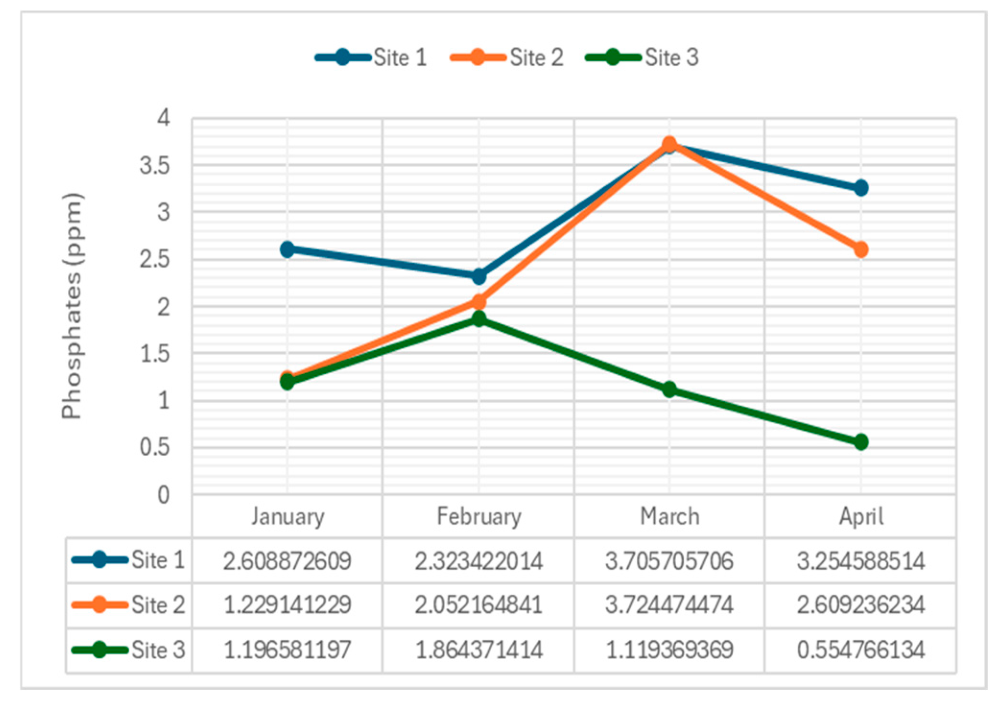
Figure 11.
The Fecal Coliform (MPN/100 mL) of Water in Navotas River during the Four-month Sampling Period.
Figure 11.
The Fecal Coliform (MPN/100 mL) of Water in Navotas River during the Four-month Sampling Period.

Table 1.
Anthropogenic Activities in Navotas River.
| Anthropogenic Activities | Mean | Remarks |
| Fishing | 2.86 | Often |
| Boating | 2.71 | Often |
| Washing of clothes | 2.29 | Seldom |
| Discharging water from the laundry | 2.29 | Seldom |
| Disposing of untreated wastewater from household and transport system | 2.00 | Seldom |
| Excreting domestic wastes | 1.14 | Never |
| Throwing garbage in the river | 1.07 | Never |
| Irrigating plants with water from the river | 1.00 | Never |
| Practicing aquaculture | 1.00 | Never |
Table 2.
Water Quality of Navotas Riverine Ecosystem during Four-month Sampling Period.
| Water Quality Parameter | Sampling Site |
Sampling Period | DENR Standard | |||
| Jan | Feb | Mar | Apr | |||
| pH | 1 | 7.55 | 7.3 | 7.1 | 7.68 | 6.5-9.0* |
| 2 | 7.48 | 6.83 | 6.87 | 6.56 | ||
| 3 | 7.52 | 7.05 | 6.70 | 6.88 |
||
| Temperature (°C) | 1 | 23.20 | 29.13 | 28.90 |
34.5 |
25-31* |
| 2 | 23.67 |
28.73 | 28.77 | 35.67 |
||
| 3 | 28.83 |
27.47 |
28.60 |
37.50 |
||
| TDS (mg/L) |
1 | 9144.33 |
8733.33 |
9866.67 |
10700 |
- |
| 2 | 9200 |
1173.33 |
9700 |
10433.33 |
||
| 3 | 9533.33 |
1153.33 |
9666.67 |
9350 | ||
| Conductivity (µS/cm) | 1 | 18243.33 |
17653.33 |
19733.33 |
21333.33 | - |
| 2 | 18700 |
19610 |
19400 |
20800 |
||
| 3 | 19000 |
19466.67 |
19266.67 |
18800 | ||
| Turbidity (NTU) |
1 | 5 |
5 |
6 |
5 |
- |
| 2 | 5 |
5 |
5 | 5 | ||
| 3 | 5 | 5 | 6 | 5 | ||
| Dissolved Oxygen (mg/L) | 1 | 6.35 | 7.09 | 7.63 | 6.92 | (minimum) 5* |
| 2 | 6.22 | 6.99 |
7.84 | 6.80 | ||
| 3 | 6.99 | 6.81 | 7.66 | 6.62 | ||
| Nitrates (mg/L) |
1 | 0.35 | 0.05 | 0.16 | 0.53 | 7* |
| 2 | 0.11 | 0.02 | 0.14 | 0.01 | ||
| 3 | 0.17 | 0.08 | <0.01 | 0.03 | ||
| Phosphates (mg/L) |
1 | 2.61 | 2.32 | 3.71 | 3.25 | 0.025** |
| 2 | 1.23 | 2.05 | 3.72 | 2.61 | ||
| 3 | 1.20 | 1.86 | 1.12 | 0.55 | ||
| Fecal Coliform (MPN/100mL) | 1 | 92000 | 160000 | 14000 | 350 | 200** |
| 2 | 35000 | 92000 | 160000 | 92000 | ||
| 3 | 160000 | 160000 | 92000 | 160000 | ||
Values enclosed in parentheses are the computed standard deviation of the measurements per site. *DAO 2016-08; **DAO 2021-19.
Table 3.
Kruskal-Wallis Test Results During the Sampling Periods.
| Parameters | January | February | March | April | ||||
| p-value | Remarks | p-value | Remarks | p-value | Remarks | p-value | Remarks | |
| pH | 0.925 | NS | 0.027 | S | 0.027 | S | 0.027 | S |
| Temperature | 0.058 | NS | 0.026 | S | 0.020 | S | 0.021 | S |
| TDS | 0.575 | NS | 0.065 | NS | 0.517 | NS | 0.027 | S |
| EC | 0.924 | NS | 0.190 | NS | 0.295 | NS | 0.035 | S |
| Turbidity | 0.066 | NS | 0.026 | S | 0.066 | NS | 0.148 | NS |
| DO | 0.027 | S | 0.027 | S | 0.295 | NS | 0.027 | S |
| Nitrates | 0.018 | S | 0.018 | S | 0.018 | S | 0.018 | S |
| Phosphates | 0.066 | NS | 0.050 | NS | 0.061 | NS | 0.027 | S |
| Fecal Coliform | 0.018 | S | 0.018 | S | 0.018 | S | 0.018 | S |
Table 4.
Friedman Test of the Sampling Sites.
| Parameters | Site 1 | Site 2 | Site 3 | |||
| p-value | Remarks | p-value | Remarks | p-value | Remarks | |
| pH | 0.029 | S | 0.042 | S | 0.029 | S |
| Temperature | 0.029 | S | 0.039 | S | 0.032 | S |
| TDS | 0.042 | S | 0.029 | S | 0.117 | NS |
| EC | 0.042 | S | 0.334 | NS | 0.958 | NS |
| Turbidity | 0.241 | NS | 0.051 | NS | 0.042 | S |
| Dissolved Oxygen | 0.029 | S | 0.029 | S | 0.029 | S |
| Nitrates | 0.029 | S | 0.029 | S | 0.029 | S |
| Phosphates | 0.029 | S | 0.029 | S | 0.042 | S |
| Fecal Coliform | 0.029 | S | 0.029 | S | 0.029 | S |
Table 5.
Water Quality Index of Navotas River during the Sampling Periods.
| WnQn | ||||||
| Parameter | January | February | March | April | ||
| pH | Site 1 | 3.48 | 3.38 | 3.27 | 3.54 | |
| Site 2 | 3.44 | 3.15 | 3.16 | 3.02 | ||
| Site 3 | 3.46 | 3.25 | 3.09 | 3.17 | ||
| Temperature | Site 1 | 30.88 | 38.77 | 38.46 | 45.92 | |
| Site 2 | 31.50 | 38.24 | 38.29 | 47.47 | ||
| Site 3 | 38.37 | 36.56 | 38.06 | 49.91 | ||
| Total Dissolved Solids | Site 1 | 1.22 | 1.16 | 1.31 | 1.42 | |
| Site 2 | 1.22 | 0.16 | 1.29 | 1.39 | ||
| Site 3 | 1.27 | 0.15 | 1.29 | 1.24 | ||
| Electrical Conductivity | Site 1 | 200.66 | 194.17 | 217.05 | 234.65 | |
| Site 2 | 205.68 | 215.69 | 213.38 | 228.78 | ||
| Site 3 | 208.98 | 214.12 | 211.92 | 206.78 | ||
| Turbidity | Site 1 | 6.65 | 6.65 | 7.99 | 6.65 | |
| Site 2 | 6.65 | 6.65 | 6.65 | 6.65 | ||
| Site 3 | 6.65 | 6.65 | 7.99 | 6.65 | ||
| Dissolved Oxygen | Site 1 | 5.87 | 6.55 | 7.05 | 6.40 | |
| Site 2 | 5.75 | 6.46 | 7.25 | 6.28 | ||
| Site 3 | 6.46 | 6.29 | 7.08 | 6.12 | ||
| Nitrates | Site 1 | 0.12 | 0.02 | 0.05 | 0.18 | |
| Site 2 | 0.04 | 0.01 | 0.05 | 0.00 | ||
| Site 3 | 0.06 | 0.03 | 0.00 | 0.01 | ||
| Phosphates | Site 1 | 347.36 | 308.77 | 493.76 | 432.54 | |
| Site 2 | 163.70 | 272.83 | 495.09 | 347.36 | ||
| Site 3 | 159.71 | 247.55 | 149.06 | 73.20 | ||
| Fecal Coliform | Site 1 | 3.06 | 5.32 | 3.06 | 0.01 | |
| Site 2 | 1.16 | 3.06 | 5.32 | 3.06 | ||
| Site 3 | 5.32 | 5.32 | 3.06 | 5.32 | ||
| Water Quality Index | 517 | 582 | 701 | 617 | ||
| Interpretation | Unfit | Unfit | Unfit | Unfit | ||
Table 6.
Distribution of Fish Species in Three Sites for the Four Sampling Periods.
| Family | Fish Species | Site 1 | Site 2 | Site 3 | Total Occurrence (%) |
| Scatophagidae | Scatophagus argus (kitang) | 31 | 8 | 11 | 50 (18.59%) |
| Terapontidae | Pelates quadrilineatus (babanse) | 26 | 8 | 15 | 49 (18.22%) |
| Cichlidae | Sarotherodon melanotheron (gloria tilapia) | 26 | 7 | 13 | 46 (17.10%) |
| Terapontidae | Terapon jarbua (bagaong) | 27 | 9 | 6 | 42 (15.61%) |
| Lutjanidae | Lutjanus argentimaculatus (alakaak) | 17 | 3 | 14 | 34 (12.64%) |
| Lutjanidae | Lutjanus argentimaculatus (kabang) | 21 | 3 | 2 | 26 (9.67%) |
| Dorosomatidae | Nematalosa nasus (kabase) | 13 | 8 | 1 | 22 (8.18%) |
| Total | 161 | 46 | 62 | 269 (100%) |
Table 7.
Species Importance Value of the Ichthyofaunal Species in Navotas River.
| Species | RF | RD | RA | SIV | Rank |
| Scatophagus argus (kitang) | 16.67 | 18.59 | 18.58 | 53.84 | 1 |
| Pelates quadrilineatus (babanse) | 14.58 | 18.21 | 18.23 | 51.02 | 2 |
| Sarotherodon melanotheron (gloria tilapia) | 16.67 | 17.10 | 17.10 | 50.87 | 3 |
| Terapon jarbua (bagaong) | 14.58 | 15.61 | 15.62 | 45.81 | 4 |
| Lutjanus argentimaculatus (alakaak) | 12.50 | 12.64 | 12.65 | 37.79 | 5 |
| Lutjanus argentimaculatus (kabang) | 14.58 | 9.67 | 9.66 | 33.91 | 6 |
| Nematalosa nasus (kabase) | 10.42 | 8.18 | 8.17 | 26.76 | 7 |
Table 8.
Biodiversity Status of Collected Fish Species in Navotas River.
| Family | Species | Common Name | Biodiversity Status | Conservation Status |
| Scatophagidae | Scatophagus argus | Kitang | Native | Least Concern |
| Dorosomatidae | Nematalosa nasus | Kabase | Native | Least Concern |
| Terapontidae | Terapon jarbua | Bagaong | Native | Least Concern |
| Pelates quadrilineatus | Babanse | Native | Not Evaluated | |
| Lutjanidae | Lutjanus argentimaculatus | Alakaak | Native | Least Concern |
| Lutjanus argentimaculatus | Kabang | Native | Least Concern | |
| Cichlidae | Sarotherodon melanotheron | Gloria Tilapia | Introduced | Least Concern |
Table 9.
Species Diversity of Ichthyofauna in Navotas River.
| Diversity Index | Sampling Sites | ||
| Site 1 | Site 2 | Site 3 | |
| Shannon-Wiener (H’) | 1.91 | 1.87 | 1.71 |
| Simpson’s Diversity (D) | 0.15 | 0.14 | 0.18 |
| Simpson’s Index of Diversity (1-D) | 0.85 | 0.86 | 0.82 |
| Reciprocal (1/D) | 6.81 | 7.04 | 5.48 |
| Margalef’s Richness (dmg) | 1.18 | 1.57 | 1.45 |
Table 10.
Sorensen’s Coefficient Similarity Index for Sampling Sites.
| Sites | % Similarity |
| Site1-Site2 | 60% |
| Site1-Site3 | 80% |
| Site2-Site3 | 60% |
Table 1.
Table type styles (Table caption is indispensable).
| Table Head | Table Column Head | ||
| Table column subhead | Subhead | Subhead | |
| copy | More table copya | ||
a. Sample of a Table footnote (Table footnote is dispensable).
Disclaimer/Publisher’s Note: The statements, opinions and data contained in all publications are solely those of the individual author(s) and contributor(s) and not of MDPI and/or the editor(s). MDPI and/or the editor(s) disclaim responsibility for any injury to people or property resulting from any ideas, methods, instructions or products referred to in the content. |
© 2024 by the authors. Licensee MDPI, Basel, Switzerland. This article is an open access article distributed under the terms and conditions of the Creative Commons Attribution (CC BY) license (http://creativecommons.org/licenses/by/4.0/).
Copyright: This open access article is published under a Creative Commons CC BY 4.0 license, which permit the free download, distribution, and reuse, provided that the author and preprint are cited in any reuse.


