1. Introduction
Solving partial differential equations (PDEs) is of paramount interest in numerous fields of science and engineering, as they form the foundation for modeling a wide range of physical phenomena. PDEs describe the behavior of physical systems over space and time, governing processes such as heat transfer [
1], fluid dynamics [
2], structural mechanics [
3], and electromagnetics [
4]. Accurate and efficient solutions to PDEs are crucial for advancing research and development in these areas, making them a focal point of computational and analytical studies [
5]. Traditional methods for solving PDEs, such as finite element (FEM), finite difference, and finite volume methods, can be computationally intensive, especially for high-dimensional problems and complex geometries. In recent years, Physics-Informed Neural Networks (PINNs) have emerged as a powerful alternative computational framework that integrates machine learning with fundamental physical laws to address these challenges [
6,
7].
By embedding physical constraints directly into the neural network’s loss function
cf. Eq. (
1), they utilize both data loss
, cf. Eq. (2) and physics loss
, cf. Eq. (3) components. With
as the weighting factor for the data component of the total loss.
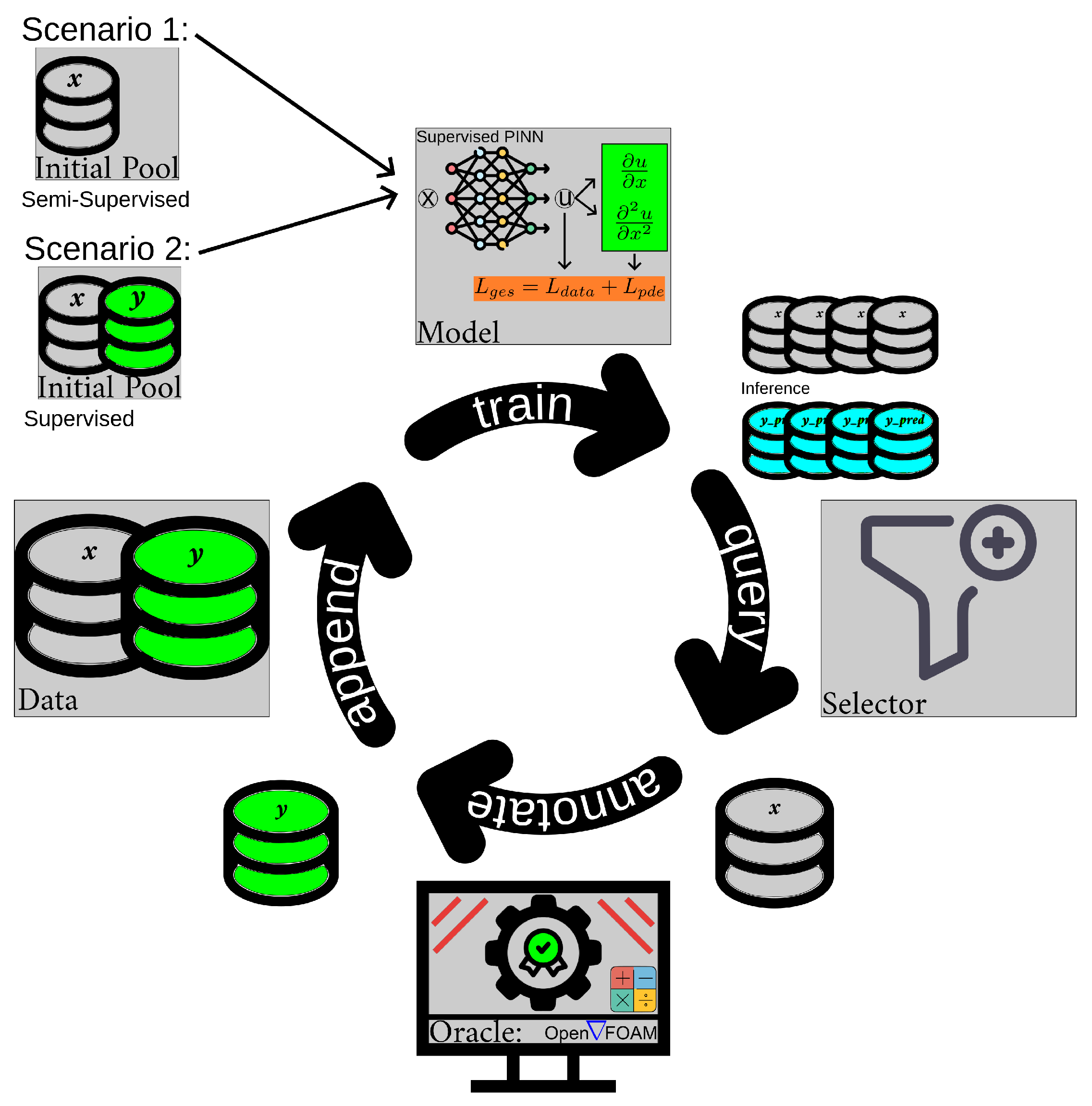
PINNs offer several advantages over traditional methods and ensure that the solutions are not only data-consistent but also physically accurate. In
Figure 1 an active learning (AL) cycle with a PINN as
Model is depicted. The queries from the
Selector are directed towards an
Oracle which is in our case a FEM simulation. The AL cycle uses Eq. (
1) where
measures the mean squared error between a predicted
u and a true
solution variable (for instance, the prediction of the electric potential), and is therefore trained in a supervised manner.
While the physics loss Eq. (3)
uses the residual
and ensures adherence to the PDE. This loss term operates solely unsupervised on the predicted solution variable
u. This integration allows PINNs to handle sparse data effectively, making them particularly useful in real-world applications where data is limited [
6].
We use this AL cycle to train the PINN starting from two different initial states. In Scenario 1 the model is initially trained completely unsupervised, using the physics-informed loss (3) only, and then data is provided by the oracle to continue the following iterations semi-supervised on . In Scenario 2, we use ground-truth data for supervised training right from the start and therefore use as a loss function. Additionally, to these two modes of training, PINNs can naturally incorporate multi-physics problems and seamlessly handle high-dimensional spaces, providing a flexible and efficient approach to solving complex PDEs.
The choice of mesh plays a crucial role in the implementation of PINNs, as it defines the discretization of the problem domain. Structured meshes, with their equidistantly distributed cells, offer computational efficiency and simplicity by enabling straightforward application of automatic differentiation algorithm to compute spatial gradients [
8]. In contrast, unstructured meshes provide the flexibility to handle complex geometries and allow for adaptivity in regions requiring higher resolution. Graph Neural Networks (GNNs) are ideal for solving PDEs on unstructured meshes because they adeptly handle the complex, irregular topologies of these meshes by learning node relationships directly. However, the computation of spatial gradients in unstructured meshes is more complex due to the irregular neighborhoods of their triangular cells. The design of the mesh significantly affects the distribution of data points, the precision of differential operator evaluations, and the enforcement of boundary conditions. For this reason, we integrate the concepts of PINNs and GNNs to develop a Physics-Informed Graph Neural Network PIGNN. For that, we have to adapt an existing TensorFlow library to enable the computation of field gradients on unstructured meshes in our PyTorch model.
In summary, PINNs represent a sophisticated method for solving PDEs by integrating neural networks with physical laws. Enhancing these networks through AL by physical loss residuals, rather than explicit uncertainty quantification, allows for a more straightforward yet effective refinement process. Strategic mesh design further augments the model, making PIGNNs a versatile tool for a wide range of applications in science and engineering.
The remainder of this article is structured as follows: in
Section 2 we summarize the related work before we introduce our methodology in
Section 3. Our preliminary results are presented in
Section 4. The article concludes with a summary of our findings and an outlook for future work in
Section 5.
2. Related Work
In this section, we propose related work to the topics of GNNs and PINNs as well as AL and PINNs.
GNNs and PINNs:
Solving mesh-based PDEs with neural networks is an increasingly progressive topic of research. Typical data-driven solution methods come from the fields of computer vision and graph-based learning [
2]. However, these methods lack information about the underlying physics of the problems at hand.
Initial studies have demonstrated that combining GNNs and PINNs yields excellent results in various scientific and engineering applications. GNNs excel at processing data represented as graphs, which is particularly useful for handling complex relationships in unstructured meshes [
9,
10]. To leverage GNNs on unstructured meshes for our research, it is essential to modify an existing package [
11], initially developed for TensorFlow, to facilitate its integration with PyTorch. This adaptation ensures that the capabilities of GNNs can be effectively utilized to design PINNs with the ability to solve equations containing field gradients.
AL and PINNs:
AL for regression tasks is highly effective in reducing the computational load associated with simulating PDEs. By strategically selecting the most informative samples for extensive simulation, AL can significantly enhance efficiency [
12,
13]. However, for specific applications like design optimization, where the goal is to systematically identify the optimal design parameters that satisfy specified performance criteria, it is essential to customize the query strategies. This customization ensures that iterative algorithms effectively find the best design with minimal PDE evaluations, aligning the AL process with the optimization objectives and constraints of the physical system described by PDEs [
14].
The idea of combining PINNs with AL is gaining increasing attention. Recent works have taken initial steps in this direction, employing uncertainty sampling via Monte Carlo dropout [
15] to select informative samples. Another study proposed an adaptive sampling strategy based on Christoffel functions [
16]. In contrast to these approaches, our work focuses exclusively on a score-sampling strategy based on the physical loss.
3. Methodology
Our methodology is structured as follows: initially, we introduce the data, which is derived from the Poisson equation. Subsequently, we present our model, query strategy, and oracle. Finally, we present our experimental setup.
Data:
As dataset we use the charge density input array and the FEM simulated solutions of the Poisson equation together with the mesh, featuring a circular bounded domain (
), and the associated edge indices. As input scalar field
f we use a random distribution of circular areas with randomly chosen radii. Although the Poisson equation can be applied to a variety of physics problems, our goal is to calculate the electric potential field
u of a given constant charge density distribution
f, represented by the circle areas which is expressed in Eq. (
4). Here
represents the Laplacian operator:
In this equation,
denotes the boundary of the domain
. In
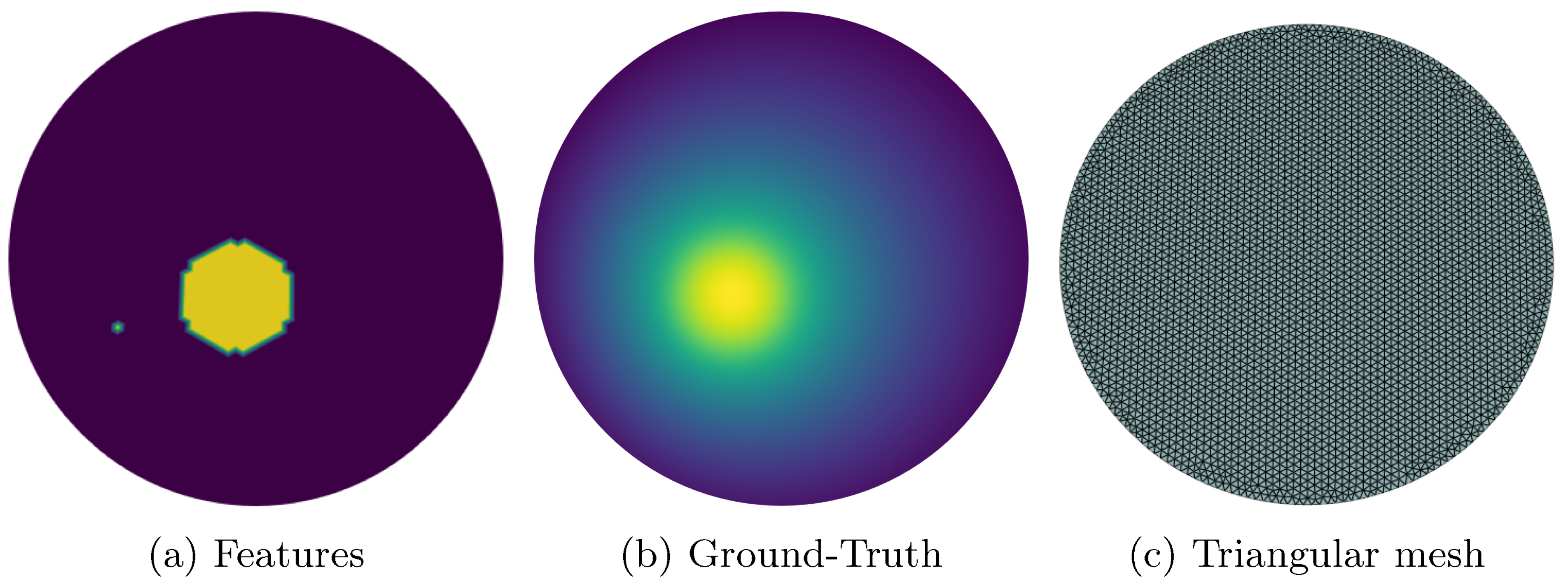
Figure 2, the input features (
Figure 2a) and the ground-truth solution (
Figure 2b) of a random sample are exemplarily illustrated.
As illustrated in Figure , we employ an unstructured triangular mesh to discretize the domain. This type of mesh allows us to accurately capture the geometry and boundary conditions of complex domains. The physical loss
of the Poisson equation (Eq. (
4)) is defined in Eq. (
5):
To compute this loss, it is necessary to obtain the second spatial derivative, indicated by the Laplace operator. This computation requires considering the spatial dependencies of the mesh cells. While the Automatic Differentiation (AD) algorithm [
8,
17] is typically used for uniform and structured meshes, it cannot be applied to unstructured meshes used in our study because it struggles with efficiently propagating derivatives through the complex and irregular connections. Therefore, specialized techniques are needed to handle the unstructured nature of the mesh and accurately compute the required gradients for the physical loss.
Model:
We utilize our PIGNN to efficiently handle the intricate geometries of the domain. The GNN’s structure is particularly well-suited for capturing the relationships and dependencies within unstructured data. As GNN type we chose six chebyshev spectral graph convolutional (ChebConv) layers as the main model and two feed-forward layers as encoder and decoder. The ChebConv layers
k-hop convolutional operator aggregates information of vertices that are in a radius of
k-hops from the central vertex in contrast to the more popular 1-hop graph convolutional layers, which only take into account directly connected nodes. Using a
k-factor of six allows our model to recognize bigger structures and helps to minimize the prediction error. To enhance the model’s capability in dealing with complex mesh geometries, we integrate it with the MeshGradientPy package [
11], which computes field gradient estimates on every cell based on linear interpolation and then uses an averaging method to obtain gradient values on vertices. This integration is crucial for accurately resolving the Laplacian, as specified in Eq. (
5). By doing so, we can effectively calculate the unsupervised physical loss
, ensuring that the model adheres to the underlying physical laws governing the problem domain. Since the package is developed for Tensorflow, we adapted the implementation for integration with PyTorch.
Query Strategy:
During inference, we can compute the physics residuals without needing ground-truth values. These residuals are derived from the physical loss , highlighting samples of the PIGNN’s predictions that deviate from expected physical behavior. To improve the performance of our PIGNNs, we employ an innovative strategy that leverages the physical loss during inference to guide AL and retraining.
In Eq. (
6) our query strategy is depicted. Let
S be the set of all samples
x that are inferred, and
T be a subset of
S containing the
n samples with the highest
values. The subset
T is forwarded to the
Oracle for target value acquisition.
This strategy works by evaluating the physical residuals, which quantify how well the predicted solution variable
u adheres to the governing physical laws. By identifying samples where the model’s predictions are less reliable, we can target specific areas for model improvement. The advantage of this approach is that we can quantify the physical loss in an unsupervised manner, thereby eliminating the need for costly epistemic uncertainty quantification methods [
18].
This unsupervised quantification of physical loss simplifies the AL process, allowing the model to autonomously identify and focus on regions with high residuals. These high-residual areas indicate where the model’s predictions are most inaccurate, guiding the addition of new data points or retraining efforts to these critical areas. This method not only streamlines the training process but also ensures robust model enhancement by continuously refining the model based on its internal assessments of physical law adherence. This approach is particularly valuable in scenarios where obtaining ground-truth data is expensive or impractical, as it maximizes the use of available information to improve model performance and reliability.
Oracle:
Focusing on samples with high physical residuals, the Oracle generates additional data in these regions, thereby improving the model’s performance. The Model uses its internal physics-based evaluations to guide its learning process, leveraging both the supervised and unsupervised capabilities of the PIGNN to ensure its predictions remain physically consistent. The Selector identifies high-residual samples and the Oracle provides the corresponding true values, which the Model then uses to refine its predictions. This active interaction between the Oracle and the Model allows for targeted improvements in areas where the model’s predictions are less reliable enhancing the model’s performance in a cost-effective way.
By comparing these two scenarios, we aim to determine the effectiveness of incorporating high-fidelity data versus relying mostly on the model’s unsupervised physical insights.
Experimental Setup:
Our experimental setup is designed to evaluate two distinct scenarios and is depicted in
Figure 1:
In
Scenario 1, we start with a pool of 1500 samples with ground-truth solution data determined from FEM simulations (oracle). The PIGNN is initially trained on 600 randomly selected samples in an unsupervised manner using the physics-based loss function
(cf. Eq. (3)) only, therefore, no ground-truth data is provided. After this initial training phase, the model is evaluated on the remaining 900 samples, calculating physics residuals to identify the 60 samples with the highest residuals (cf. Eq.(
6)). The ground-truth values for these high-residual samples are then obtained from the
Oracle and added to the training set, enabling the use of the total loss Eq. (
1) on these additionally acquired samples. This iterative process of identifying and adding 60 high-residual samples continues until the cycle iterates 5 times. This scenario is termed semi-supervised since the majority of the training is based on the unsupervised physical loss (cf. Eq. (3)) only, except for the samples added by the oracle.
In
Scenario 2, we defined a supervised scenario, therefore, using the ground-truth data of the initial 600 randomly selected samples. The total loss
(cf. Eq. (
1)) is applied to both, the initial samples and the samples acquired over five iterations, which are provided by the oracle.
For both scenarios, after each iteration, the PIGNN is tested on a separate test dataset of 1500 samples to evaluate its prediction performance and adherence to physical laws. Additionally, we compare these methods to a random selection strategy, where 60 random samples are acquired for the training set in each iteration. This comparison assesses the efficiency of the proposed selection strategy guided by the physical loss .
4. Preliminary Results and Discussion
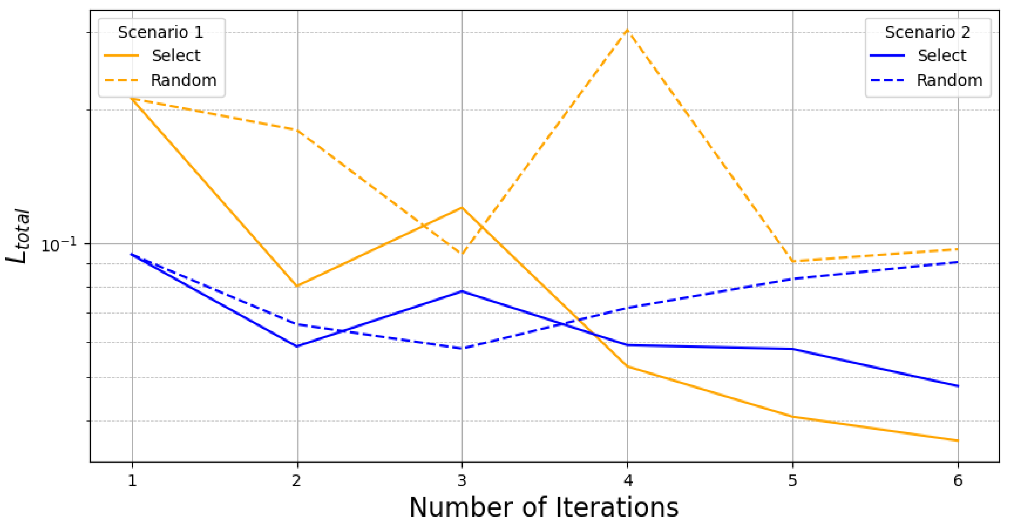
The results of our experiments, are summarized in
Figure 3 and will be discussed in the following:
First, we can observe that our proposed query strategy outperforms the random strategy in both scenarios. It is evident that after the first iteration, Scenario 2, which was trained supervised to optimize the total loss , surpasses Scenario 1, where the model was trained solely using the unsupervised loss . However, after four AL cycles, Scenario 1 demonstrates superior performance compared to Scenario 2. This indicates that the initial unsupervised training is a viable approach for our PIGNN. Considering that substantial resources are saved by determining the ground-truth values for the initial training pool — which in our example involved 600 samples — and given that one FEM simulation in industrial use cases can take days or even weeks of computing time, the advantages become even more apparent. An adaptive approach that only simulates the most valuable samples presents significant benefits.
However, an in-depth analysis of the consistency of multiple runs using various seeds was beyond the scope of this work. Additionally, we did not conduct any hyper-parameter tuning or investigate AL parameters such as the initial pool size, the acquisition size, or the total budget. Other typical AL query strategies were also not considered. Another critical parameter is
, which serves as the weighting factor between the two components of the loss function (cf. Eq. (
1)). An incorrectly chosen
can lead to the optimization being dominated by one part of the loss function, either
or
, at the expense of the other. These aspects need to be elaborated in future work.
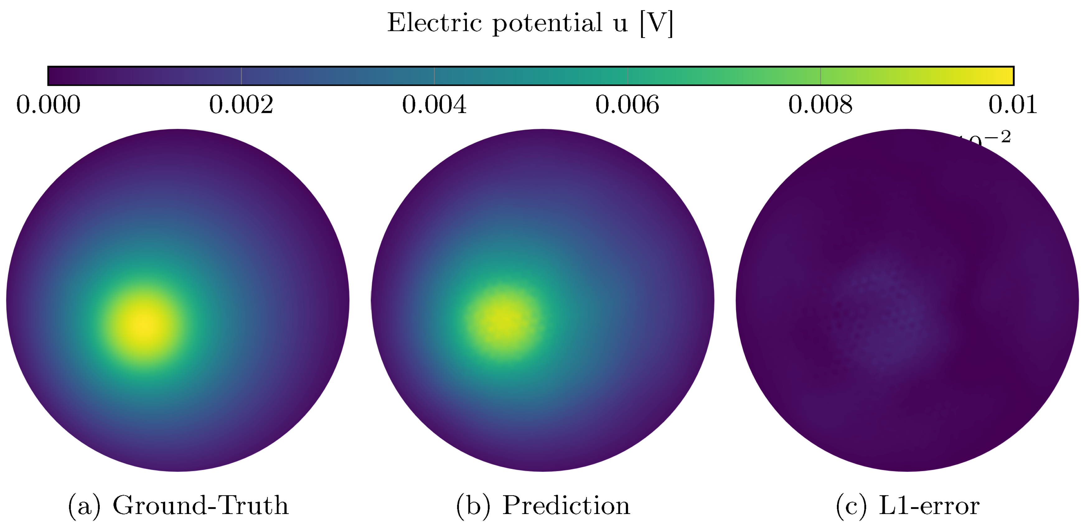
In
Figure 4 a randomly chosen test sample of the final iteration of
Scenario 1 is depicted. It shows that our AL strategy in combination with the PIGNN is capable of providing high-performing predictions in
Figure 4b. In
Figure 4c the absolute deviation e.g. the L1-error between the prediction and the ground-truth solution is depicted.
5. Conclusion, Limitations and Future Work
Our experiments show that our PIGNN is generally suitable for use in AL scenarios. Our proposed query strategy is built upon the network’s physical loss, which can be evaluated unsupervised. In future work, we aim to apply our methodology and model to real-world problems and more complex datasets from the field of fluid dynamics [
19] and electrodynamics [
4]. Further, we plan to investigate other acquisition sizes, total budgets, and the initial selection of samples as well as optimization of hyper-parameters which is in general not trivial in deep AL [
20].
Currently, our PIGNN is validated on a circular problem domain solving the Poisson equation on an unstructured triangular mesh. In the future, we plan to employ this model for more complex geometries and physical problems. For the above-mentioned datasets, we intend to solve the Maxwell equations on an unstructured mesh for modeling an electric motor and address turbulent flow in a U-bend applying the Navier-Stokes equations on a graded mesh. Another work compares methods from the fields of computer vision and graph learning on these two datasets [
2]. We aim to extend this comparison to include PINNs. These advancements will help validate the robustness and versatility of our PIGNN in solving a wider range of complex real-world problems. Furthermore, we want to contribute with the help of AL to face the problems of data scarcity in the realm of solving computationally expensive PDEs.
References
- S. Cai, Z. Wang, S. Wang, P. Perdikaris, and G. E. Karniadakis, “Physics-Informed Neural Networks for Heat Transfer Problems,” Journal of Heat Transfer, vol. 143, p. 060801, 04 2021.
- J. Decke, O. Wünsch, B. Sick, and C. Gruhl, “From structured to unstructured: A comparative analysis of computer vision and graph models in solving mesh-based pdes,” 2024.
- E. Haghighat, M. Raissi, A. Moure, H. Gomez, and R. Juanes, “A physics-informed deep learning framework for inversion and surrogate modeling in solid mechanics,” Computer Methods in Applied Mechanics and Engineering, vol. 379, p. 113741, 2021.
- D. Botache, J. Decke, W. Ripken, et al., “Enhancing multi-objective optimization through machine learning-supported multiphysics simulation,” 2023.
- S. H. Rudy, S. L. Brunton, J. L. Proctor, and J. N. Kutz, “Data-driven discovery of partial differential equations,” Science Advances, vol. 3, no. 4, p. e1602614, 2017.
- M. Raissi, P. Perdikaris, and G. Karniadakis, “Physics-informed neural networks: A deep learning framework for solving forward and inverse problems involving nonlinear partial differential equations,” Journal of Computational Physics, vol. 378, pp. 686–707, 2019.
- S. Cuomo, V. S. di Cola, F. Giampaolo, G. Rozza, M. Raissi, and F. Piccialli, “Scientific machine learning through physics-informed neural networks: Where we are and what’s next,” 2022.
- A. G. Baydin, B. A. Pearlmutter, A. A. Radul, and J. M. Siskind, “Automatic differentiation in machine learning: a survey,” J. Mach. Learn. Res., vol. 18, p. 5595–5637, jan 2017.
- H. Gao, M. J. Zahr, and J.-X. Wang, “Physics-informed graph neural galerkin networks: A unified framework for solving pde-governed forward and inverse problems,” Computer Methods in Applied Mechanics and Engineering, vol. 390, p. 114502, Feb. 2022.
- A. Thangamuthu, G. Kumar, S. Bishnoi, R. Bhattoo, N. M. A. Krishnan, and S. Ranu, “Unravelling the performance of physics-informed graph neural networks for dynamical systems,” in Advances in Neural Information Processing Systems, vol. 35, pp. 3691–3702, Curran Associates, Inc., 2022.
- C. Mancinelli, M. Livesu, and E. Puppo, “A comparison of methods for gradient field estimation on simplicial meshes,” Computers & Graphics, vol. 80, pp. 37–50, 2019.
- P. Kumar and A. Gupta, “Active learning query strategies for classification, regression, and clustering: A survey,” J. Comput. Sci. Technol., vol. 35, no. 4, p. 913–945, 2020.
- L. Rauch, M. Aßenmacher, D. Huseljic, M. Wirth, B. Bischl, and B. Sick, “Activeglae: A benchmark for deep active learning with transformers,” in Machine Learning and Knowledge Discovery in Databases: Research Track, p. 55–74, Springer Nature Switzerland, 2023.
- J. Decke, C. Gruhl, L. Rauch, and B. Sick, “DADO -- Low-cost query strategies for deep active design optimization,” in 2023 International Conference on Machine Learning and Applications (ICMLA), pp. 1611–1618, IEEE, 2023.
- Y. Aikawa, N. Ueda, and T. Tanaka, “Improving the efficiency of training physics-informed neural networks using active learning,” New Generation Computing, pp. 1–22, 2024.
- J. M. Cardenas, B. Adcock, and N. Dexter, “Cs4ml: A general framework for active learning with arbitrary data based on christoffel functions,” Advances in Neural Information Processing Systems, vol. 36, 2024.
- B. van Merrienboer, O. Breuleux, A. Bergeron, and P. Lamblin, “Automatic differentiation in ml: Where we are and where we should be going,” in Advances in Neural Information Processing Systems, vol. 31, 2018.
- D. Huseljic, B. Sick, M. Herde, and D. Kottke, “Separation of aleatoric and epistemic uncertainty in deterministic deep neural networks,” in 2020 25th International Conference on Pattern Recognition (ICPR), pp. 9172–9179, 2021.
- J. Decke, O. Wünsch, and B. Sick, “Dataset of a parameterized U-bend flow for deep learning applications,” Data in Brief, vol. 50, p. 109477, 2023.
- D. Huseljic, M. Herde, P. Hahn, and B. Sick, “Role of hyperparameters in deep active learning,” in Workshop on Interactive Adaptive Learning (IAL), ECML PKDD, pp. 19–24, 2023.
|
Disclaimer/Publisher’s Note: The statements, opinions and data contained in all publications are solely those of the individual author(s) and contributor(s) and not of MDPI and/or the editor(s). MDPI and/or the editor(s) disclaim responsibility for any injury to people or property resulting from any ideas, methods, instructions or products referred to in the content. |
© 2024 by the authors. Licensee MDPI, Basel, Switzerland. This article is an open access article distributed under the terms and conditions of the Creative Commons Attribution (CC BY) license (http://creativecommons.org/licenses/by/4.0/).


