Submitted:
11 July 2024
Posted:
12 July 2024
You are already at the latest version
Abstract
Keywords:
1. Introduction
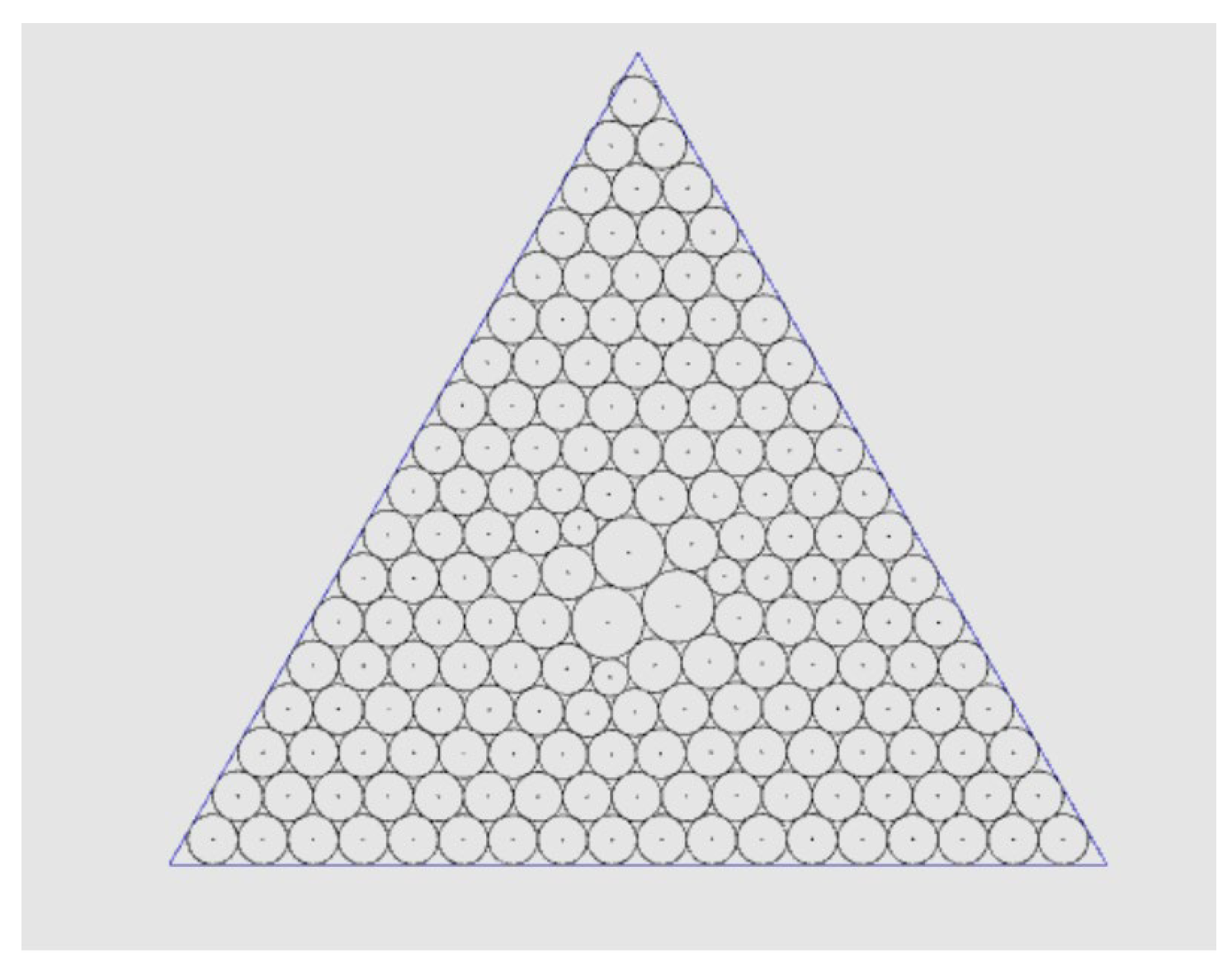
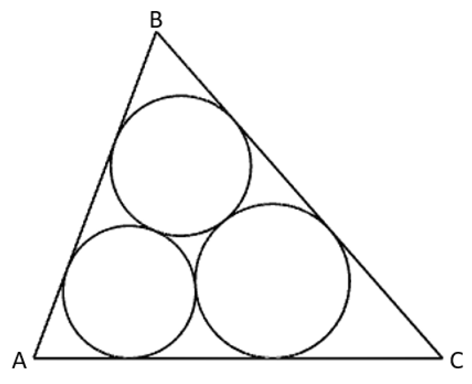
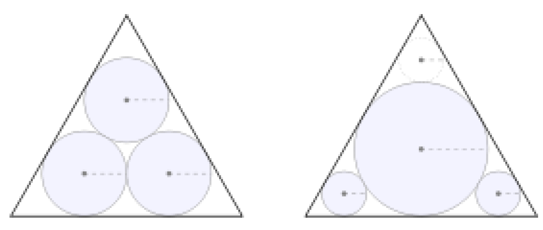
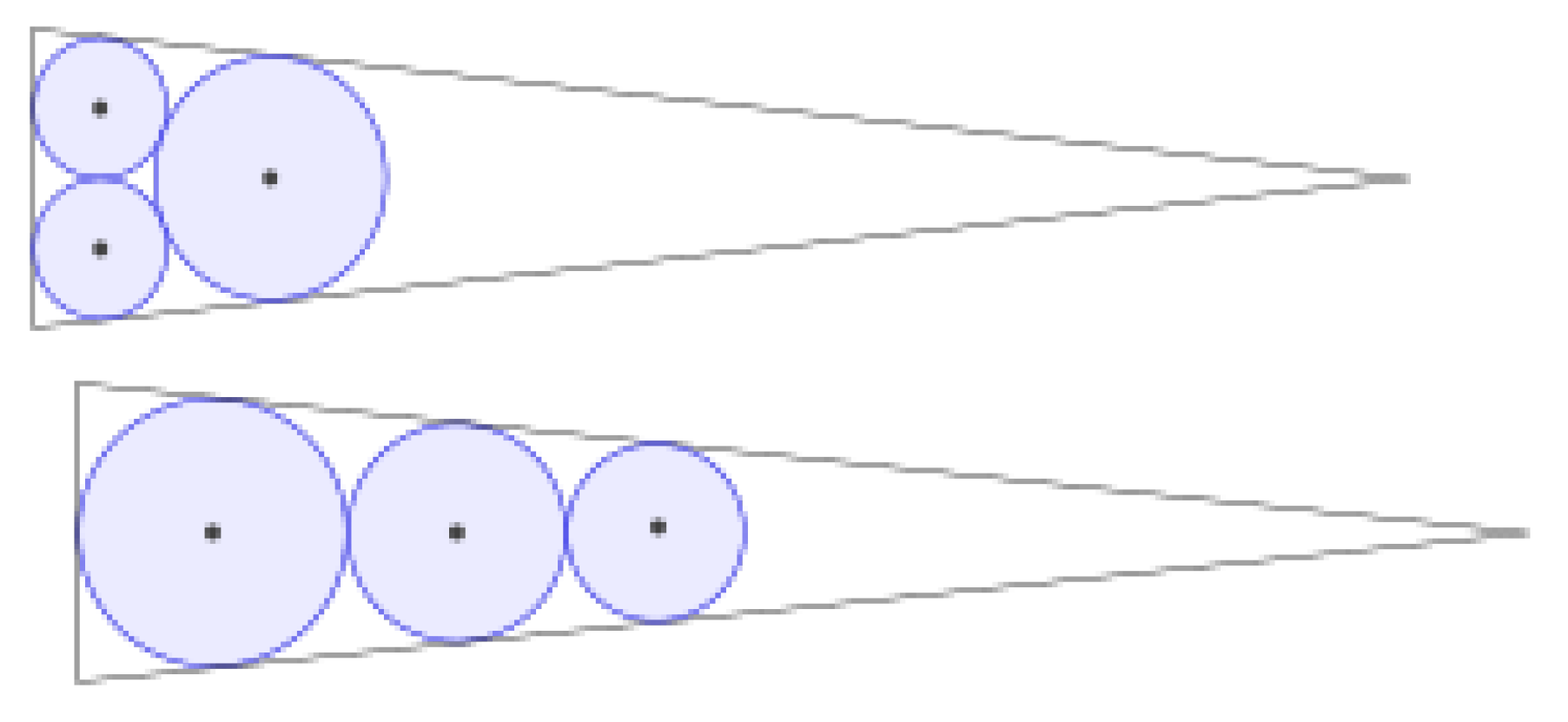
1.1. Malfatti’s Problem and Extended General Malfatti’s Problem
- Input the coordinate of 3 vertices A, B, C; Calculate the angle A, B, C, and the edge length c.
- Set a tolerance variable eps = 0.01
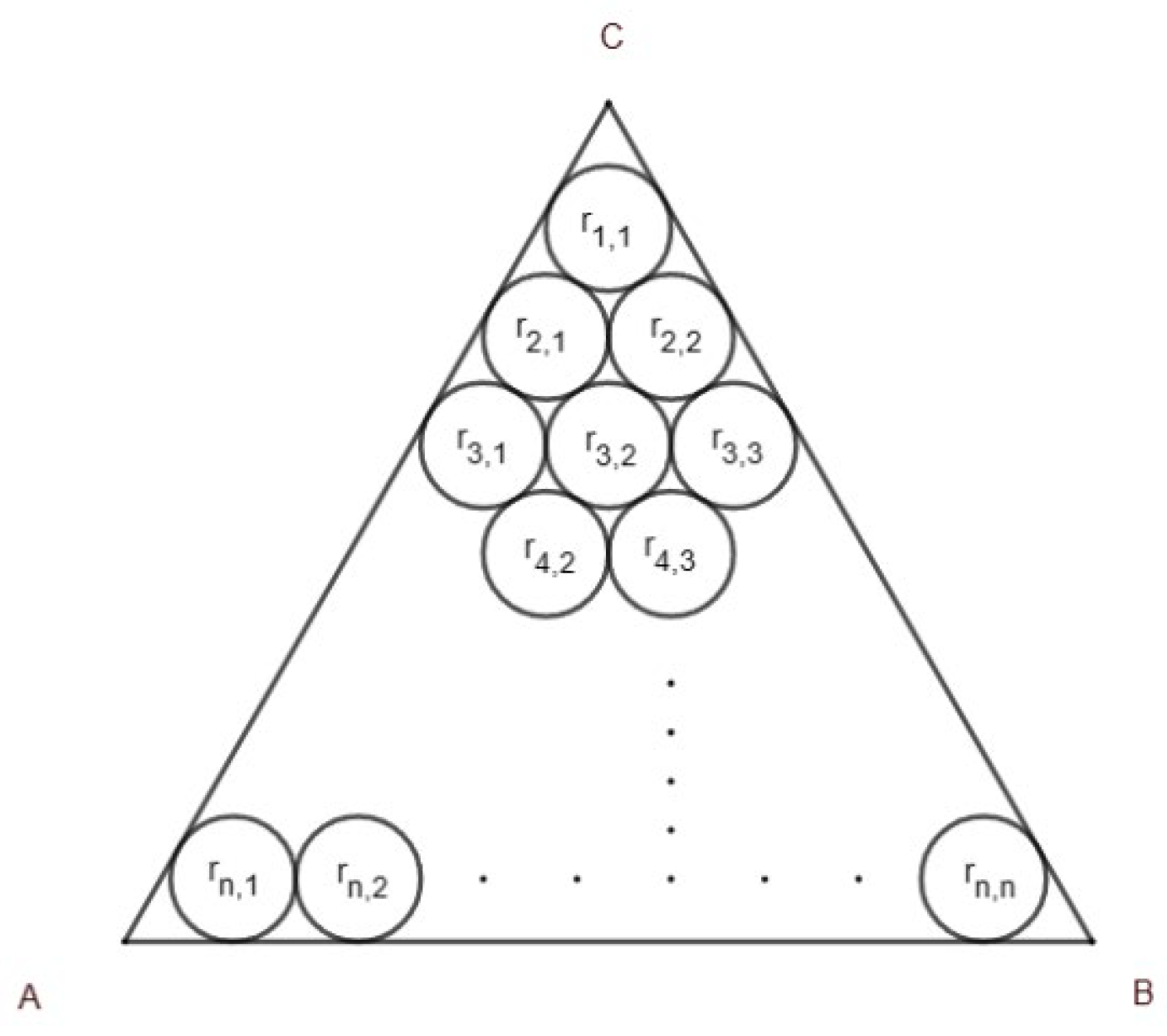
- Initial radius list r= [ri,j |where 1≤i≤n, 1≤j≤i.]
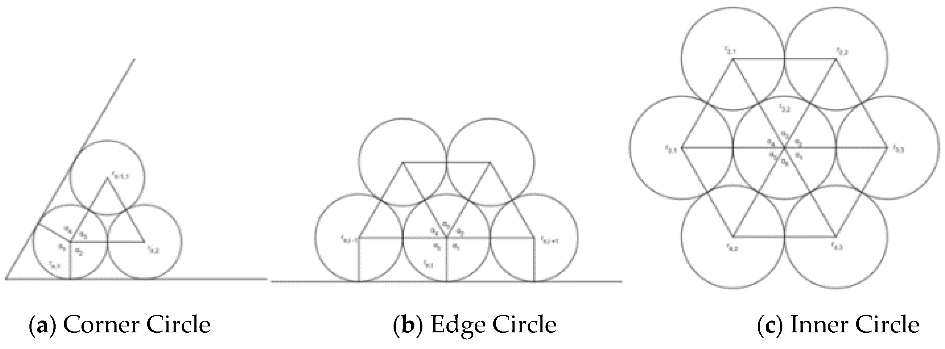
- Calculate the surrounding angle list for all circles Ci,j (whose associated radius is ri,j), call them θi,j.
-
While one of | θi,j-2π|>eps:
- 5.1
- Modify the radius list, all radii value is computed by current radii, and assign to new radius list in the meantime.
- 5.2
- Calculate the surrounding angle list for all circles Ci,j(using new radii), call them θi,j.
- 5.3
- From the radius list, calculate the change ratio, and modify the radius list from the change ratio.
- Display the result.
1.2. Problem Statement
2. Term, Theories and Algorithms
- 1.
- Input the coordinate of 3 vertices A, B, C; Calculate the angle A, B, C, and the edge length c.
- 2.
- Set a tolerance variable eps = 0.0001, epsr=0.3. Set a value r. set i=1.
- 3.
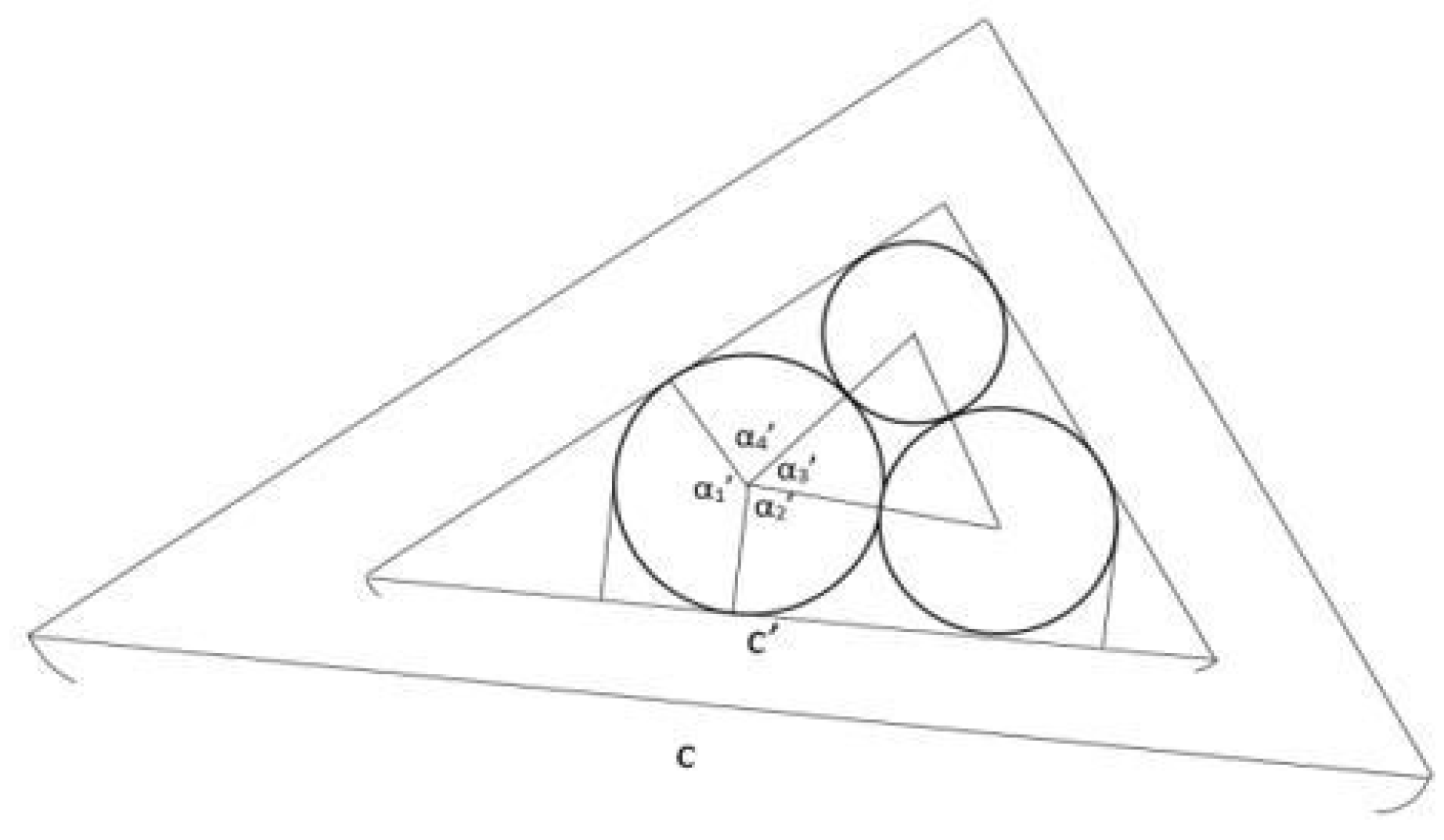
- Generate the r-offset of the triangle. Call it Ti.
- 3.1
- Generate the vertices on Ti.
- 3.2
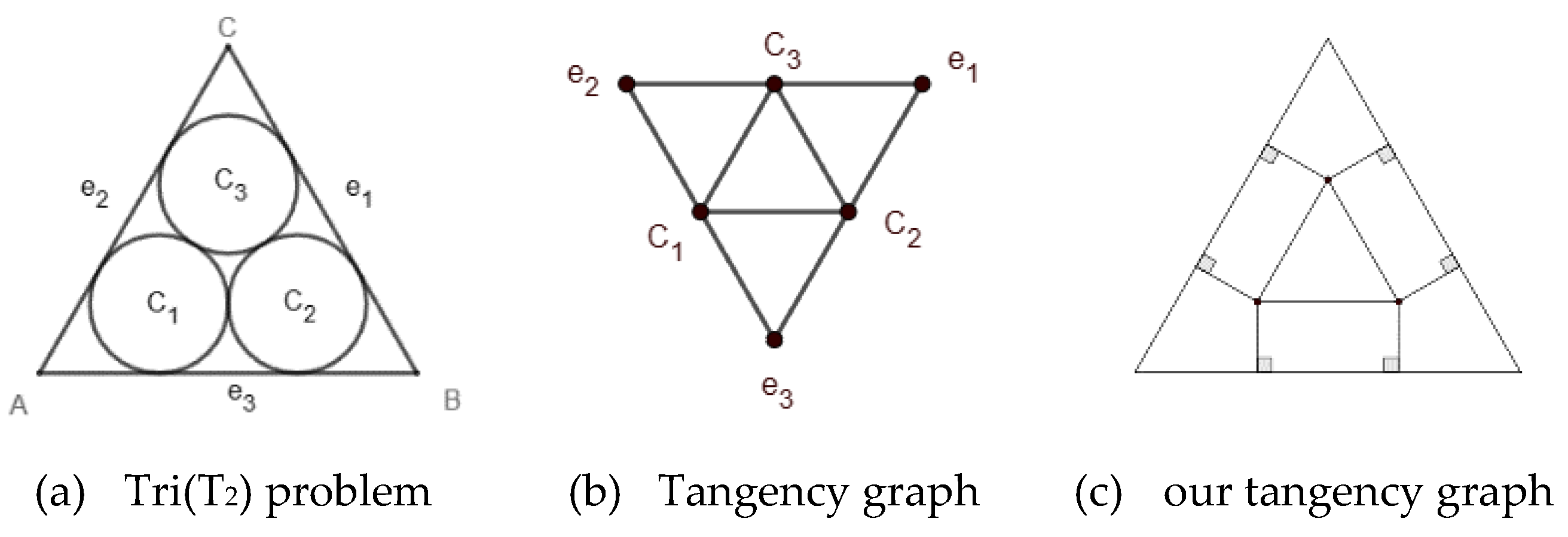
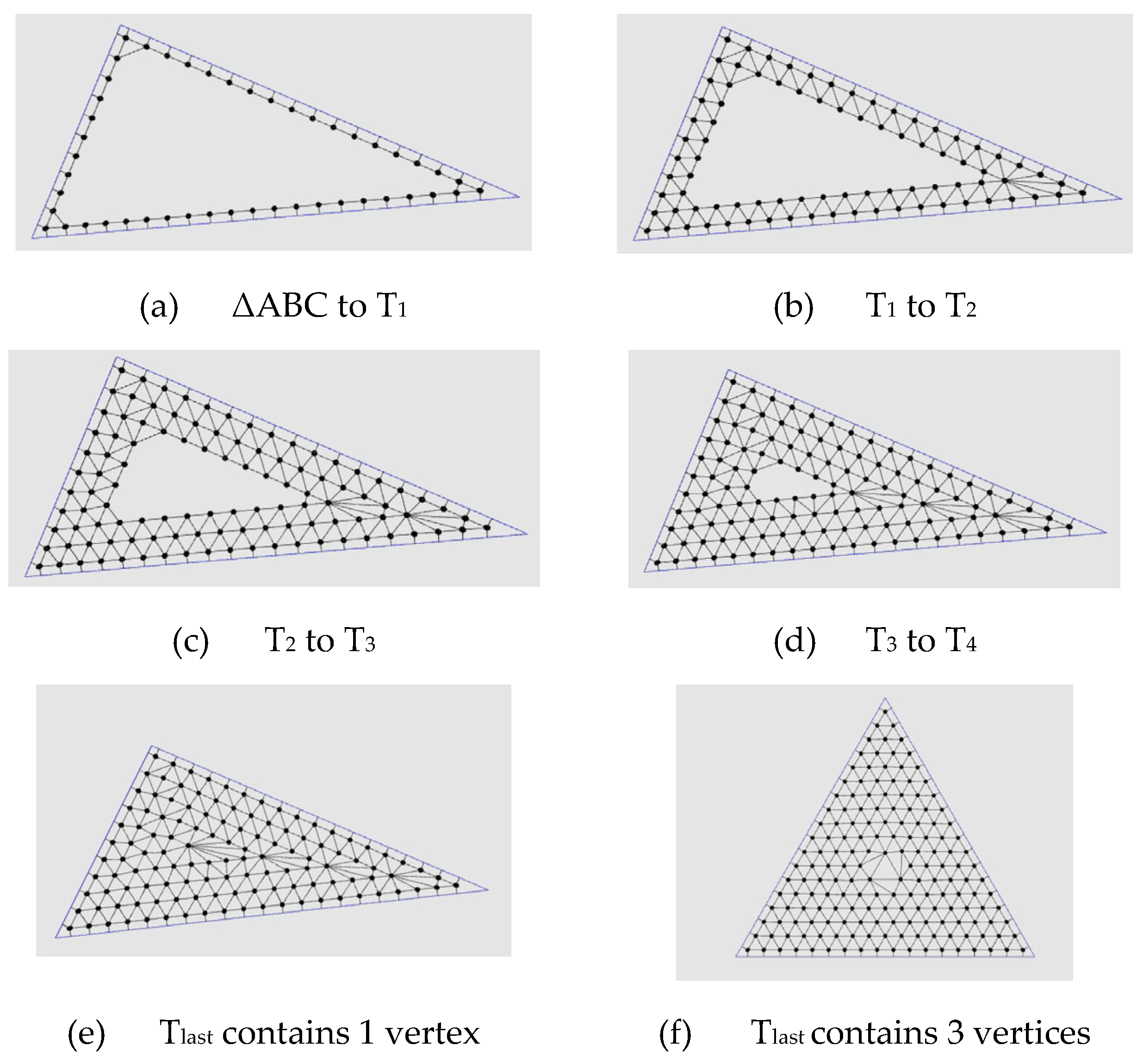
- Generate the edges for vertices on Ti, including the edges connecting 2 neighbors of vertices A, B, C. (See Figure 13a).
- 3.3
- Generate edges for vertices on Ti to the side of the triangle , , (See Figure 13a).
- 4
- While Ti did not satisfy some conditions:
- 4.1
- Generate the r-offset of the triangle Ti, call it Ti+1.
- 4.2
- Generate the vertices and edges on Ti+1, as we do on step 3.1 and 3.2.
- 4.3
- Generate the edge connect vertices on Ti to vertices on Ti+1. (See Figure 13b–f)
- 4.4
- i=i+1
- 5.
- Decide whether the last triangle contains only one vertex(circle) or 3 vertices(circles) (See Figure 13e,f. Call the last triangle Tlast.
- 6.
- Establish the edge of graph to connect Ti-1 and Tlast. (See Figure 13e,f)
- 7.
- Using Chiang’s algorithm with tolerance eps to find the solution.
- 8.
- Display the result.
- How to find the r-offset of a triangle in step 3
- How to construct the tangency graph (vertices and edges) for the same layer?
- How to construct the tangency (vertices and edges) for two consecutive layers?
- How the while loop stops in step 4.
2.1. Offset a Triangle
2.2. How to Construct Vertices and Edges on the Same Layer
- 1.
- The vertices of △A′B′C′ belongs to V.
- 2.
- For 3 sides of △A′B′C′:
- 2.1
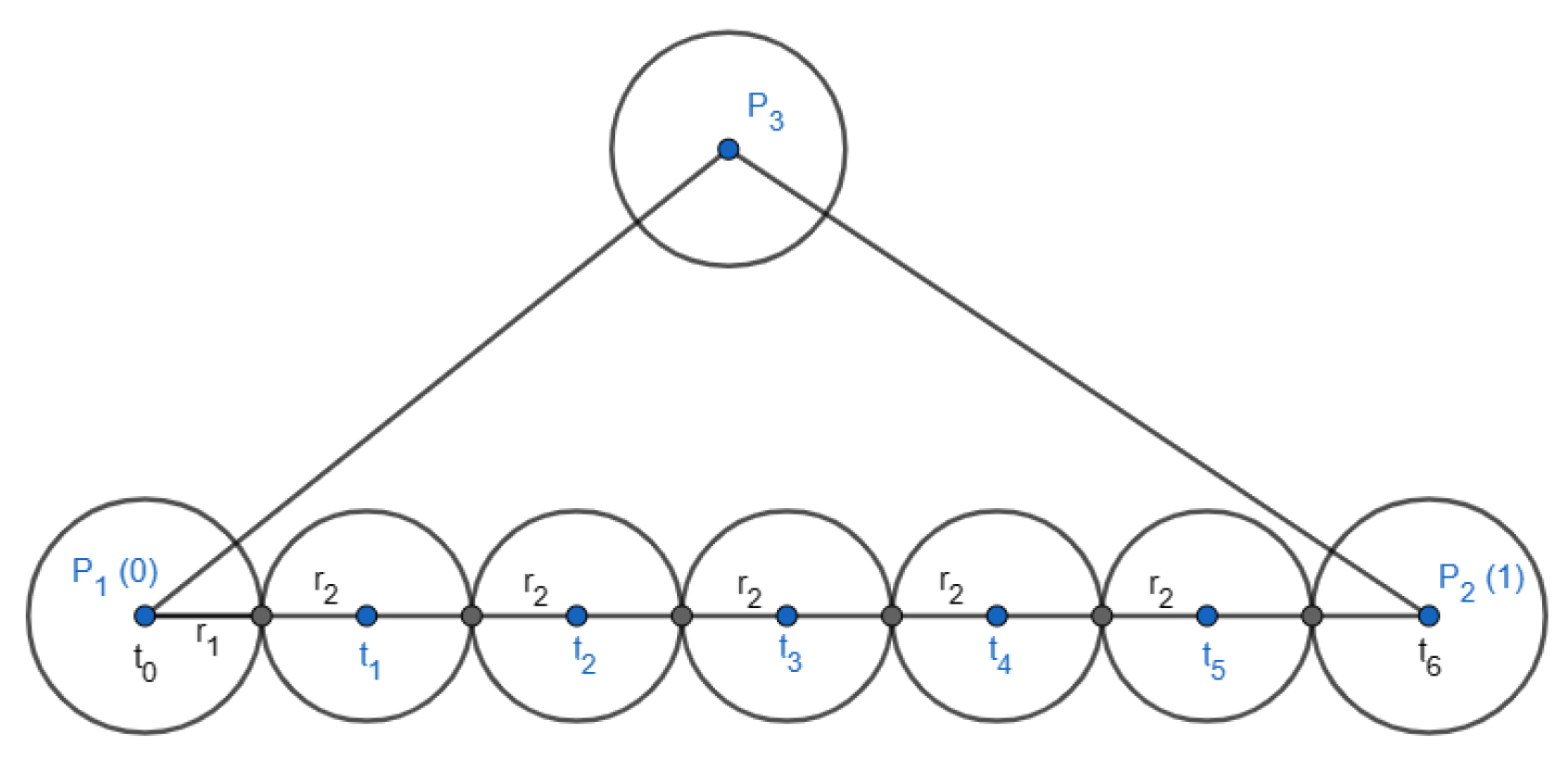
- Find the a value r′ and integer n, so that |r-r′| is minimum, and 2(r+n*r′) is equal to the length of this side of the △A′B′C′.
- 2.2
- From this r′, find associated vertices, which are center of a series of circles shown in Figure 12, in this side of triangle.
- 2.3
- Connect two consecutive vertices to establish edge of the graph.
- 3.
- Connect two neighbors of the vertices of △A′B′C′.
- 4.
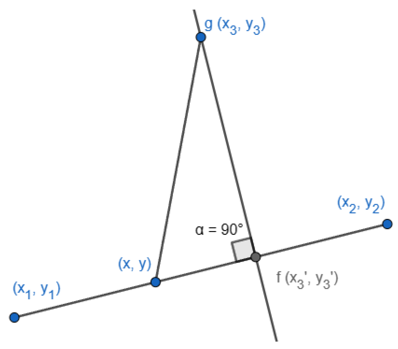
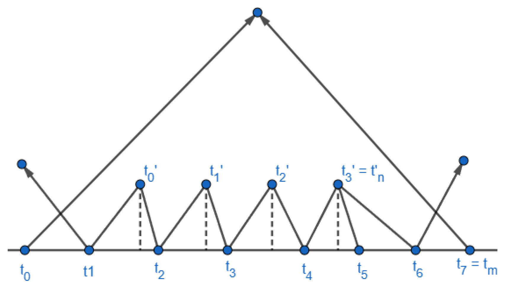
- Connect edges from to , from to , and from to (described in the section 2.3)
2.3. How to Construct Edges on Two Consecutive Layer
2.4. How to Stop the While Loop
3. Examples
4. Conclusions
Acknowledgments
References
- Malfatti, G. Memoria sopra un problema stereotomico. Memorie di Matematica e di Fisica della Società Italiana delle Scienze 1803, 10, 235–244. [Google Scholar]
- Chiang, C. S.; Hoffmann, C. M.; Rosen, P. A gereralized Malfatti’s Problem. Computational Geometry 2012, 45, 425–435. [Google Scholar] [CrossRef]
- Lob, H.; Richmond, H. W. On the Solutions of Malfatti's Problem for a Triangle. Proceedings of the London Mathematical Society 1930, s2-30, 287–304. [Google Scholar] [CrossRef]
- Wells, D. Malfatti's problem. In The Penguin Dictionary of Curious and Interesting Geometry; Penguin Books: New York, 1991; pp. 145–146. ISBN 978-0-14-011813-1. [Google Scholar]
- Ogilvy, C. S. Malfatti's problem. In Excursions in Geometry; Dover, 1990; pp. 145–147. ISBN 978-0-486-26530-8. [Google Scholar]
- Fukagawa, H. and Pedoe, D. "The Malfatti Problem." Japanese Temple Geometry Problems (San Gaku). Winnipeg: The Charles Babbage Research Centre, pp. 28 and 103-106, 1989.
- Bottema. The Malfatti Problem. Forum Geometricorum 2000, 1, 43–50. [Google Scholar]
- Stefanović, M. Triangle centers associated with the Malfatti circles. Forum Geometricorum 2003, 3, 83–93. [Google Scholar]
- Wolfram Math World. “Malfatti Circles,” Available online: http://mathworld.wolfram.com/MalfattiCircles.html.
- Ching-Shoei Chiang, Hung Chieh Li, Min-Hsuan Hsiung, and Fan-Ming Chiu. Extended General Malfatti’s Problem, The 19th International Conference on Scientific Computing, 2021/7/26-29.
- Weisstein, Eric W. "Line-Line Intersection." From MathWorld--A Wolfram Web Resource. Available online:. https://mathworld.wolfram.com/Line-LineIntersection.html.
- Collins, C. R.; Stephenson, K. A circle packing algorithm. Computational Geometry 2003, 25, 233–256. [Google Scholar] [CrossRef]

Disclaimer/Publisher’s Note: The statements, opinions and data contained in all publications are solely those of the individual author(s) and contributor(s) and not of MDPI and/or the editor(s). MDPI and/or the editor(s) disclaim responsibility for any injury to people or property resulting from any ideas, methods, instructions or products referred to in the content. |
© 2024 by the authors. Licensee MDPI, Basel, Switzerland. This article is an open access article distributed under the terms and conditions of the Creative Commons Attribution (CC BY) license (http://creativecommons.org/licenses/by/4.0/).


