Submitted:
11 July 2024
Posted:
12 July 2024
You are already at the latest version
Abstract
Keywords:
1. Introduction
2. Experimental Procedures
2.1. Experimental Materials and Treatment
2.2. Experimental Aging Solution
2.3. Experimental Device
2.4. Experimental Process
3. Results and Discussion
3.1. Microscopic Morphology Analysis
3.2. AE Parameter Analysis
3.3. Cluster Analysis
3.4. Least Squares Support Vector Machine Algorithm for Classified Prediction
4. Conclusions
Author Contributions
Funding
Acknowledgments
Conflicts of Interest
References
- Salibi, Z. Performance of reinforced thermosetting resin pipe systems in desalination applications: a long-term solution to corrosion — the Arabian Gulf example. Desalination 2001, 138, 379–384. [Google Scholar] [CrossRef]
- M. H N, Guihua H. Vinylester-glass fiber composite for water pipe: Processing and effect of fiber direction. Egyptian Journal of Petroleum 2023, 32, 24–30. [Google Scholar] [CrossRef]
- D. T L, Hassan K, Wayne H. Design of reinforced thermoplastic pipelines for hydrogen transport. Procedia Structural Integrity 2023, 45, 109–116. [Google Scholar] [CrossRef]
- Rodríguez, E.S.; Alvarez, V.A.; Montemartini, P.E. Failure analysis of a GFRP pipe for oil transport. Engineering Failure Analysis 2013, 28, 16–24. [Google Scholar] [CrossRef]
- Dandan, L.; Biao, H.; Jie, L.; et al. Failure analysis of glass fiber reinforced composite pipe for high pressure sewage transport. Engineering Failure Analysis 2023, 144. [Google Scholar]
- ZHANG Xuemin, LI Houbu, QI Dongtao, et al. Failure analysis of anticorrosion plastic alloy composite pipe used for oilfield gathering and transportation. Engineering Failure Analysis 2013, 32, 35–43. [Google Scholar] [CrossRef]
- W. B. Liau, F. P. Tseng. The effect of long-term ultraviolet light irradiation on polymer matrix composites. Polymer Composites, 1998; 440–445.
- L Monney, C Dubois, D Perreux, et al. Mechanical behaviour of an epoxy-glass composite under photo-oxidation. Polymer Degradation and Stability 1999, 63, 219–224. [Google Scholar] [CrossRef]
- Dionysis, E. Mouzakis, Helen Zoga, Costas Galiotis. Accelerated environmental ageing study of polyester/glass fiber reinforced composites (GFRPCs). Composites Part B 2006, 39, 467–475. [Google Scholar]
- Solis-Ramos, E.; Kumosa, M. Synergistic effects in stress corrosion cracking of glass reinforced polymer composites. Polymer Degradation and Stability 2016, 136, 146–157. [Google Scholar] [CrossRef]
- André, M.; Siguret, D.; Foulon, A.; et al. Corrosion evaluation of glass fiber reinforced plastic (gfrp) Tanks pressure vessels using acoustic emission technology. Synthèse: Revue des Sciences et de la Technologie 2019, 25, 129. [Google Scholar]
- Arumugam, V.; Kumar, C.S.; Santulli, C.; et al. Identification of Failure Modes in Composites from Clustered Acoustic Emission Data Using Pattern Recognition and Wavelet Transformation. Arabian Journal Forence & Engineering 2013, 38, 1087–1102. [Google Scholar]
- Wang, X.M.; Zhu, C.M.; Mao, H.L.; et al. Wavelet packet analysis for the propagation of acoustic emission signals across turbine runners. NDT&E International 2009, 42, 42–46. [Google Scholar]
- Dijck, G.V.; Hulle, M.V. Genetic algorithm for informative basis function selection from the wavelet packet decomposition with application to corrosion identification using acoustic emission. Chemometrics and Intelligent Laboratory System 2011, 107, 318–332. [Google Scholar] [CrossRef]
- Seif, E.H.; Alain, L.D.; Laurent, S.; et al. Acoustic emission pattern recognition approach based on Hilbert-Huang transform for structural health monitoring in polymer-composite materials. Applied Acoustics 2013, 74, 746–757. [Google Scholar]
- Pashmforoush, F.; Khamedi, R.; Fotouhi, M.; et al. Damage classification of sandwich composites using acoustic emission technique and k-means genetic algorithm. Journal of Technology & Science, 2014; 481. [Google Scholar]
- Momon, S.; Godin, N.; Reynaud, P. Unsupervised and supervised classification of AE data collected during fatigue test on CMC at high temperature. Compositespart A 2012, 43, 254–260. [Google Scholar] [CrossRef]
- Monti, A.; Mahi, E.A.; Jendli, Z.; et al. Mechanical behaviour and damage mechanisms analysis of a flax-fibre reinforced composite by acoustic emission. Composites Part A 2016, 90, 100–110. [Google Scholar] [CrossRef]
- Rolando, C.S.R.; Takenobu, S.; Shuichi, W. Analyzing the Sound of Materials: Application of Acoustic Emission Technique for Monitoring Material Behavior. Materials Science Forum 2024, 7136111–117. [Google Scholar]
- Claudia, B.; Caterina, C.; Giovanni, P.; et al. Laplacian score and K-means data clustering for damage characterization of adhesively bonded CFRP composites by means of acoustic emission technique. Applied Acoustics 2022, 185. [Google Scholar]
- Álvaro Carrasco, Franco Méndez, Félix Leaman, et al. Short Review of the Use of Acoustic Emissions for Detection and Monitoring of Cracks. Acoustics Australia 2021, 49, 1–8. [Google Scholar]
- Luigi, C.; Edoardo, P. A Review on the Applications of Acoustic Emission Technique in the Study of Stress Corrosion Cracking. Corrosion and Materials Degradation 2020, 2, 1–30. [Google Scholar]
- Zhang, Z.; Feng, H.; Zhao, W.; et al. Application of acoustic emission technology in hydraulic pressure test of nuclear power plant. IOP Conference Series: Earth and Environmental Science 2020, 514, 042039. [Google Scholar] [CrossRef]
- Zubova, M.E.; Tretyakova, V.T.; Wildemann, E.V. Application the acoustic emission technique to investigation of damage initiation in composites. Procedia Structural Integrity 2019, 18843–848. [Google Scholar] [CrossRef]
- Jing, N.J.; Dong, H.L.; Wang, D.H.; et al. Application of Acoustic Emission Technology for Quantitative Characterization of Plasma-Sprayed Coatings Subjected to Bending Fatigue Tests. Journal of Thermal Spray Technology 2018, 27, 1090–1102. [Google Scholar] [CrossRef]
- Tayfur, S.; Alver, N.; Abdi, S.; et al. Characterization of concrete matrix/steel fiber de-bonding in an SFRC beam: Principal component analysis and k -mean algorithm for clustering AE data. Engineering Fracture Mechanics 2018, 19473–85. [Google Scholar] [CrossRef]
- Shenglan, M.; Shurong, R.; Zhining, C.; et al. Wooden beam damage evaluation under bending loading based on the integration of acoustic emission and principal component analysis. Measurement 2023, 222. [Google Scholar]
- Suykens, J.A.K.; Vandewalle, J. Least Squares Support Vector Machine Classifiers. Neural Processing Letters 1999, 9, 293–300. [Google Scholar] [CrossRef]
- Xi, P.; Zhao, Y.; Wang, P.; et al. Least squares support vector machine for class imbalance learning and their applications to fault detection of aircraft engine. Aerospace Science and Technology 2019, 8456–74. [Google Scholar] [CrossRef]
- Jiankai Xue. Research and Application of A Novel Swarm Intelligence Optimization Technique: Sparrow Search Algorithm. Master’s Degree, Donghua University, Shanghai, 2020.


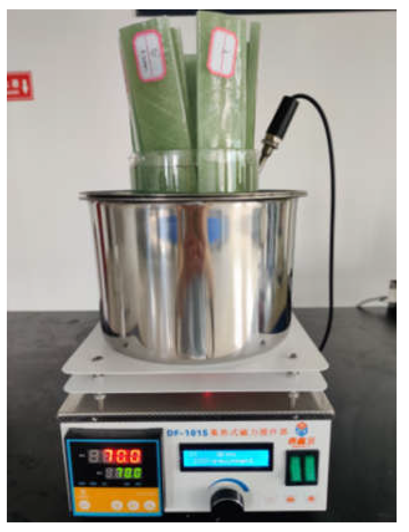
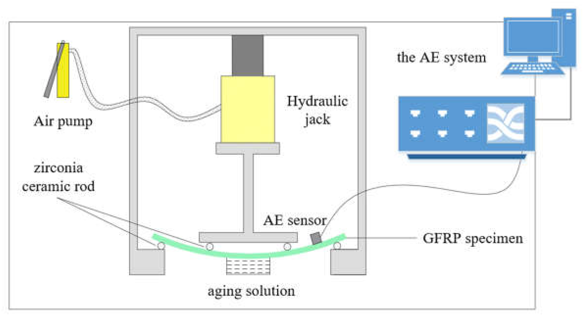
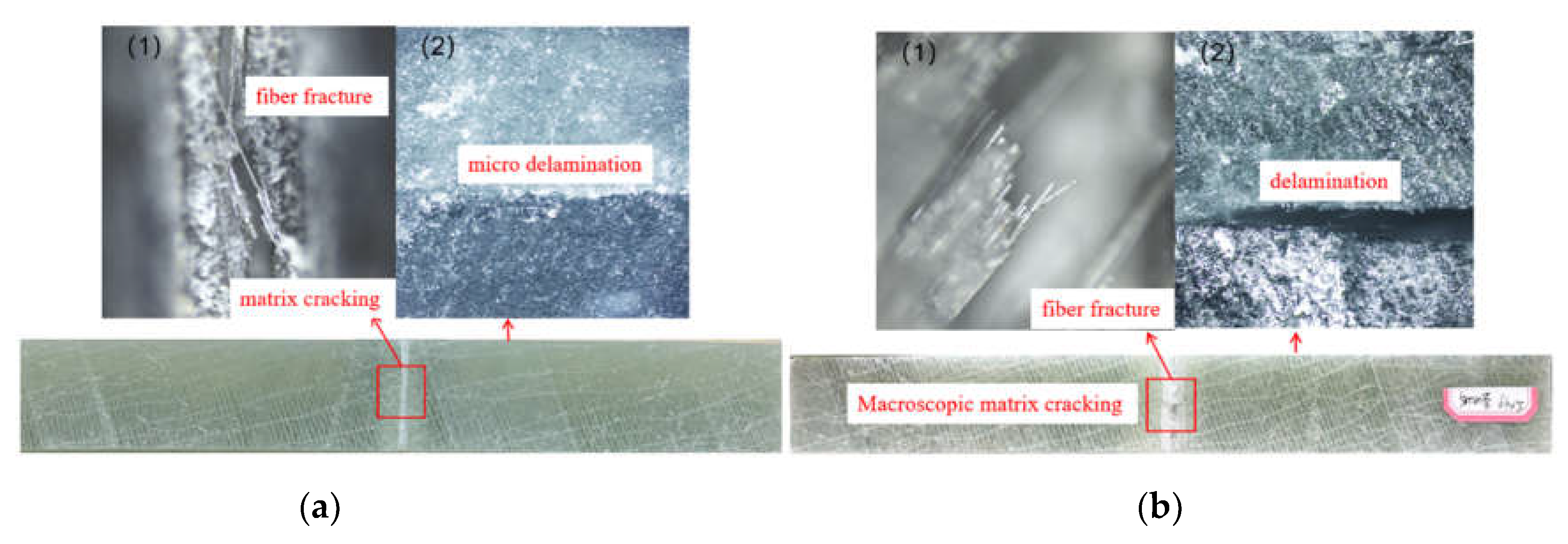
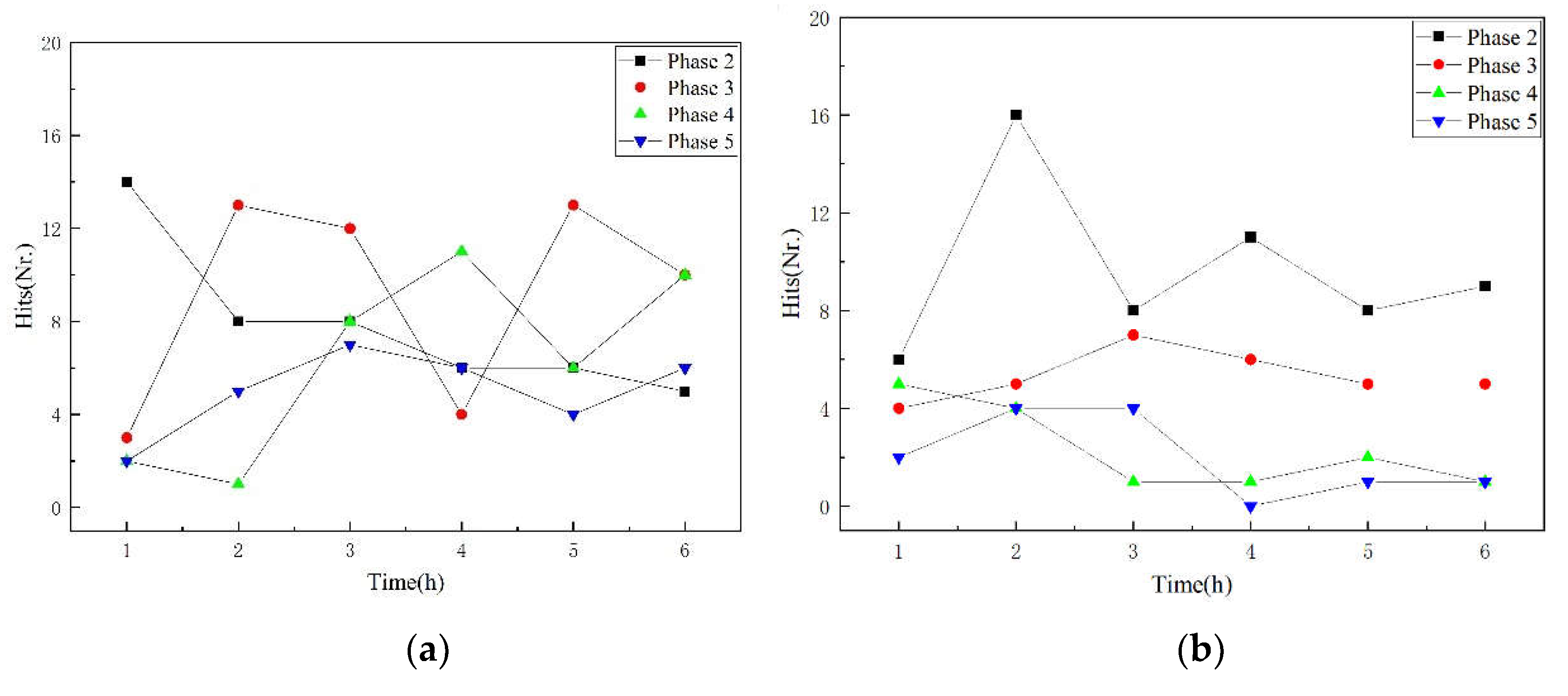
| angle | thickness | ||
|---|---|---|---|
| winding angle | inner liner | inner winding layer | outer winding layer |
| 54.75° | 3mm | 3mm | 1.5mm |
| ion | Cl- | HCO3- | Ca2+ | Mg2+ |
|---|---|---|---|---|
| concentration (g/L) | 15 | 0.8 | 0.8 | 0.8 |
| preprocessed specimens | Specimen number | Degree of damage |
|---|---|---|
| 2mm | A1 | Matrix crack |
| 5mm | A2 | Obvious delamination |
| damage type | Hits | |||
| matrix cracking | debonding | delamination | fiber fracture | |
| A1 | 9676 | 21621 | 2863 | 77 |
| A2 | 162 | 457 | 170 | 17 |
| damage type | Hits | ||
| matrix crack | debonding | delamination | |
| A1 | 99 | 37 | 34 34 |
| A2 | 8 | 47 | |
| Model | Experimental stage | Sample number of training set | Sample number of the testing set |
|---|---|---|---|
| Model 1 | Stress damage stage | 350 | 110 |
| Model 2 | Aging stage | 100 | 50 |
Disclaimer/Publisher’s Note: The statements, opinions and data contained in all publications are solely those of the individual author(s) and contributor(s) and not of MDPI and/or the editor(s). MDPI and/or the editor(s) disclaim responsibility for any injury to people or property resulting from any ideas, methods, instructions or products referred to in the content. |
© 2024 by the authors. Licensee MDPI, Basel, Switzerland. This article is an open access article distributed under the terms and conditions of the Creative Commons Attribution (CC BY) license (http://creativecommons.org/licenses/by/4.0/).


