1. Introduction
The analysis of products on store shelves has been a research focus for decades [
1,
2,
3,
4,
5,
6,
7,
8,
9,
10,
11,
12]. Recognizing individual products at the SKU (Stock Keeping Unit) level can enhance sales processes, assist disabled individuals, and facilitate sales analysis of store shelves. A significant challenge in this area is the diversity of products, the vast number of classes, frequent packaging changes, and seasonal rotations, all of which demand flexible and scalable solutions. Typically, automated SKU recognition involves two stages: detecting the products on the shelf and then recognizing them. While state-of-the-art detectors effectively detect products [
13], the recognition problem remains challenging [
14].
Advanced machine learning techniques, such as deep convolutional neural networks, are not feasible for this problem due to the continuous rotation of products and the large number of classes, which complicate model retraining. Therefore, recognition methods often focus on generating multidimensional embedding vectors that compare the encoded features of detected products with the patterns stored in a database. However, creating a pattern set that accounts for different views of each product, varying lighting conditions, noise, or color temperature is nearly impossible. Thus, SKU recognition should be approached as a one-shot or few-shot learning problem, where the goal is to infer the class of a detected product based on one or a few prototype images. Given that every product launched on the market initially has a digital design of its label/facing or an e-commerce model used in online store listings, a recognition process based on such a single prototype would be groundbreaking.
To address these challenges, this paper explores the potential of one-shot learning, which relies on a single prototype image per class and is particularly suited for environments where data scarcity is the norm. We introduce and evaluate the VPE (Variational Prototyping Encoder) architecture for classifying store-shelf products. The VPE architecture effectively handles domain discrepancies and data imbalances by utilizing pairs of prototype and real images [
15]. This approach facilitates the learning of latent feature space, where a variational autoencoder (VAE) ensures that features of actual products are tightly clustered around the prototype features.
The main contributions of this paper can be summarized as follows:
the Variational Prototyping Encoder (VPE) was adapted for product recognition on retail shelves,
various loss functions in the Variational Autoencoder (VAE) model were analyzed to enhance performance,
the cosine metric was introduced to the nearest neighbor method to improve similarity measurement,
the method was modified by incorporating prototypes as a signal at the encoder input,
tests were conducted to select suitable prototypes for different classes,
background removal and size uniformity were applied to prototypes and extracted products to optimize the recognition process and eliminate irrelevant disturbances,
the optimal network parameters and latent space size were tested and selected to ensure effective performance.
2. Related Works
One-shot learning stands out as a pivotal technique where a model is designed to acquire knowledge from a single example, contrasting sharply with traditional deep learning approaches that rely on extensive datasets. Pioneering efforts in this field, such as the work of Li et al., utilize a Bayesian strategy to harness latent and generic prior information, demonstrating that such learned priors can adapt effectively to various small-data problems, thereby alleviating issues of data imbalance and showing promising generalizability [
16]. Furthering these concepts, Lake et al. explored the generative processes using hierarchical Bayesian models, which proved capable of extending to new tasks with minimal data input [
17].
Recent strategies in one-shot learning have focused on embedding learning and meta-learning. Works by researchers [
18,
19] have advanced the field of metric learning by transforming task-related information into a metric space where classification occurs through the comparison of similarity scores. In contrast, approaches by [
20,
21] aim to imbue models with the ability to adapt to new tasks, aligning with meta-learning methodologies.
Chen et al. [
22] have extended prototype learning to one-shot image segmentation by incorporating multi-class label information during episodic training to generate more nuanced feature representations for each category. Prototypical Networks [
23] introduced an approach where classification in few-shot scenarios is facilitated by computing distances to class-centered prototypes, representing a simpler yet effective bias beneficial in limited-data conditions.
When addressing the challenges of retail shelf product recognition, Wang’s proposal of an enhanced Siamese neural network in one-shot learning is particularly noteworthy [
24]. This approach introduces a spatial channel dual attention mechanism aimed at refining the network architecture, significantly enhancing the network’s ability to focus on and interpret subtle product details.
On the generative modeling front, variational Autoencoder (VAE), introduced by Kingma and Welling, is a generative model comprising encoder and de-coder networks [
25]. VAE encodes input data into a latent space and decodes it back to the original domain, facilitating tasks like image reconstruction and generation. Variational Prototyping Encoder (VPE), a derivative of VAE, presented by Kim et al., specializes in the one-shot classification of graphic symbols, enabling categorization with a single prototype image per class [
15].
Recent research explores extensions like Variational Multi-Prototype Encoder (VaMPE) [
26] or Semi-Supervised Variational Prototyping Encoder (SS-VPE) [
27]. VaMPE utilizes multiple prototypes per class to enhance model performance without the need for additional sub-labeling. SS-VPE employs generative unsupervised learning to optimize prototypes in latent space, applies a Student’s-t mixture model for robust outlier management, and advances the VAE for enhanced few-shot semi-supervised learning performance. It’s also worth mentioning the introduction of VPE++, which inherently reduces hubness and incorporates contrastive and multi-task losses to increase the discriminative ability of few-shot learning models [
28].
The evolving landscape of one-shot learning, prototype methods, and VAE-based approaches underscores the continuous efforts to address challenges in learning from limited data and improve the efficiency and effectiveness of machine learning models. These advancements hold promise for applications across various domains, including image recognition.
This paper focuses on employing one-shot learning techniques utilizing prototype SKU images. One-shot learning, which trains a model to recognize patterns or objects with a single example, makes it particularly suited for scenarios with limited data. Here, prototypes, representative examples of product categories, are utilized alongside unique Stock Keeping Unit (SKU) identifiers to develop a model capable of discerning various products from single instances.
3. Method
This section describes the Variational Prototyping Encoder (VPE) proposed in [
15] adopted to SKU recognition case.
3.1. Variational Prototyping Encoder
The Variational Prototyping Encoder is established through the derivation of the marginal likelihood concerning the input data, denoted as
x. Its lower bound characterizes the self-expression of the input, as depicted by the equation:
where
x is the real image sample,
t denotes its corresponding prototype image. A latent code
is sampled from a prior distribution
, followed by the generation of a prototype
from a conditional distribution
. The Kullback-Leibler (KL) divergence denoted as
is employed here, alongside a proposal distribution
, which serves to approximate the inherently intractable true posterior. These distributions, namely
and
, are commonly referred to as a probabilistic encoder and decoder, or alternatively as a recognition model and a generative model. The parameters
and
correspondingly represent the parameters of the encoder and decoder.
In this model, x undergoes encoding into z and subsequent reconstruction from z. However, the approach covered in this article extends beyond this paradigm by encoding the input x into z and translating it to a prototype, analogous to image-to-image translation. Unlike typical reconstructions, prototypes exist within a canonical domain with standardized colors, devoid of real-world perturbations commonly found in physical objects.
The described method serves to translate real image inputs into corresponding prototypical images that remain invariant despite real-world perturbations such as background clutter, geometric variations, and photometric alterations. In essence, VPE exhibits parallels with the denoising autoencoder, functioning as a normalization mechanism for real-world perturbations. Consequently, VPE has the potential to generate latent embeddings z, that are either invariant or robust in the face of such perturbations.
3.2. Training and Testing Phases
In the Variational Prototyping Encoder, two primary phases can be delineated.: the training and testing stages. During the training phase
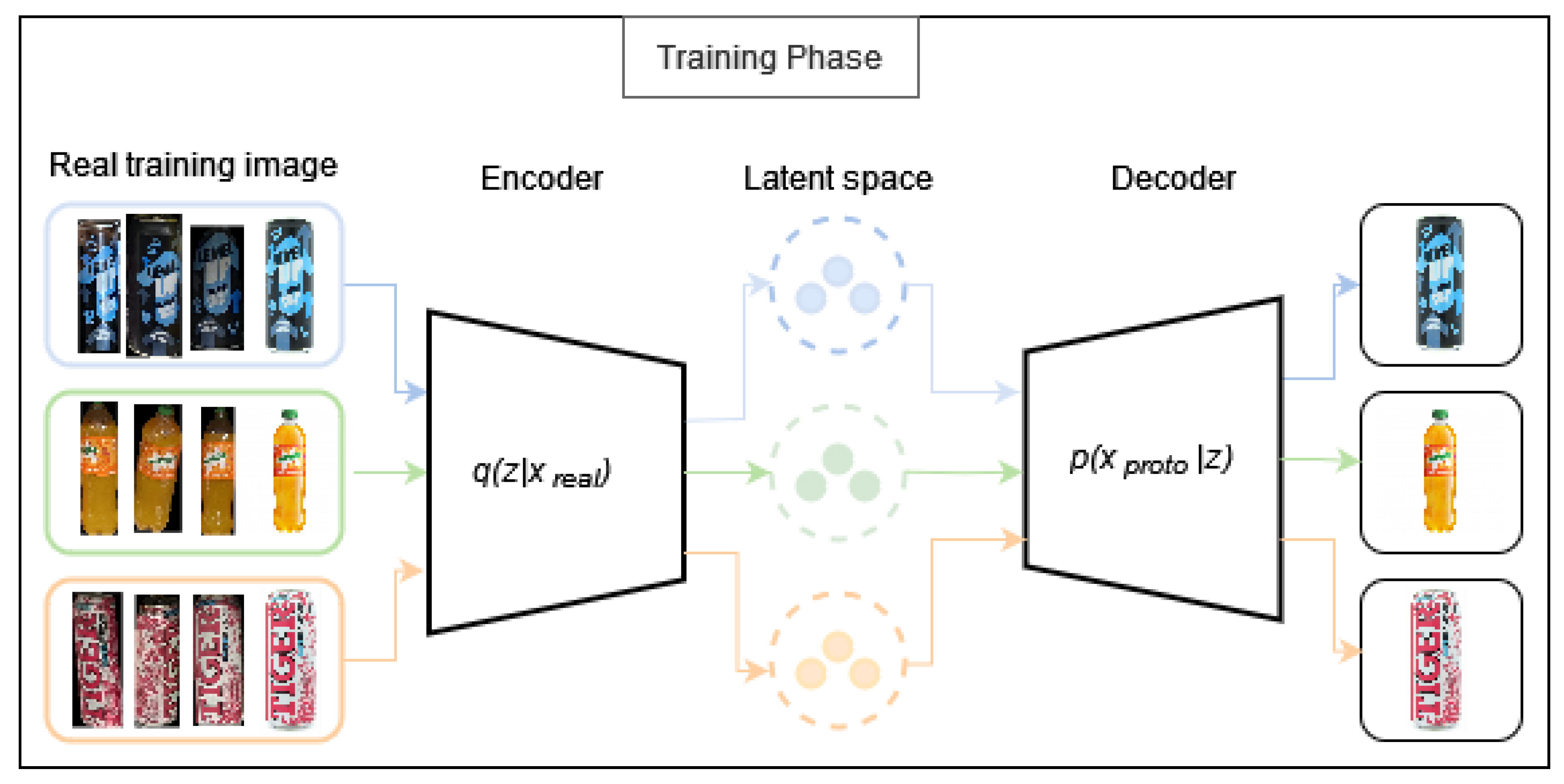
Figure 1, the encoder transforms input images from the real domain into a latent distribution denoted as
. Furthermore, in this research, prototypes are included alongside real training images as inputs to the encoder, significantly enhancing the results achieved. Consequently, the prototype becomes a potent signal. Subsequently, the decoder reconstructs the encoded distribution into a prototype corresponding to the input image. In the testing phase
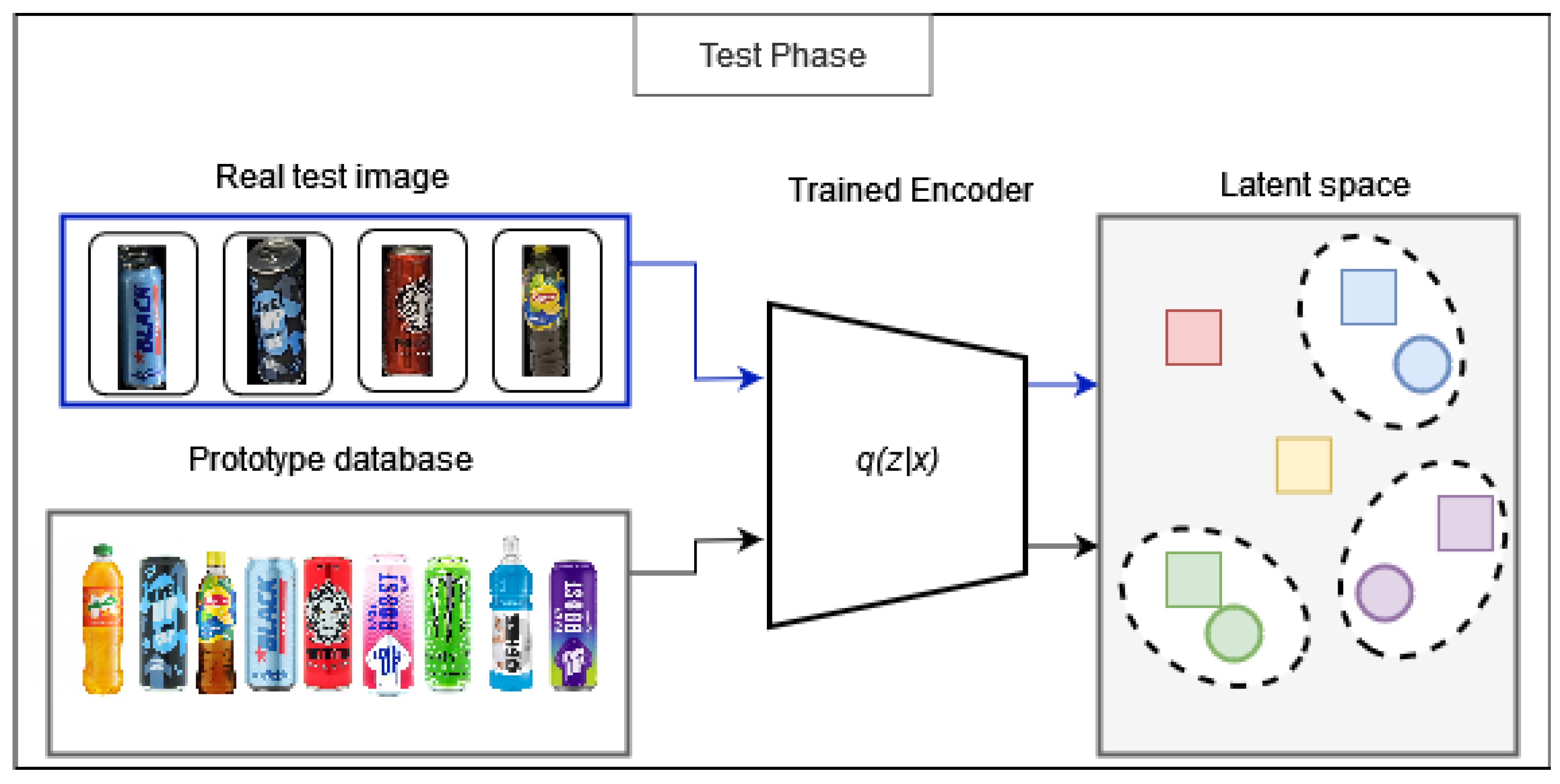
Figure 2, the trained encoder serves as a feature extractor. Both test images and prototypes from the database undergo encoding into the latent space. Subsequently, nearest neighbor classification is performed to categorize the test images. Additionally, during the training phase, the model’s performance is evaluated using a validation set, allowing for the assessment of its effectiveness throughout the training process.
It’s essential to note that the testing is conducted on previously unseen images from classes already encountered, as well as entirely new classes for the encoder.
3.3. Network Architecture
An encoder was built with three convolution layers, each followed by a fully connected layer for mean and variance predictions. A stride size of 2 was used for each convolution layer, downsizing the feature map by a factor of 2. Batch normalization and leaky ReLU were applied after every convolution layer. The final layer consisted of a fully connected layer converting a feature map into a predefined latent variable size.
The decoder’s layers were arranged inversely to the encoder’s, with a fully connected layer followed by three convolution layers. Before each convolution, upsampling by a factor of 2 was performed to recover the feature size to the original input dimensions. All convolution kernels in the decoder were set to . Similar to the encoder, batch normalization, and leaky ReLU were applied after every convolution operation.
3.4. Loss Functions
Various loss functions for Variational Prototyping Encoders were implemented and tested. The following were included:
4. Experiments
4.1. Dataset Overview
The research consisted of two phases. In the first phase, a dataset was created by extracting products from store shelf photos, specifically designed to include non-alcoholic beverages, both canned and bottled variants. The images were taken within stores belonging to one of the most numerous retail chains in Poland, and canned products are prevalent due to the specific nature of the store. To enhance the robustness and variability of the dataset, photos were captured under various conditions—different angles, lighting, and distances—ensuring a comprehensive representation of real-world scenarios. Each product was then extracted and categorized, creating a structured dataset tailored for the evaluation of our one-shot learning model. The dataset is partitioned into three subsets: a training set, a validation set, and a test set. The training set consists of samples from 38 distinct classes, while the validation set encompasses 11 classes. The test set consists of 15 classes, further divided into two categories: ’seen’ and ’unseen’ classes. The ’seen’ subset comprises 6 classes, representing classes that the model has been exposed to during the training process, although the specific photos in this subset have not been seen by the model. Conversely, the ’unseen’ subset contains 9 classes that are entirely novel to the model and not encountered during the training phase.
In the second phase, a dataset representing products from store shelves was created using frames extracted from video recordings. This introduced the additional challenge of recognizing products from lower-quality images. The dataset includes all products available in popular franchise stores, categorized by SKU, which accounts for factors such as product size. The research focused on beverages (1070 classes), dairy products (270 classes), and snacks (156 classes), which constitute the majority of the store’s inventory. The dataset was also divided into training, validation, and test sets in a 70:15:15 ratio.
This dataset structure facilitates rigorous evaluation of the model’s performance across various scenarios, including its ability to generalize to unseen classes, thus providing insights into its robustness and efficacy in real-world applications.
4.2. Implementation Overview
During the course of the research, various optimizers and parameter values were rigorously tested to determine the most effective settings for training the networks. Ultimately, the ADAM optimizer was selected for its robust performance, with a learning rate finely tuned to , beta values set at (0.9, 0.999), an epsilon value of , and a mini-batch size of 154. The effects of different image resolutions were also investigated, leading to an adaptation in the input dimension of the initial fully connected layer, which adjusts dynamically based on the input size. As a result of the tests that were conducted, it was demonstrated that higher values for the convolution filter size and latent variable size yield better results. Therefore, it was decided to set the convolution filter sizes at [200, 250, 350] and the latent variable size at 600. Moreover, the architecture has been significantly improved by the strategic integration of spatial transformer modules into the encoder part. These modules are positioned before the 1st and 3rd convolution layers to enhance spatial invariance.
4.3. Results
Based on the conducted experiments, it was decided to modify the algorithm by adding prototypes to each training set, as a significant increase in recall for unseen classes, from 0.686 to 0.922, was observed.
A comparison of recall metrics obtained through different evaluation methods and distance measures was conducted and presented in
Table 1. Two distance measures, Euclidean and Cosine, are evaluated. For the Euclidean distance measure, when the recall is calculated after a specified number of epochs, the results show that for all instances, the recall is 0.888, while for the training set, it’s 0.894, and for the test set, it’s 0.883. In terms of top-nn recall, for second nearest neighbors (2-nn), it achieves 0.972, and for third nearest neighbors (3-nn), it’s 0.986. However, when recall is triggered by validation, the overall recall decreases to 0.769, with 0.939 for the training set and a significant drop to 0.623 for the test set. The top-nn recall also declines to 0.825 for 2-nn and 0.839 for 3-nn. Conversely, for the Cosine distance measure, recall values are consistently higher. When evaluated after a specified number of epochs, the overall recall is 0.916, with 0.909 for the training set and 0.922 for the test set. The top-nn recall is notably high, reaching 0.986 for 2-nn and 0.993 for 3-nn. Similarly, when recall is triggered by validation, the overall recall remains relatively high at 0.888, with 0.955 for the training set and 0.831 for the test set. The top-nn recall maintains its high values at 0.986 or 0.993 for both 2-nn and 3-nn. These results suggest that the Cosine distance measure consistently outperforms the Euclidean measure across both evaluation methods, yielding higher recall values across all scenarios.
For the VPE algorithm applied to image sizes of
pixels
Table 2: Mostly, the model achieves high recall for seen classes, ranging from 0.939 to 0.955 and for unseen classes from 0.896 to 0.961. However, its performance decreases to 0.576 for seen classes, when rotation as augmentation technique is applied. The addition of augmentation or stn (spatial transformer attached to the encoder part- tor the stn version, the spatial transformer modules are applied before the 1st and 3rd convolution layers in the encoder part) slightly affects recall for both seen and unseen classes.
For the same algorithm applied to image sizes of
pixels
Table 2: The model maintains relatively high accuracy for seen classes, ranging from 0.924 to 0.970. However, performance on unseen classes varies, with augmentation techniques generally improving accuracy, except when rotation is applied. This may be due to the fact that beverages on shelves usually have a fixed, vertical position.
Overall, the differences in performance based on image size exist. However, by employing appropriate techniques for both investigated sizes, high recall can be achieved.
In this study, various loss functions were tested to evaluate their performance in the context of Variational Prototyping Encoder problems
Table 3. The selected loss functions are as follows: sum of two components: Binary Cross Entropy (BCE) and Kullback-Leibler Divergence (KLD), Relative Average Spectral Error (RASE), Root Mean Square Error (RMSE) and Relative Dimensionless Global Error in Synthesis (ERGAS). Ultimately, each of the applied loss functions allowed for achieving very high performance, confirming their effectiveness in the context of variational autoencoder analysis.
A comparison of results for various prototypes within a single class was conducted. Images depicting the product rotated at different angles were tested to define and ultimately select the prototype most suited to real-world conditions
Figure 3.
The background of all prototypes was standardized to black to match the backgrounds present in all images depicting the extracted product. This was accomplished with the help of The Segment Anything Model, a cutting-edge image segmentation model that allows for promptable segmentation, delivering unmatched versatility for tasks involving image analysis [
30].
In our study, the model demonstrates satisfactory performance, as indicated by the metrics of recall, accuracy, and precision
Table 4. Recall, defined as the ratio of true positives to the sum of true positives and false negatives, showcases the model’s ability to correctly identify instances of a particular class. Accuracy, calculated as the ratio of the sum of true positives and true negatives to the total number of instances, reflects the overall correctness of the model’s classifications. Precision, which is the ratio of true positives to the sum of true positives and false positives, measures the model’s ability to correctly classify instances as positive. While the model exhibits better performance for seen classes, the differences are marginal.
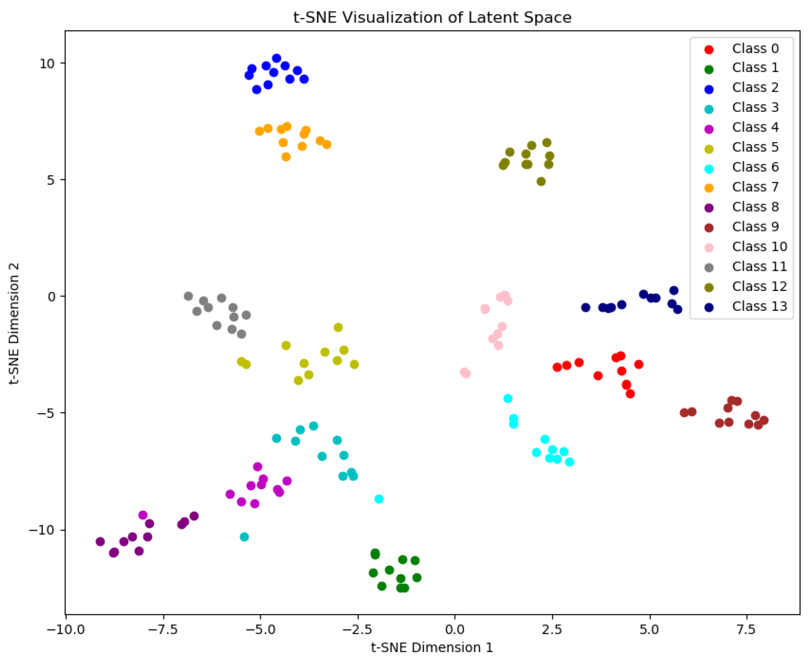
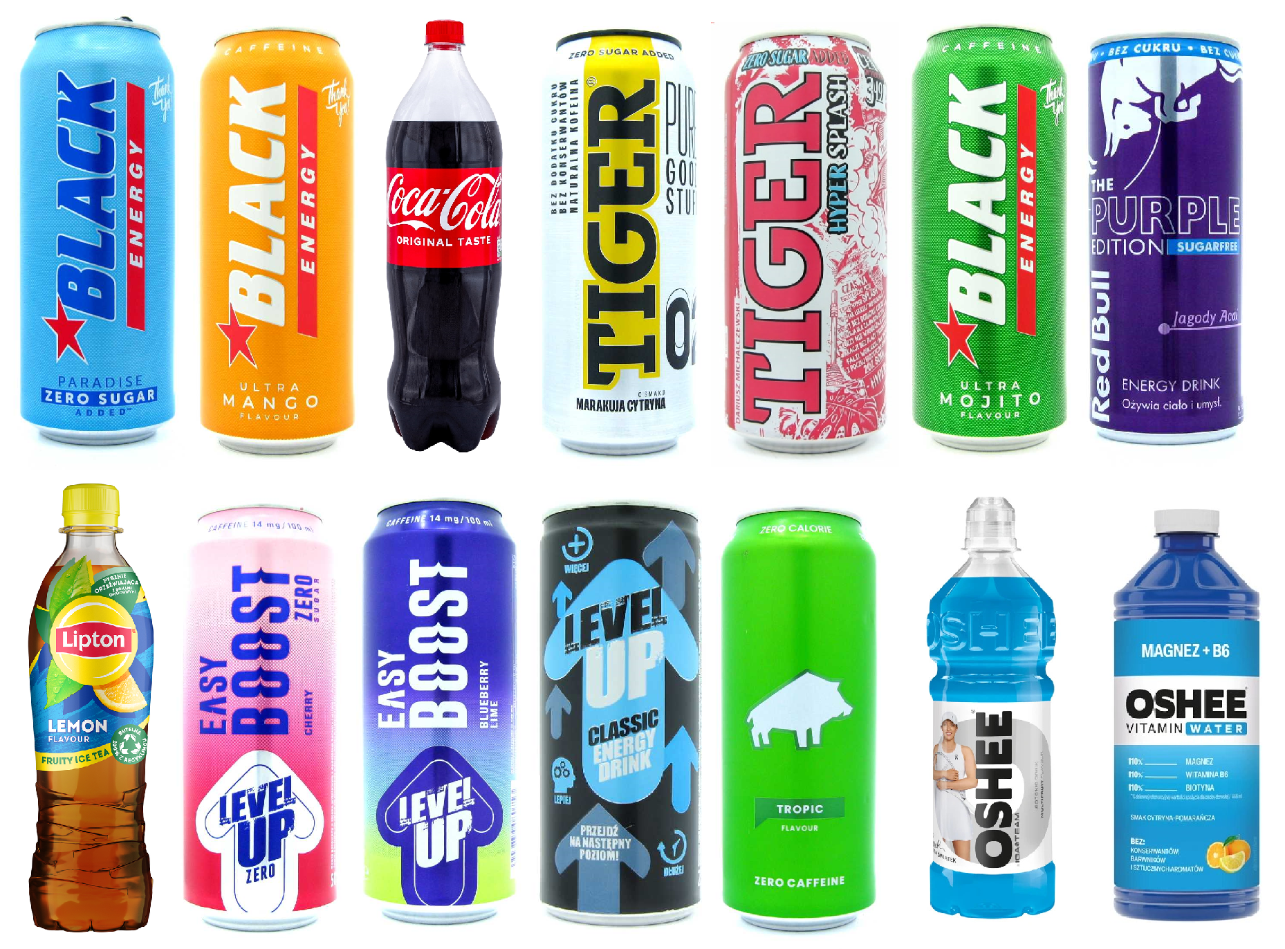
Figure 4 illustrates clearly defined clusters of objects of each class from the test set
Figure 5, indicating that the points corresponding to a specific class are close to each other.
In the second phase of the study, a dataset was used that was derived from frames extracted from video recordings. The performance of the algorithm was compared across products from different categories, demonstrating that certain categories, such as snacks, are easier to recognize than others, such as dairy products
Table 5. Dairy products tend to be smaller, and their significant identifying features are often located not only on the front of the packaging but also on the lids. Additionally, the labels of dairy products frequently use muted, similar colors.
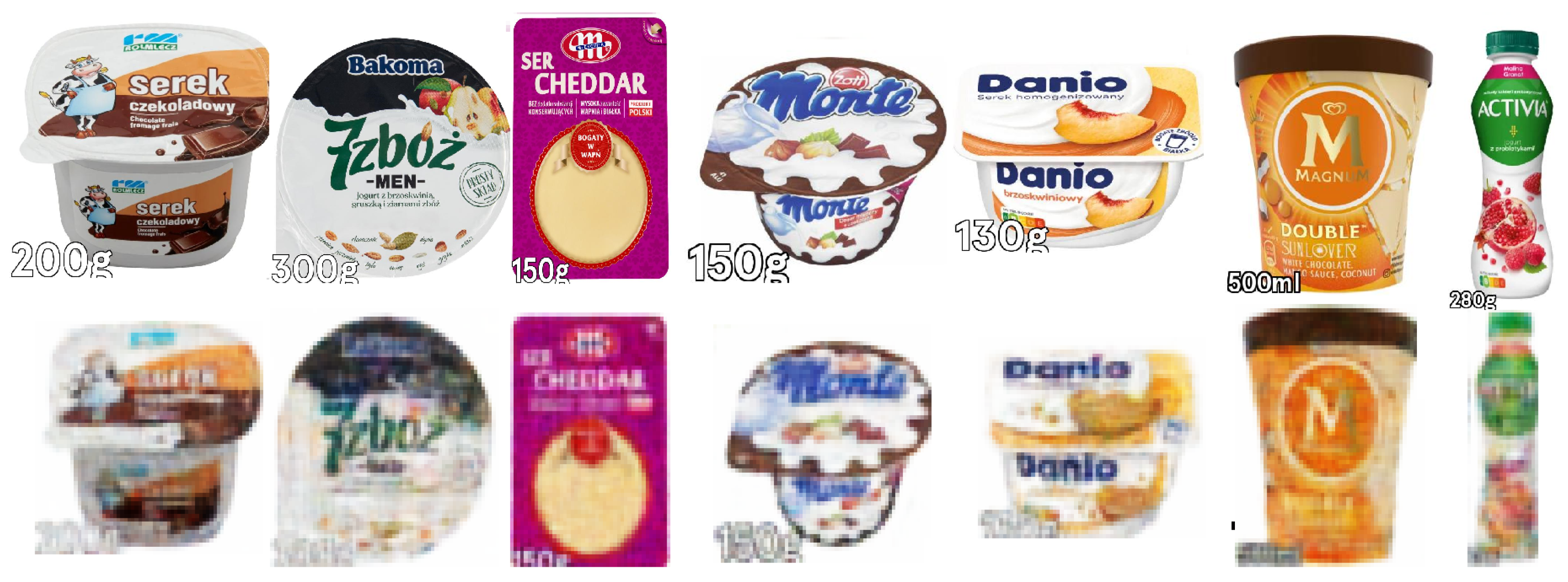
The model performs very well with images of classes that it encountered during the training phase. It is important to note that the images of seen classes used in the test set are from other video recordings, which the model had not previously seen in the training phase. The model can effortlessly distinguish visually similar products of the same brands with similar packaging, differing only in aspects such as flavor, as demonstrated for the first and second pairs in
Figure 6. However, the model is unable to differentiate between dairy products of the same type in different sizes based only on the prototype. It is worth mentioning that humans would also struggle to make this distinction based on images alone. When the test set includes products of a particular brand, the model can generalize and recognize products of the same brand with different colors that it has not seen before
Figure 7.
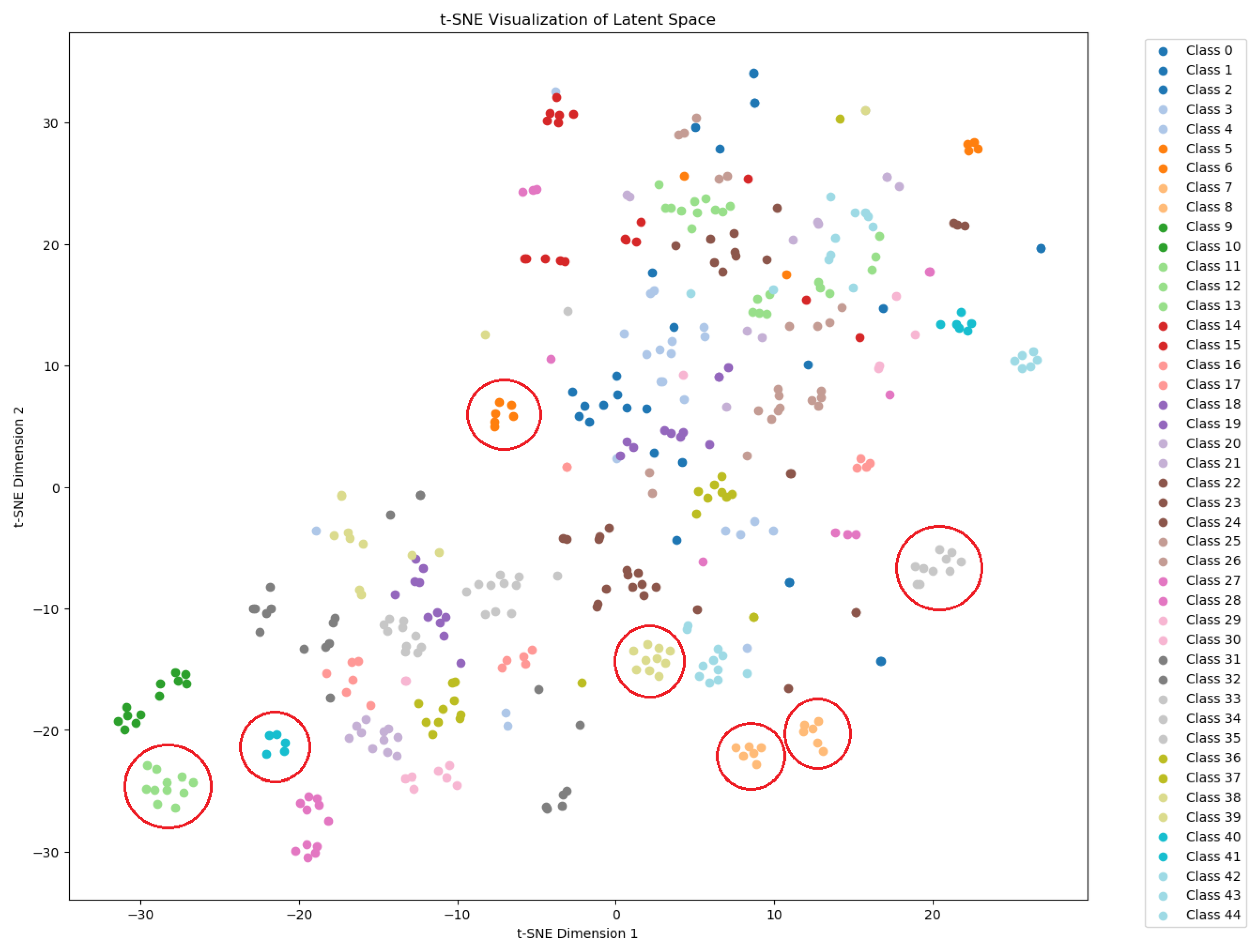
With a larger dataset, and especially for frames from recordings with poorer lighting conditions, the t-SNE visualization of features for dairy products clearly shows that distinct clusters are primarily formed by classes the model has already encountered during the training phase
Figure 8. If the model has seen a sufficient variety of different variants of a given brand, it can recognize a different variant of that product during the testing phase. The problem with identifying a product arises if the model has not previously encountered a similar shape or color scheme.
5. Conclusion
This study has successfully implemented a Variational Prototyping Encoder (VPE) tailored to the problem of recognizing retail shelf items from a limited dataset based on product graphics prototypes, achieving satisfactory accuracy. The strategic addition of prototypes to each training set notably improved the recognition rate of unseen classes, indicating a substantial improvement in the algorithm’s ability to identify new classes without prior exposure. Experiments also demonstrated the clear superiority of the cosine distance measure over the Euclidean one for this problem. Further comparisons showed that appropriately chosen and applied image sizes and augmentation techniques affect the algorithm’s performance. No significant differences were observed among the tested loss functions, but all proved effective in optimizing the model’s performance, confirming their usefulness for complex problems involving variational autoencoders. Uniform testing conditions for prototypes, such as consistent backgrounds and the selection of suitable prototypes, contributed to creating a cohesive assessment environment that yielded satisfactory effects.
The results highlighted variability in recognizability indicators across different product categories. The model excelled at recognizing various products of the same brand with similar packaging and labeling if it had encountered the class during the training phase. The model’s ability to generalize from training data was underscored by its performance on previously unseen variants of products from brands known from the training phase, demonstrating robustness in product recognition despite varying lighting conditions and presentations. Future work must continue to recognize products with shapes or colors that are not represented in the training set.
Further development possibilities include the application of diffusion models to the studied problem. Diffusion models, also known as diffusion probabilistic models or score-based generative models, are a class of latent variable generative models [
31]. Recent research increasingly supports the superiority of diffusion models compared to variational autoencoders. It is potentially possible to achieve more accurate and robust results by leveraging these advanced models. Such an improvement would pave the way for innovative solutions and a deeper understanding of the given problem.
Author Contributions
Conceptualization, G.S.; methodology, A.K.; software, A.K.; validation, G.S.; formal analysis, G.S.; investigation, A.K.; resources, G.S.; data curation, G.S.; writing—original draft preparation, A.K.; writing—review and editing, G.S.; visualization, A.K.; supervision, G.S.; project administration, G.S.; funding acquisition, G.S. All authors have read and agreed to the published version of the manuscript.
Funding
This research was co-founded by the National Center for Research and Development under Subtask 1.1.1 of the Smart Growth Operational Program 2014-2020, co-financed from public funds of the Regional Development Fund No. 2014/2020 under grant no. POIR.01.01.01-00-2326/20-00.
References
- Merler, M.; Galleguillos, C.; Belongie, S. Recognizing Groceries in situ Using in vitro Training Data. In Proceedings of the 2007 IEEE Conference on Computer Vision and Pattern Recognition; 2007; pp. 1–8. [Google Scholar] [CrossRef]
- Marder, M.; Harary, S.; Ribak, A.; Tzur, Y.; Alpert, S.; Tzadok, A. Using image analytics to monitor retail store shelves. IBM Journal of Research and Development 2015, 59, 3:1–3:11. [Google Scholar] [CrossRef]
- Kurzejamski, G.; Zawistowski, J.; Sarwas, G. A framework for robust object multi-detection with a vote aggregation and a cascade filtering. In Proceedings of the WSCG ’2015: short communications proceedings: The 23rd International Conference in Central Europe on Computer Graphics, 2015., Visualization and Computer Vision 2015 in co-operation with EUROGRAPHICS: University of West Bohemia. [Google Scholar]
- Kurzejamski, G.; Zawistowski, J.; Sarwas, G. Robust Method of Vote Aggregation and Proposition Verification for Invariant Local Features. In Proceedings of the Proceedings of the 10th International Conference on Computer Vision Theory and Applications - Volume 2: VISAPP, (VISIGRAPP 2015). INSTICC,SciTePress, 2015, pp.252–259. [CrossRef]
- George, M.; Mircic, D.; Sörös, G.; Floerkemeier, C.; Mattern, F. Fine-Grained Product Class Recognition for Assisted Shopping. In Proceedings of the 2015 IEEE International Conference on Computer Vision Workshop (ICCVW); 2015; pp. 546–554. [Google Scholar] [CrossRef]
- Melek, C.G.; Sonmez, E.B.; Albayrak, S. A survey of product recognition in shelf images. In Proceedings of the 2017 International Conference on Computer Science and Engineering (UBMK); 2017; pp. 145–150. [Google Scholar] [CrossRef]
- Tonioni, A.; Serra, E.; Di Stefano, L. A deep learning pipeline for product recognition on store shelves. In Proceedings of the 2018 IEEE International Conference on Image Processing, Applications and Systems (IPAS); 2018; pp. 25–31. [Google Scholar] [CrossRef]
- Geng, W.; Han, F.; Lin, J.; Zhu, L.; Bai, J.; Wang, S.; He, L.; Xiao, Q.; Lai, Z. Fine-Grained Grocery Product Recognition by One-Shot Learning. In Proceedings of the Proceedings of the 26th ACM International Conference on Multimedia, New York, NY, USA, 2018;MM’18; pp. 1706–1714. [CrossRef]
- Sun, H.; Hanata, K.; Sato, H.; Tsuchitani, I.; Akashi, T. Segmentation based Non-learning Product Detection for Product Recognition on Store Shelves. In Proceedings of the 2019 Nicograph International (NicoInt); 2019; pp. 9–16. [Google Scholar] [CrossRef]
- Leo, M.; Carcagnì, P.; Distante, C. A Systematic Investigation on end-to-end Deep Recognition of Grocery Products in the Wild. In Proceedings of the 2020 25th International Conference on Pattern Recognition (ICPR); 2021; pp. 7234–7241. [Google Scholar] [CrossRef]
- Chen, S.; Liu, D.; Pu, Y.; Zhong, Y. Advances in deep learning-based image recognition of product packaging. Image and Vision Computing 2022, 128, 104571. [Google Scholar] [CrossRef]
- Selvam, P.; Faheem, M.; Dakshinamurthi, V.; Nevgi, A.; Bhuvaneswari, R.; Deepak, K.; Abraham Sundar, J. Batch Normalization Free Rigorous Feature Flow Neural Network for Grocery Product Recognition. IEEE Access 2024, 12, 68364–68381. [Google Scholar] [CrossRef]
- Goldman, E.; Herzig, R.; Eisenschtat, A.; Goldberger, J.; Hassner, T. Precise Detection in Densely Packed Scenes. In Proceedings of the 2019 IEEE/CVF Conference on Computer Vision and Pattern Recognition (CVPR); 2019; pp. 5222–5231. [Google Scholar] [CrossRef]
- Melek, C.G.; Battini Sönmez, E.; Varlı, S. Datasets and methods of product recognition on grocery shelf images using computer vision and machine learning approaches: An exhaustive literature review. Engineering Applications of Artificial Intelligence 2024, 133, 108452. [Google Scholar] [CrossRef]
- Kim, J.; Oh, T.H.; Lee, S.; Pan, F.; Kweon, I.S. Variational Prototyping-Encoder: One-Shot Learning With Prototypical Images. In Proceedings of the 2019 IEEE/CVF Conference on Computer Vision and Pattern Recognition (CVPR); 2019; pp. 9454–9462. [Google Scholar] [CrossRef]
- Fe-Fei, L. ; Fergus. In ; Perona. A Bayesian approach to unsupervised one-shot learning of object categories. In Proceedings of the Proceedings Ninth IEEE International Conference on Computer Vision; 2003; pp. 1134–1141. [Google Scholar] [CrossRef]
- Lake, B.M.; Salakhutdinov, R.; Tenenbaum, J.B. Human-level concept learning through probabilistic program induction. Science 2015, 350, 1332–1338. [Google Scholar] [CrossRef] [PubMed]
- Vinyals, O.; Blundell, C.; Lillicrap, T.; kavukcuoglu, k.; Wierstra, D. Matching Networks for One Shot Learning. In Proceedings of the Advances in Neural Information Processing Systems; Lee, D.; Sugiyama, M.; Luxburg, U.; Guyon, I.; Garnett, R., Eds. Curran Associates, Inc., Vol. 29. 2016. [Google Scholar]
- Sung, F.; Yang, Y.; Zhang, L.; Xiang, T.; Torr, P.H.; Hospedales, T.M. Learning to Compare: Relation Network for Few-Shot Learning. In Proceedings of the 2018 IEEE/CVF Conference on Computer Vision and Pattern Recognition; 2018; pp. 1199–1208. [Google Scholar] [CrossRef]
- Zhenguo, L.; Fengwei, Z.; Fei, C.; Hang, L. Meta-SGD: Learning to Learn Quickly for Few Shot Learning. ArXiv 2017, abs/1707.09835. [Google Scholar]
- Finn, C.; Abbeel, P.; Levine, S. Model-agnostic meta-learning for fast adaptation of deep networks. In Proceedings of the Proceedings of the 34th International Conference on Machine Learning - Volume 70.; pp. 2017101126–1135.
- Chen, T.; Xie, G.S.; Yao, Y.; Wang, Q.; Shen, F.; Tang, Z.; Zhang, J. Semantically Meaningful Class Prototype Learning for One-Shot Image Segmentation. IEEE Transactions on Multimedia 2022, 24, 968–980. [Google Scholar] [CrossRef]
- Snell, J.; Swersky, K.; Zemel, R. Prototypical Networks for Few-shot Learning. In Proceedings of the Advances in Neural Information Processing Systems; Guyon, I.; Luxburg, U.V.; Bengio, S.; Wallach, H.; Fergus, R.; Vishwanathan, S.; Garnett, R., Eds. Curran Associates, Inc., Vol. 30. 2017. [Google Scholar]
- Wang, C.; Huang, C.; Zhu, X.; Zhao, L. One-Shot Retail Product Identification Based on Improved Siamese Neural Networks. Circuits, Systems, and Signal Processing 2022, 41, 1–15. [Google Scholar] [CrossRef]
- Kingma, D.P.; Welling, M. Auto-Encoding Variational Bayes. In Proceedings of the 2nd International Conference on Learning Representations, ICLR 2014, Banff, AB, Canada, 2014, Conference Track Proceedings, 2014, [http://arxiv.org/abs/1312.6114v10]., April 14-16.
- Kang, J.S.; Ahn, S.C. Variational Multi-Prototype Encoder for Object Recognition Using Multiple Prototype Images. IEEE Access 2022, 10, 19586–19598. [Google Scholar] [CrossRef]
- Liu, Y.; Shi, D. SS-VPE: Semi-Supervised Variational Prototyping Encoder With Student’s-t Mixture Model. IEEE Transactions on Instrumentation and Measurement 2023, 72, 1–9. [Google Scholar] [CrossRef]
- Xiao, C.; Madapana, N.; Wachs, J. One-Shot Image Recognition Using Prototypical Encoders with Reduced Hubness. In Proceedings of the 2021 IEEE Winter Conference on Applications of Computer Vision (WACV); 2021; pp. 2251–2260. [Google Scholar] [CrossRef]
- Panchal, S. Implementation and Comparative Quantitative Assessment of Different Multispectral Image Pansharpening Approaches. Signal & Image processing:An International Journal 2015, 6, 35. [Google Scholar] [CrossRef]
- Kirillov, A.; Mintun, E.; Ravi, N.; Mao, H.; Rolland, C.; Gustafson, L.; Xiao, T.; Whitehead, S.; Berg, A.C.; Lo, W.Y.; et al. Segment Anything. In Proceedings of the Proceedings of the IEEE/CVF International Conference on Computer Vision (ICCV), October 2023; pp. 4015–4026.
- Hu, R.; Hu, W.; Li, J. Saliency Driven Nonlinear Diffusion Filtering for Object Recognition. In Proceedings of the 2013 2nd IAPR Asian Conference on Pattern Recognition; 2013; pp. 381–385. [Google Scholar] [CrossRef]
Short Biography of Authors
 |
Aleksandra Kowalczyk received her B.S. degree in Computer Science in 2023 and M.Sc. in Computer Science in 2024, both from the Faculty of Electrical Engineering at the Warsaw University of Technology. She works professionally as a Data Engineer. Her research interests include machine learning, deep learning, and computer vision. |
 |
Grzegorze Sarwas received his M.Sc. degree in Electrical Engineering, majoring in Control and Computer Engineering, from Warsaw University of Technology in 2007 and his Ph.D. in Automation and Robotics in 2013. He has been actively engaged in R&D projects in computer vision and data analysis with several companies. Since 2016, he has been an assistant professor at the Warsaw University of Technology, focusing his research on image processing, computer vision, and data modeling. |
|
Disclaimer/Publisher’s Note: The statements, opinions and data contained in all publications are solely those of the individual author(s) and contributor(s) and not of MDPI and/or the editor(s). MDPI and/or the editor(s) disclaim responsibility for any injury to people or property resulting from any ideas, methods, instructions or products referred to in the content. |
© 2024 by the authors. Licensee MDPI, Basel, Switzerland. This article is an open access article distributed under the terms and conditions of the Creative Commons Attribution (CC BY) license (http://creativecommons.org/licenses/by/4.0/).
