Submitted:
11 July 2024
Posted:
12 July 2024
You are already at the latest version
Abstract
Keywords:
1. Introduction
2. Upper-Air Physics
2.1. Radiation
2.2. Convection
2.3. Turbulence
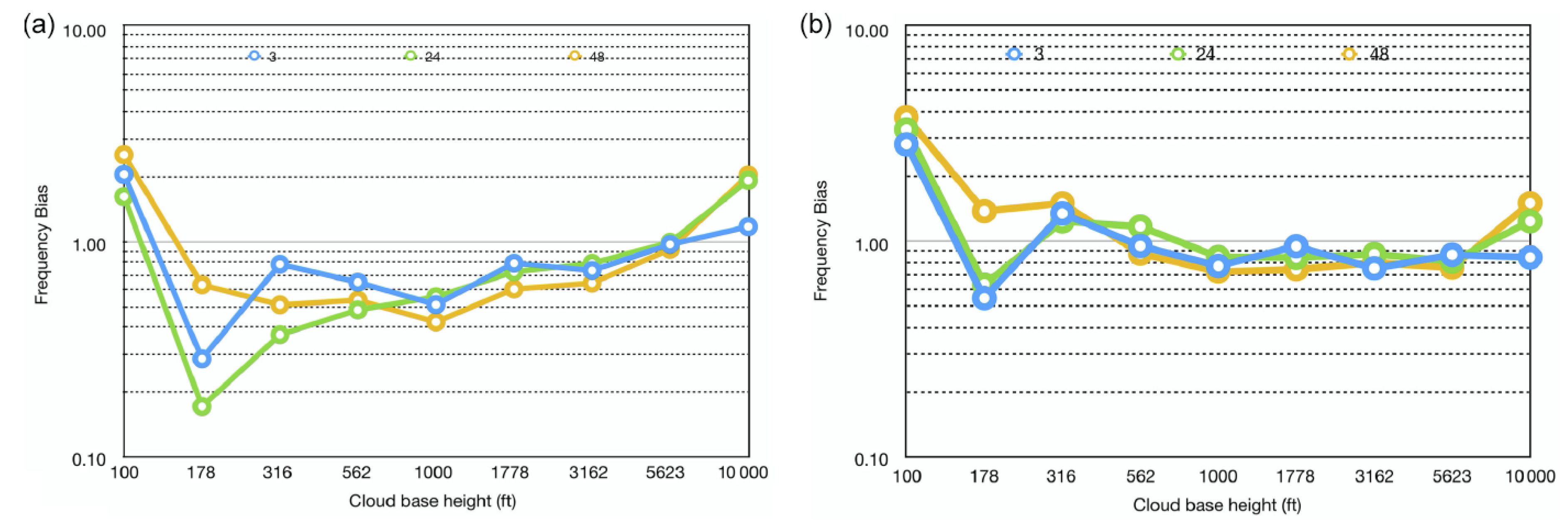
2.4. Statistical Cloud Scheme
- A proper derivation of the thermodynamic coefficients.
- The inclusion of the covariance term of temperature and humidity.
- Using a dissipation length scale that is consistent with the one in the turbulence scheme.
- The description of the dissipation of the variances is more consistent with literature.
- An erroneous factor 2 for the convective contribution to the variance is removed.
2.5. Cloud Microphysics
2.5.1. Cloud Droplet Number Concentration
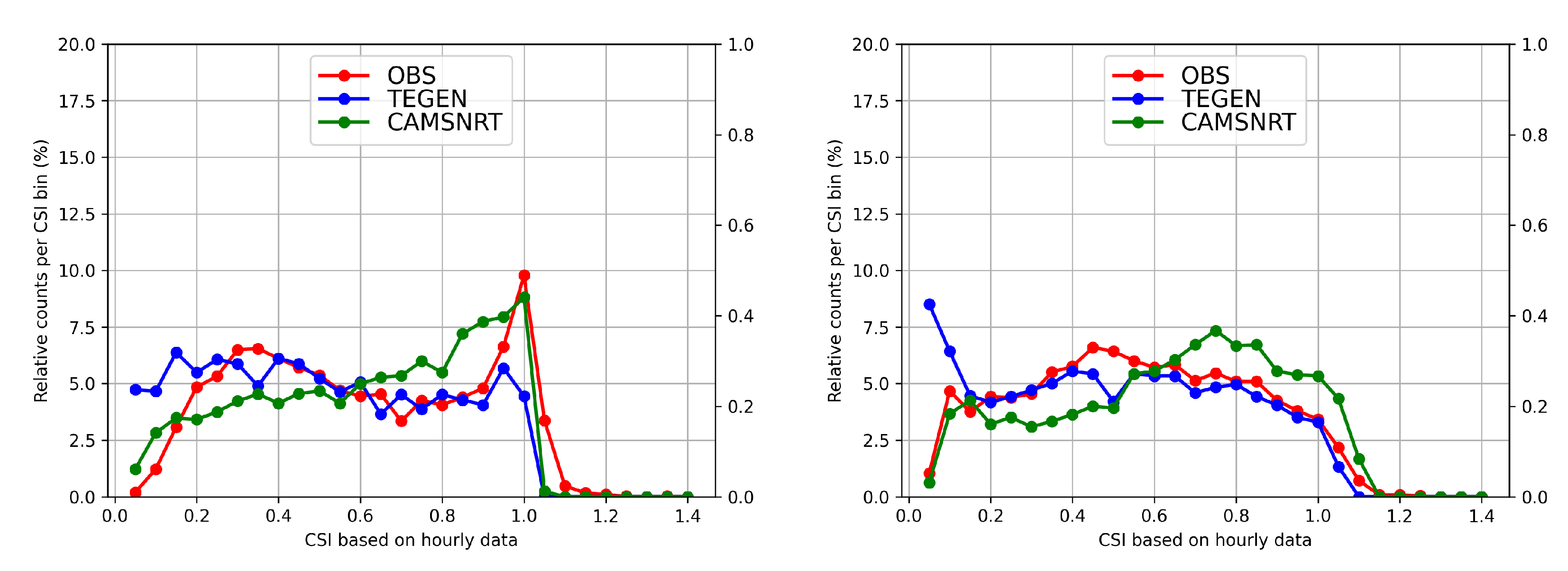
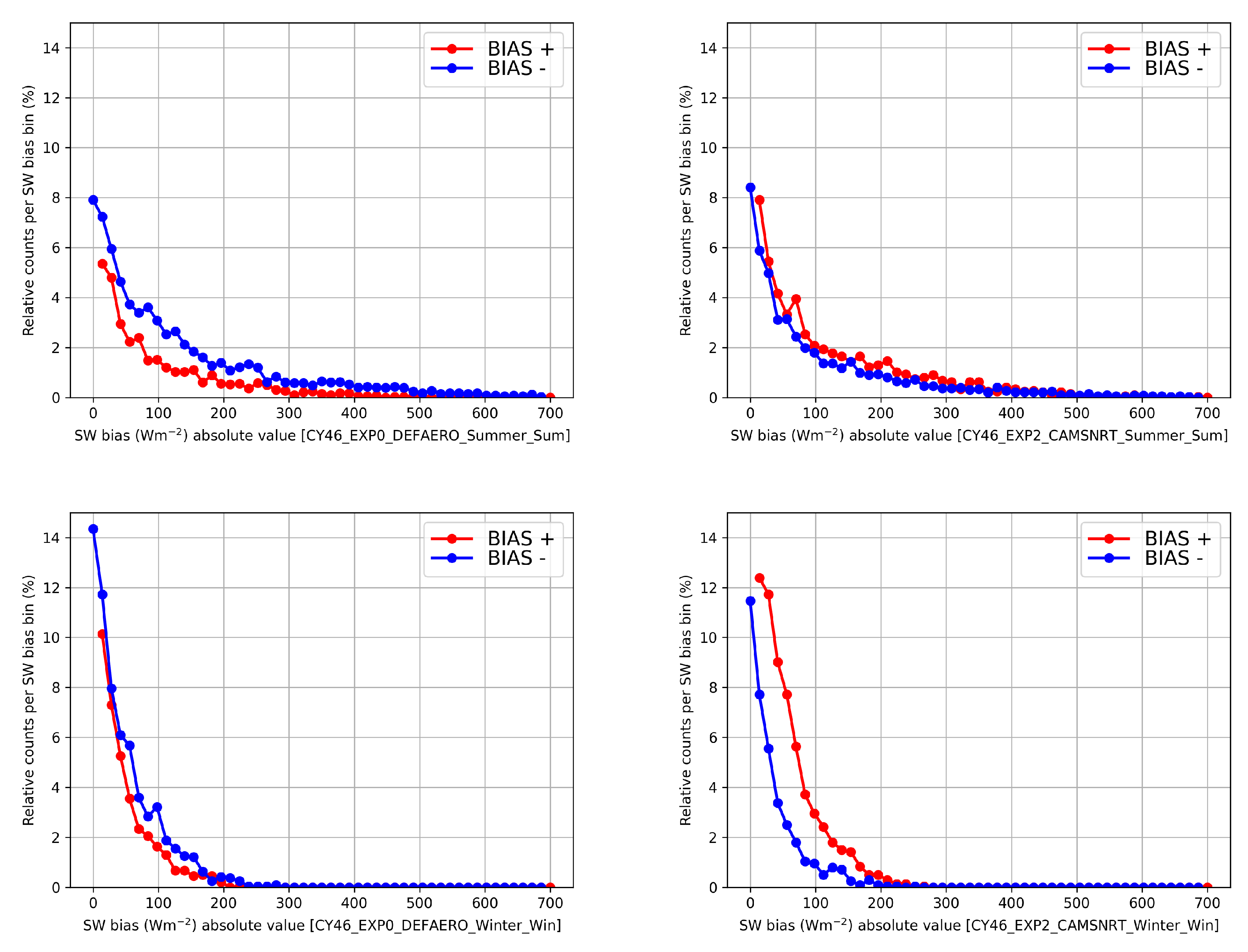
2.5.2. Use of CAMS NRT Aerosols in ICE3
2.5.3. OCND2
- The separation between liquid water processes and ice water processes was improved. This means that the statistical cloud scheme (See Section 2.4) only deals with cloud liquid water, including cases when temperatures are below freezing. Thus, all ice processes are taken care of by the OCND2 version of the ICE3 scheme.
- Evaporation/deposition of cloud ice water is a conversion between ice and vapour and not between ice and liquid.
- The deposition rate of the ice water species was reduced.
- The cloud cover, from the point of view of users of the forecast (the public), was modified to account for the lower optical thickness of ice clouds compared to water clouds.
- The ice number concentration was reduced between temperatures of C and C. The main purpose of this is to slow down the conversion from cloud liquid water to ice, snow or graupel.
- To support the production of supercooled rain, threshold values were introduced for converting supercooled rain into graupel or snow
- Avoid calculations of saturation pressure when the saturation pressure is near or above atmospheric pressure. This is done just for technical reasons, and affects calculations in the Stratosphere only.
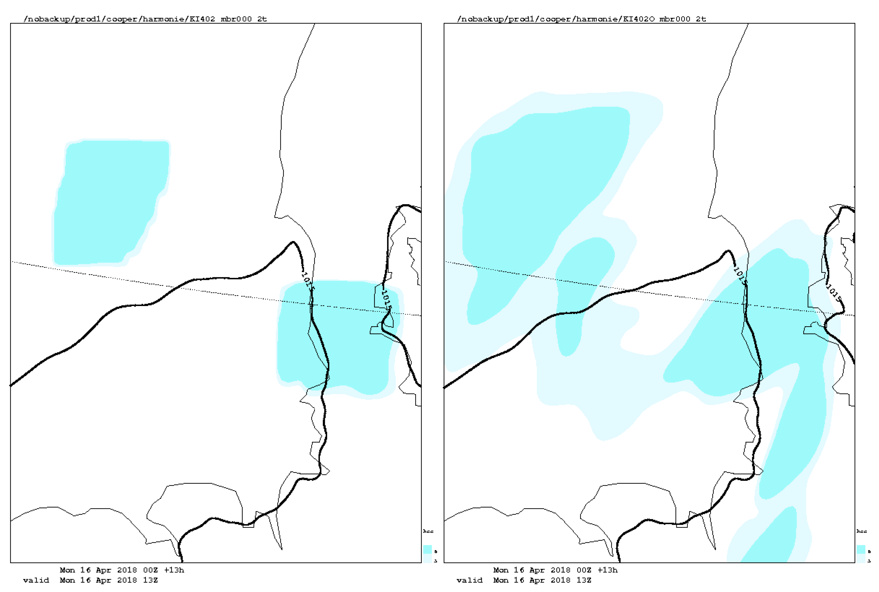
- In order to save computing time, the ICE3 scheme should be active only when any non-vapour water species are present above a low threshold, or when the air temperature is below freezing. Unfortunately, this did not always happen when the second criteria was satisfied. This occasionally led to spurious square-like ice-clouds where areas with sufficient water species are surrounded by areas with too little cloud ice water, as shown in Figure 11. A fix has now been implemented.
2.5.4. ICE-T
- Stricter conditions for ice nucleation.
- Less efficient collision-collection of liquid water by solid hydrometeors.
- A variable rain intercept parameter, which allows for smaller droplets when condensation and coalescence are the primary sources.

3. Surface Physics
3.1. Physiography
3.2. The Urban and Nature Tiles
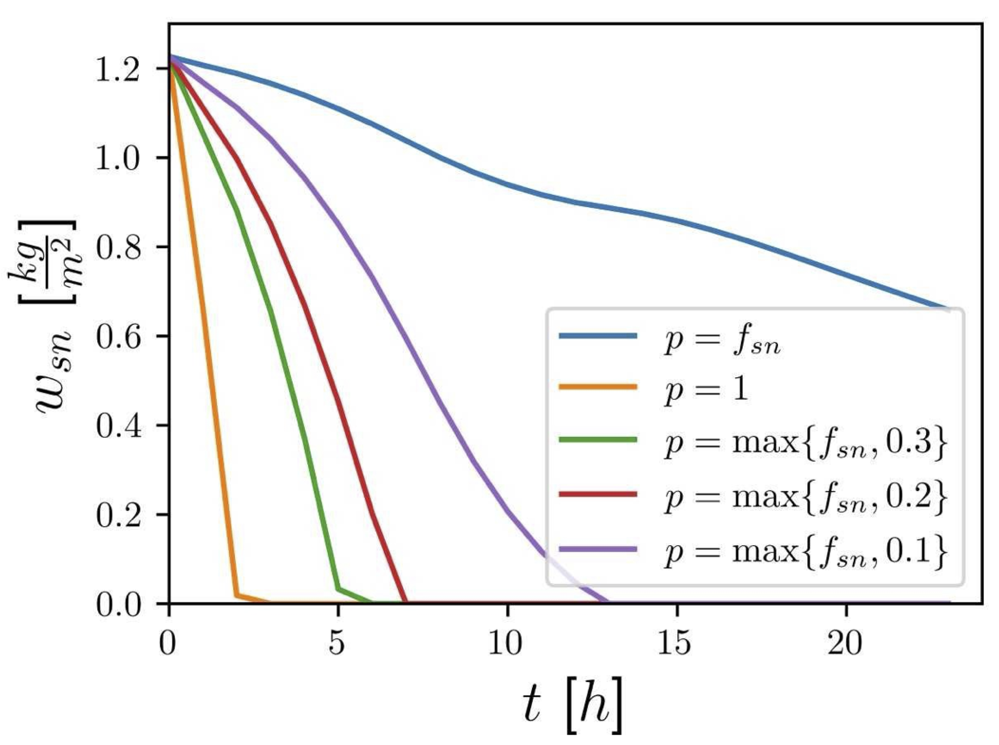
3.3. Snow Melt Adjustment
3.4. Stable Boundary Layer
3.5. Orographic Enhancement of Momentum Fluxes
3.6. The Sea Tile
3.7. The Inland water Tile
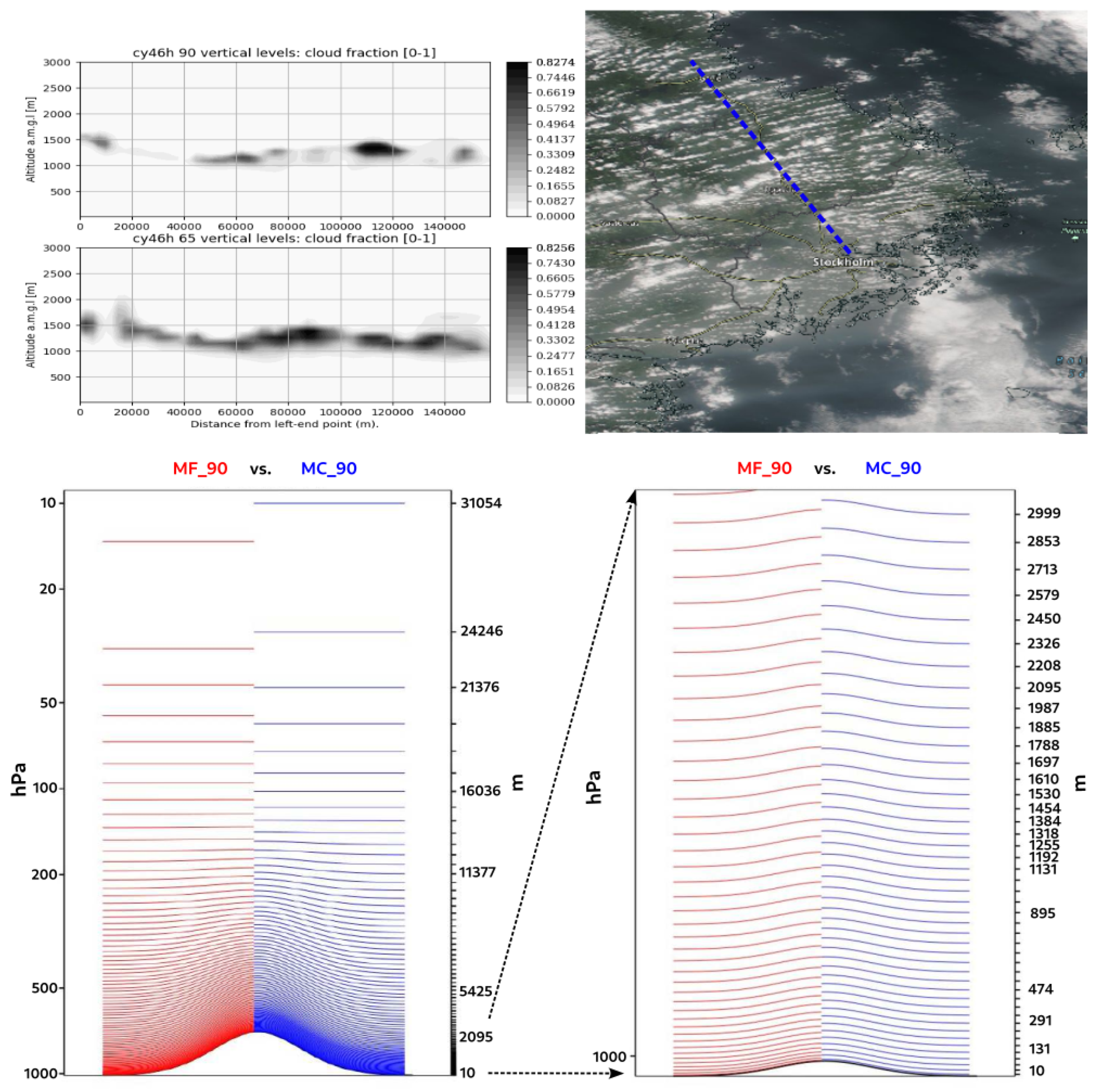
4. Dynamics and Model Configuration
5. Upcoming Developments in HARMONIE-AROME
5.1. Radiation
5.2. Scale Aware Shallow Convection
5.3. Cloud Microphysics
5.4. Surface
5.5. Dynamics and Model Configuration
Author Contributions
Acknowledgments
Conflicts of Interest
| 1 | Note that the other coefficients were not investigated in this study. |
| 2 | MetCoOp started in 2010 with MET Norway and the Swedish Meteorological and Hydrological Institute collaborating on the production of operational weather forecasts. The Finnish Meteorological Institute joined in 2017, with Estonia, Latvia and Lithuania following in 2022. |
| 3 | In 2021 the National Meteorological Services of Ireland, Denmark, Iceland and the Netherlands joined forces operationally, a grouping now known as United Weather Centers - West (UWC-West). |
| 4 | UWC-West already is using the option operationally, while MetCoOP is using in pre-operational mode. |
References
- Malardel, S. MUSC : (Modèle Unifié, Simple Colonne) for Arpege-Aladin-Arome-Alaro-Hirlam-(IFS) (CY31T1 version). Technical report, Météo France, 2004. (last access: 24 May 2024).
- Mlawer, E.J.; Taubman, S.J.; Brown, P.D.; Iacono, M.J.; Clough, S.A. Radiative transfer for inhomogeneous atmospheres: RRTM, a validated correlated-k model for the longwave. Journal of Geophysical Research: Atmospheres 1997, 102, 16663–16682, [https://agupubs.onlinelibrary.wiley.com/doi/pdf/10.1029/97JD00237]. [CrossRef]
- ECMWF. Operational implementation 12 May 2015. Part IV: Physical processes. European Centre for Medium-Range Weather Forecasts IFS Doc. Cy41r1. Technical report, ECMWF, 2015.
- Mascart, P.J.; Bougeault, P. The Meso-NH atmospheric simulation system: Scientific documentation. Part III: Physics. Technical report, Météo-France, 2011.
- Mašek, J.; Geleyn, J.F.; Brožková, R.; Giot, O.; Achom, H.O.; Kuma, P. Single interval shortwave radiation scheme with parameterized optical saturation and spectral overlaps. Quarterly Journal of the Royal Meteorological Society 2016, 142, 304–326. [CrossRef]
- Geleyn, J.F.; Mašek, J.; Brožková, R.; Kuma, P.; Degrauwe, D.; Hello, G.; Pristov, N. Single interval longwave radiation scheme based on the net exchanged rate decomposition with bracketing. Quarterly Journal of the Royal Meteorological Society 2017, 143, 1313–1335. [CrossRef]
- Kangas, M.; Rontu, L.; Fortelius, C.; Aurela, M.; Poikonen, A. Weather model verification using Sodankylä mast measurements. Geoscientific Instrumentation, Methods and Data Systems 2016, 5, 75–84. [CrossRef]
- Rontu, L.; Lindfors, A.V. Comparison of radiation parametrizations within the HARMONIE–AROME NWP model. Advances in Science and Research 2018, 15, 81–90. [CrossRef]
- Tegen, I.; Hollrig, P.; Chin, M.; Fung, I.; Jacob, D.; Penner, J. Contribution of different aerosol species to the global aerosol extinction optical thickness: Estimates from model results. Journal of Geophysical Research: Atmospheres 1997, 102, 23895–23915, [https://agupubs.onlinelibrary.wiley.com/doi/pdf/10.1029/97JD01864]. [CrossRef]
- Martín Pérez, D.; Gleeson, E.; Maalampi, P.; Rontu, L. Use of CAMS near real-time aerosols in the HARMONIE-AROME NWP model. Meteorology 2024. Under review.
- Bozzo, A.; Benedetti, A.; Flemming, J.; Kipling, Z.; Rémy, S. An aerosol climatology for global models based on the tropospheric aerosol scheme in the Integrated Forecasting System of ECMWF. Geoscientific Model Development 2020, 13, 1007–1034. [CrossRef]
- Kettler, T. Fog Forecasting in HARMONIE - a case study to current issues with the overestimation of fog in HARMONIE, 2020. Utrecht University, Master’s thesis.
- Smith, E.A.; Shi, L. Surface Forcing of the Infrared Cooling Profile over the Tibetan Plateau. Part I: Influence of Relative Longwave Radiative Heating at High Altitude. Journal of the Atmospheric Sciences 1992, 49, 805–822.
- Elsasser, W.M. Heat Transfer by Infrared Radiation in the Atmosphere; Harvard University, Milton, MA, USA, 1942.
- de Rooy, W.C.; Siebesma, A.; Baas, P.; Lenderink, G.; de Roode, S.; de Vries, H.; van Meijgaard, E.; Meirink, J.F.; Tijm, S.; van ’t Veen, B. Model development in practice: a comprehensive update to the boundary layer schemes in HARMONIE-AROME cycle 40. Geosci. Model Dev. 2022, 15, 1513–1543. [CrossRef]
- Kähnert, M.; Sodemann, H.; de Rooy, W.C.; Valkonen, T.M. On the Utility of Individual Tendency Output: Revealing Interactions between Parameterized Processes during a Marine Cold Air Outbreak. Weather and Forecasting 2021, 36, 1985 – 2000. [CrossRef]
- Neggers, R.; Kohler, M.; Beljaars, A. A dual mass flux framework for boundary layer convection. Part I: Transport. J. Atmos. Sci. 2009, 66, 1464–1487.
- de Roode, S.; Duynkerke, P.; Siebesma, A. Analogies Between Mass-Flux and Reynolds-Averaged Equations. J. Atmos. Sci. 2000, 57, 1585–1598. [CrossRef]
- Lenderink, G.; Holtslag, A. An Updated Length-Scale Formulation for Turbulent Mixing in Clear and Cloudy Boundary Layers. QJRMS 2004, 130, 3405–3427. [CrossRef]
- Cuxart, J.; Bougeault, P.; Redelsperger, J.L. A Turbulence Scheme Allowing for Mesoscale and Large-Eddy Simulations. Quart. J. Roy. Meteor. Soc. 2000, 126, 1–30. [CrossRef]
- de Rooy, W.C. The Fog Above Sea Problem: Part 1 Analysis. ALADIN-HIRLAM Newsletter 2014, 2, 9–16. (last access: 11 January 2022).
- de Rooy, W.C.; de Vries, H.; et al.. Harmonie Verification and Evaluation. Technical Report 70, Hirlam, 2017. (last access: 11 January 2022).
- Baas, P.; de Roode, S.R.; Lenderink, G. The scaling behaviour of a turbulent kinetic energy closure model for stably stratified conditions. Boundary-layer meteorology 2008, 127, 17–36.
- Baas, P.; Van De Wiel, B.; Van der Linden, S.; Bosveld, F. From near-neutral to strongly stratified: Adequately modelling the clear-sky nocturnal boundary layer at Cabauw. Boundary-Layer Meteorology 2018, 166, 217–238.
- Van Stratum, B.; Theeuwes, N.; Barkmeijer, J.; van Ulft, B.; Wijnant, I. A One-Year-Long Evaluation of a Wind-Farm Parameterization in HARMONIE-AROME. Journal of Advances in Modeling Earth Systems 2022, 14, e2021MS002947.
- Sommeria, G.; Deardorff, J. Subgrid-Scale Condensation in Models of Non-Precipitating Clouds. J. Atmos. Sci. 1977, 34, 344–355. [CrossRef]
- Brown, A.R.; Cederwall, R.T.; Chlond, A.; Duynkerke, P.G.; Golaz, J.C.; Khairoutdinov, M.; Lewellen, D.C.; Lock, A.P.; MacVean, M.K.; Moeng, C.H.; Neggers, R.A.J.; Siebesma, A.P.; Stevens, B. Large-eddy simulation of the diurnal cycle of shallow cumulus convection over land. Quarterly Journal of the Royal Meteorological Society 2002, 128, 1075–1093, [https://rmets.onlinelibrary.wiley.com/doi/pdf/10.1256/003590002320373210]. [CrossRef]
- Lascaux, F.; Richard, E.; Pinty, J.P. Numerical simulations of three different MAP IOPs and the associated microphysical processes. Quarterly Journal of the Royal Meteorological Society 2006, 132, 1907–1926, [https://rmets.onlinelibrary.wiley.com/doi/pdf/10.1256/qj.05.197]. [CrossRef]
- Pinty, J.P.; Jabouille, P. A Mixed-Phased Cloud Parameterization for Use in a Mesoscale Non-Hydrostatic Model: Simulations of a Squall Line and of Orographic Precipitation. Conference on Cloud Physics; , 1998; pp. 217–220.
- Bénard, P.; Vivoda, J.; Mašek, J.; Smolíková, P.; Yessad, K.; Smith, C.; Brožková, R.; Geleyn, J.F. Dynamical kernel of the Aladin–NH spectral limited-area model: Revised formulation and sensitivity experiments. Quarterly Journal of the Royal Meteorological Society 2010, 136, 155–169, [https://rmets.onlinelibrary.wiley.com/doi/pdf/10.1002/qj.522]. [CrossRef]
- Bouteloup, Y.; Seity, Y.; Bazile, E. Description of the sedimentation scheme used operationally in all M et eo-France NWP models. Tellus A: Dynamic Meteorology and Oceanography 2011, 63, 300–311.
- Contreras Osorio, S.; Martín Pérez, D.; Ivarsson, K.I.; Nielsen, K.P.; de Rooy, W.C.; Gleeson, E.; McAufield, E. Impact of the Microphysics in HARMONIE-AROME on Fog. Atmosphere 2022, 13, 2127. Number: 12 Publisher: Multidisciplinary Digital Publishing Institute, . [CrossRef]
- Meinander, O.; Kouznetsov, R.; Uppstu, A.; Sofiev, M.; Kaakinen, A.; Salminen, J.; Rontu, L.; Welti, A.; Francis, D.; Piedehierro, A.A.; Heikkilä, P.; Heikkinen, E.; Laaksonen, A. African dust transport and deposition modelling verified through a citizen science campaign in Finland. Scientific Reports 2023, 13, 21379. [CrossRef]
- Müller, M.; Homleid, M.; Ivarsson, K.I.; Morten A. . Køltzow.; Lindskog, M.; Midtbø, K.H.; Andrae, U.; Aspelien, T.; Berggren, L.; Bjørge, D.; Dahlgren, P.; Kristiansen, J.; Randriamampianina, R.; Ridal, M.; Vignes, O. AROME-MetCoOp: A Nordic Convective-Scale Operational Weather Prediction Model. Weather and Forecasting 2017, 32, 609 – 627. [CrossRef]
- Engdahl, B.J.K.; Nygaard, B.E.K.; Losnedal, V.; Thompson, G.; Bengtsson, L. Effects of the ICE-T microphysics scheme in HARMONIE-AROME on estimated ice loads on transmission lines. Cold Reg. Sci. Technol. 2020, 179, 103139.
- Thompson, G.; Field, P.R.; Rasmussen, R.M.; Hall, W.D. Explicit Forecasts of Winter Precipitation Using an Improved Bulk Microphysics Scheme. Part II: Implementation of a New Snow Parameterization. Mon. Weather Rev. 2008, 136, 5095–5115.
- Engdahl, B.J.K.; Thompson, G.; Bengtsson, L. Improving the representation of supercooled liquid water in the HARMONIE-AROME weather forecast model. Tellus Ser. A Dyn. Meteorol. Oceanogr. 2020, 72, 1–18.
- Engdahl, B.J.K.; Carlsen, T.; Køltzow, M.; Storelvmo, T. The Ability of the ICE-T Microphysics Scheme in HARMONIE-AROME to Predict Aircraft Icing. Weather and Forecasting 2022, 37, 205 – 217. [CrossRef]
- Le Moigne, P. Surfex scientific documentation. Météo-France 2018.
- Faroux, S.; Kaptué Tchuenté, A.T.; Roujean, J.L.; Masson, V.; Martin, E.; Le Moigne, P. ECOCLIMAP-II/Europe: A twofold database of ecosystems and surface parameters at 1 km resolution based on satellite information for use in land surface, meteorological and climate models. Geosci. Model Dev. 2013, 6, 563–582. [CrossRef]
- Choulga, M.; Kourzeneva, E.; Zakharova, E.; Doganovsky, A. Estimation of the mean depth of boreal lakes for use in numerical weather prediction and climate modelling. Tellus 2014, 66A. [CrossRef]
- Kourzeneva, E.; Martin, E.; Batrak, Y.; Le Moigne, P. Climate data for parameterisation of lakes in Numerical Weather Prediction models. Tellus 2012, 64A. [CrossRef]
- Masson, V. A physically-based scheme for the urban energy budget in atmospheric models. Boundary-Layer Meteorology 2000, 94, 357–397. [CrossRef]
- Boone, A.; Calvet, J.C.; Noilhan, J. Inclusion of a third soil layer in a land surface scheme using the force–restore method. J. Appl. Meteor. 1999, 38, 1611–1630.
- Douville, H.; Royer, J.F.; Mahfouf, J.F. A new snow parameterization for theMétéo-France climate model. Part I: Validation in stand-alone experiments. Climate Dynamics 1995, 12, 21–35. [CrossRef]
- Atlaskin, E.; Vihma, T. Evaluation of NWP results for wintertime nocturnal boundary-layer temperatures over Europe and Finland. Quart. J. Roy. Meteor. Soc. 2012, 138. [CrossRef]
- Kähnert, M.; Sodemann, H.; Remes, T.M.; Fortelius, C.; Bazile, E.; Esau, I. Spatial variability of nocturnal stability regimes in an operational weather prediction model. Boundary-Layer Meteorology 2023, 186, 373–397.
- Svensson, G.; Holtslag, A.A.M. Analysis of Model Results for the Turning of the Wind and Related Momentum Fluxes in the Stable Boundary Layer. Boundary-Layer Meteorology 2009, 132, 261–277. [CrossRef]
- Viterbo, P.; Beljaars, A.; Mahfouf, J.F.; Teixeira, J. The representation of soil moisture freezing and its impact on the stable boundary layer. Quart. J. Roy. Meteor. Soc. 1999, 125, 2401–2426. [CrossRef]
- Sandu, I.; Beljaars, A.; Bechtold, P.; Mauritsen, T.; Balsamo, G. Why is it so difficult to represent stably stratified conditions in numerical weather prediction (NWP) models? Journal of Advances in Modeling Earth Systems 2013, 5, 117–133. [CrossRef]
- Homleid, M. Improving model performance in stable situations by using a pragmatic shift in the drag calculations - XRISHIFT. ACCORD Newsletter 2 2022, pp. 96–108.
- Kähnert, M.; Sodemann, H.; Remes, T.M.; Homleid, M. On the crux of surface coupling during stable conditions - A model-tuning study. submitted to Weather and Forecasting 2024.
- Mason, P.J. On the parameterization of the orographic drag. Technical report, ECMWF, 1985. Proc. Seminar on Physical parametrization for Numerical Models of the Atmosphere.
- Georgelin, M.; Richard, E.; Petitdidier, M.; Druilhet, A. Impact of subgrid-scale orography parametrization on the simulation orographic flows. Mon. Wea. Rev 1994, 122, 1509–1522.
- Wood, N.; Brown, A.R.; Hewer, F.E. Parametrizing the effects of orography on the boundary layer: An alternative to effective roughness lengths. Quarterly Journal of the Royal Meteorological Society 2001, 127, 759–777. [CrossRef]
- Beljaars, A.C.M.; Brown, A.R.; Wood, N. A new parametrization of turbulent orographic form drag. Q. J. R. Meteor. Soc. 2004, 130, 1327–1347.
- Rontu, L. A study on parametrization of orography-related momentum fluxes in a synoptic-scale NWP model. Tellus A: Dynamic Meteorology and Oceanography 2006, 58, 69–81. [CrossRef]
- Calvo, J.; Campins, J.; María Díez, M.; Escribà, P.; Martín, D.; Gema Morales, G.; Sánchez-Arriola, J.; Viana, S. Evaluation of HARMONIE-AROME cycle 43h2.1 at AEMET. Newsletter 2022, pp. 166–172.
- Bougeault, P.; Lacarrere, P. Parameterisation of orography-induced turbulence in a meso-beta scale Model. Mon. Wea. Rev. 1989, 117, 1872–1890.
- Madec, G.; Bell, M.; Balker, A.; Bricaud, C.; Bruciaferry, D.; Castrillo, M.; Calvert, D.; Chanut, J.; Clementi, E.; Coward, A.; Epicoco, I.; Éthé, C.; Ganderton, J.; Harle, J.; Hutchinson, K.; Iovino, D.; Lea, D.; Lovato, T.; Martin, M.; Wilson, C. NEMO Ocean Engine Reference Manual. Scientific Notes of IPSL Climate Modelling Center 2023, 4.2.1. [CrossRef]
- Belušić, D.; de Vries, H.; Dobler, A.; Landgren, O.; Lind, P.; Lindstedt, D.; Pedersen, R.A.; Sánchez-Perrino, J.C.; Toivonen, E.; van Ulft, B.; Wang, F.; Andrae, U.; Batrak, Y.; Kjellström, E.; Lenderink, G.; Nikulin, G.; Pietikäinen, J.P.; Rodríguez-Camino, E.; Samuelsson, P.; van Meijgaard, E.; Wu, M. HCLIM38: a flexible regional climate model applicable for different climate zones from coarse to convection-permitting scales. Geoscientific Model Development 2020, 13, 1311–1333. [CrossRef]
- Belamari, S. Report on uncertainty estimates of an optimal bulk formulation for surface turbulent fluxes. Marine Environment and Security for the European Area–Integrated Project MERSEA IP Deliverable D4.1.2 2005, pp. 1–29.
- van den Brekel, S. Validating the surface flux ECUME and ECUME6 parameterizations used in the HARMONIE model, 2023. Master’s thesis, available at http://repository.tudelft.nl/.
- Batrak, Y.; Kourzeneva, E.; Homleid, M. Implementation of a simple thermodynamic sea ice scheme, SICE version 1.0-38h1, within the ALADIN–HIRLAM numerical weather prediction system version 38h1. Geoscientific Model Development 2018, 11, 3347–3368. [CrossRef]
- Batrak, Y.; Müller, M. On the warm bias in atmospheric reanalyses induced by the missing snow over Arctic sea-ice. Nature Communications 2019, 10, 4170. [CrossRef]
- Mironov, D.; Heise, E.; Kourzeneva, E.; Ritter, B.; Schneider, N.; Terzhevik, A. Implementation of the lake parameterisation scheme FLake into the numerical weather prediction model COSMO. Boreal Environmental Research 2010, 15, 218–230.
- Semmler, T.; Cheng, B.; Yang, Y.; Rontu, L. Snow and ice on Bear Lake (Alaska) - sensitivity experiments with two lake ice models. Tellus 2012, 64A. [CrossRef]
- Bubnová, R.; Hello, G.; Bénard, P.; Geleyn, J.F. Integration of the Fully Elastic Equations Cast in the Hydrostatic Pressure Terrain-Following Coordinate in the Framework of the ARPEGE/Aladin NWP System. Monthly Weather Review 1995, 123, 515 – 535. [CrossRef]
- Termonia, P.; Fischer, C.; Bazile, E.; Bouyssel, F.; Brožková, R.; Bénard, P.; Bochenek, B.; Degrauwe, D.; Derková, M.; El Khatib, R.; Hamdi, R.; Mašek, J.; Pottier, P.; Pristov, N.; Seity, Y.; Smolíková, P.; Španiel, O.; Tudor, M.; Wang, Y.; Wittmann, C.; Joly, A. The ALADIN System and its canonical model configurations AROME CY41T1 and ALARO CY40T1. Geoscientific Model Development 2018, 11, 257–281. [CrossRef]
- Seity, Y.; Brousseau, P.; Malardel, S.; Hello, G.; Bénard, P.; Bouttier, F.; Lac, C.; Masson, V. The AROME-France Convective-Scale Operational Model. Monthly Weather Review 2011, 139, 976 – 991. [CrossRef]
- Laprise, R. The Euler Equations of Motion with Hydrostatic Pressure as an Independent Variable. Monthly Weather Review 1992, 120, 197 – 207. [CrossRef]
- Simmons, A.J.; Burridge, D.M. An Energy and Angular-Momentum Conserving Vertical Finite-Difference Scheme and Hybrid Vertical Coordinates. Monthly Weather Review 1981, 109, 758 – 766. [CrossRef]
- Hortal, M. The development and testing of a new two-time-level semi-Lagrangian scheme (SETTLS) in the ECMWF forecast model. Quarterly Journal of the Royal Meteorological Society 2002, 128, 1671–1687, [https://rmets.onlinelibrary.wiley.com/doi/pdf/10.1002/qj.200212858314]. [CrossRef]
- Davies, H.C. A lateral boundary formulation for multi-level prediction models. Quarterly Journal of the Royal Meteorological Society 1976, 102, 405–418, [https://rmets.onlinelibrary.wiley.com/doi/pdf/10.1002/qj.49710243210]. [CrossRef]
- Váňa, F.; Bénard, P.; Geleyn, J.F.; Simon, A.; Seity, Y. Semi-Lagrangian advection scheme with controlled damping: An alternative to nonlinear horizontal diffusion in a numerical weather prediction model. Quarterly Journal of the Royal Meteorological Society 2008, 134, 523–537.
- Malardel, S.; Ricard, D. An alternative cell-averaged departure point reconstruction for pointwise semi-Lagrangian transport schemes. Quarterly Journal of the Royal Meteorological Society 2015, 141, 2114–2126, [https://rmets.onlinelibrary.wiley.com/doi/pdf/10.1002/qj.2509]. [CrossRef]
- Lang, S.T.K.; Dawson, A.; Diamantakis, M.; Dueben, P.; Hatfield, S.; Leutbecher, M.; Palmer, T.; Prates, F.; Roberts, C.D.; Sandu, I.; Wedi, N. More accuracy with less precision. Quarterly Journal of the Royal Meteorological Society 2021, 147, 4358–4370, [https://rmets.onlinelibrary.wiley.com/doi/pdf/10.1002/qj.4181]. [CrossRef]
- Hogan, R.J.; Bozzo, A. A flexible and efficient radiation scheme for the ECMWF model. Journal of Advances in Modeling Earth Systems 2018, 10, 1990–2008.
- Schäfer, S.A.; Hogan, R.J.; Klinger, C.; Chiu, J.C.; Mayer, B. Representing 3-D cloud radiation effects in two-stream schemes: 1. Longwave considerations and effective cloud edge length. Journal of Geophysical Research: Atmospheres 2016, 121, 8567–8582.
- Shonk, J.K.; Hogan, R.J. Tripleclouds: An efficient method for representing horizontal cloud inhomogeneity in 1D radiation schemes by using three regions at each height. Journal of Climate 2008, 21, 2352–2370.
- Hogan, R.J.; Matricardi, M. A tool for generating fast k-distribution gas-optics models for weather and climate applications. Journal of Advances in Modeling Earth Systems 2022, 14, e2022MS003033.
- Ukkonen, P.; Hogan, R.J. Twelve Times Faster yet Accurate: A New State-Of-The-Art in Radiation Schemes via Performance and Spectral Optimization. Journal of Advances in Modeling Earth Systems 2024, 16, e2023MS003932.
- O’Hirok, W.; Gautier, C. The impact of model resolution on differences between independent column approximation and Monte Carlo estimates of shortwave surface irradiance and atmospheric heating rate. Journal of the atmospheric sciences 2005, 62, 2939–2951.
- Honnert, R.; Masson, V.; Couvreux, F. A Diagnostic for Evaluating the Representation of Turbulence in Atmospheric Models at the Kilometric Scale. J. Atmos. Sci. 2011, 68, 3112–3131. [CrossRef]
- Lancz, D.; Szintai, S.B.; Honnert, R. Modification of a Parametrization of Shallow Convection in the Grey Zone Using a Mesoscale Model. Boundary-Layer Meteorology 2018, 169, 483–503. [CrossRef]
- Savazzi, A.C.M.; Nuijens, L.; de Rooy, W.; Janssens, M.; Siebesma, A.P. Momentum Transport in Organized Shallow Cumulus Convection. J. Atmos. Sci. 2024, 81, 279–296. /10.1175/JAS-D-23-0098.1.
- Khain, P.; Levi, Y.; Muskatel, H.; Shtivelman, A.; Vadislavsky, E.; Stav, N. Effect of shallow convection parametrization on cloud resolving NWP forecasts over the Eastern Mediterranean. Atmos. Res. 2021, 247, 1–11. /10.1016/j.atmosres.2020.105213.
- Tsiringakis, A.; Frogner, I.; de Rooy, W.; Andrae, U.; Hally, A.; Osorio, S.C.; van der Veen, S.; Barkmeijer, J. An Update to the Stochastically Perturbed Parametrizations Scheme of HarmonEPS. MWR 2024. accepted for publication.
- Vié, B.; Pinty, J.P.; Berthet, S.; Leriche, M. LIMA (v1.0): A quasi two-moment microphysical scheme driven by a multimodal population of cloud condensation and ice freezing nuclei. Geoscientific Model Development 2016, 9, 567–586. Publisher: Copernicus GmbH, . [CrossRef]
- Boone, A.; Samuelsson, P.; Gollvik, S.; Napoly, A.; Jarlan, L.; Brun, E.; Decharme, B. The interactions between soil-biosphere-atmosphere (isba) land surface model multi-energy balance (meb) option in surfex - part 1: Model description. Geosci. Model Dev. 2017, 10, 843–872. [CrossRef]
- Napoly, A.; Boone, A.; Samuelsson, P.; Gollvik, S.; Martin, E.; Seferian, R.; Carrer, D.; Decharme, B.; Jarlan, L. The interactions between soil–biosphere–atmosphere (ISBA) land surface model multi-energy balance (MEB) option in SURFEXv8 – Part 2: Introduction of a litter formulation and model evaluation for local-scale forest sites. Geosci. Model Dev. 2017, 10, 1621–1544. [CrossRef]
- Harman, I.N.; Finnigan, J.J. A simple unified theory for flow in the canopy and roughness sublayer. Boundary-Layer Meteorol 2007, 123, 339–363. [CrossRef]
- Harman, I.N.; Finnigan, J.J. Scalar concentration profiles in the canopy and roughness sublayer. Boundary-Layer Meteorol 2008, 129, 323–351. [CrossRef]
- Shapkalijevski, M.M.; Viana Jiménez, S.; Boone, A.; Rodier, Q.; Le Moigne, P.; Samuelsson, P. Introducing a roughness-sublayer in the vegetation-atmosphere coupling of HARMONIE-AROME. ACCORD 2nd newsletter 2022, pp. 82–90.
- Bessardon, G.; Rieutord, T.; Gleeson, E.; Pálmason, B.; Oswald, S. High-resolution land use land cover dataset for meteorological modelling – Part 1: ECOCLIMAP-SG+ an agreement-based dataset. Earth System Science Data Discussion 2024.
- Thomas Rieutord, Geoffrey Bessardon, E.G. High-resolution land use land cover dataset for meteorological modelling – Part 2: ECOCLIMAP-SG-ML an ensemble land cover map. Earth System Science Data Discussion 2024.
- Walsh, E.; Bessardon, G.; Gleeson, E.; Ulmas, P. Using machine learning to produce a very high resolution land-cover map for Ireland. Advances in Science and Research 2021, 18, 65–87. [CrossRef]
- Keany, E.; Bessardon, G.; Gleeson, E. Using machine learning to produce a cost-effective national building height map of Ireland to categorise local climate zones. Advances in Science and Research 2022, 19, 13–27. [CrossRef]
- Wedi, N.P.; Polichtchouk, I.; Dueben, P.; Anantharaj, V.G.; Bauer, P.; Boussetta, S.; Browne, P.; Deconinck, W.; Gaudin, W.; Hadade, I.; Hatfield, S.; Iffrig, O.; Lopez, P.; Maciel, P.; Mueller, A.; Saarinen, S.; Sandu, I.; Quintino, T.; Vitart, F. A Baseline for Global Weather and Climate Simulations at 1 km Resolution. Journal of Advances in Modeling Earth Systems 2020, 12, e2020MS002192. [CrossRef]
- Lean, H.; Theewes, N.; coauthors. The Hectometric Modelling Challenge: Gaps in the Current State of the Art and Ways Forward Towards the Implementation of 100 m Scale Weather and Climate Models. Quarterly Journal Royal Meteorological Society 2024.
- Simmons, A.J.; Temperton, C. Stability of a Two-Time-Level Semi-Implicit Integration Scheme for Gravity Wave Motion. Monthly Weather Review 1997, 125, 600 – 615. [CrossRef]
- Bénard, P. On the Use of a Wider Class of Linear Systems for the Design of Constant-Coefficients Semi-Implicit Time Schemes in NWP. Monthly Weather Review 2004, 132, 1319 – 1324. [CrossRef]
- Smolíková, P.; Vivoda, J. Stability Properties of the Constant Coefficients Semi-Implicit Time Schemes Solving Nonfiltering Approximation of the Fully Compressible Equations. Monthly Weather Review 2023, 151, 1797 – 1819. [CrossRef]
- Burgot, T.; Auger, L.; Bénard, P. Stability of Constant and Variable Coefficient Semi-Implicit Schemes for the Fully Elastic System of Euler Equations in the Case of Steep Slopes. Monthly Weather Review 2023, 151, 1269 – 1286. [CrossRef]
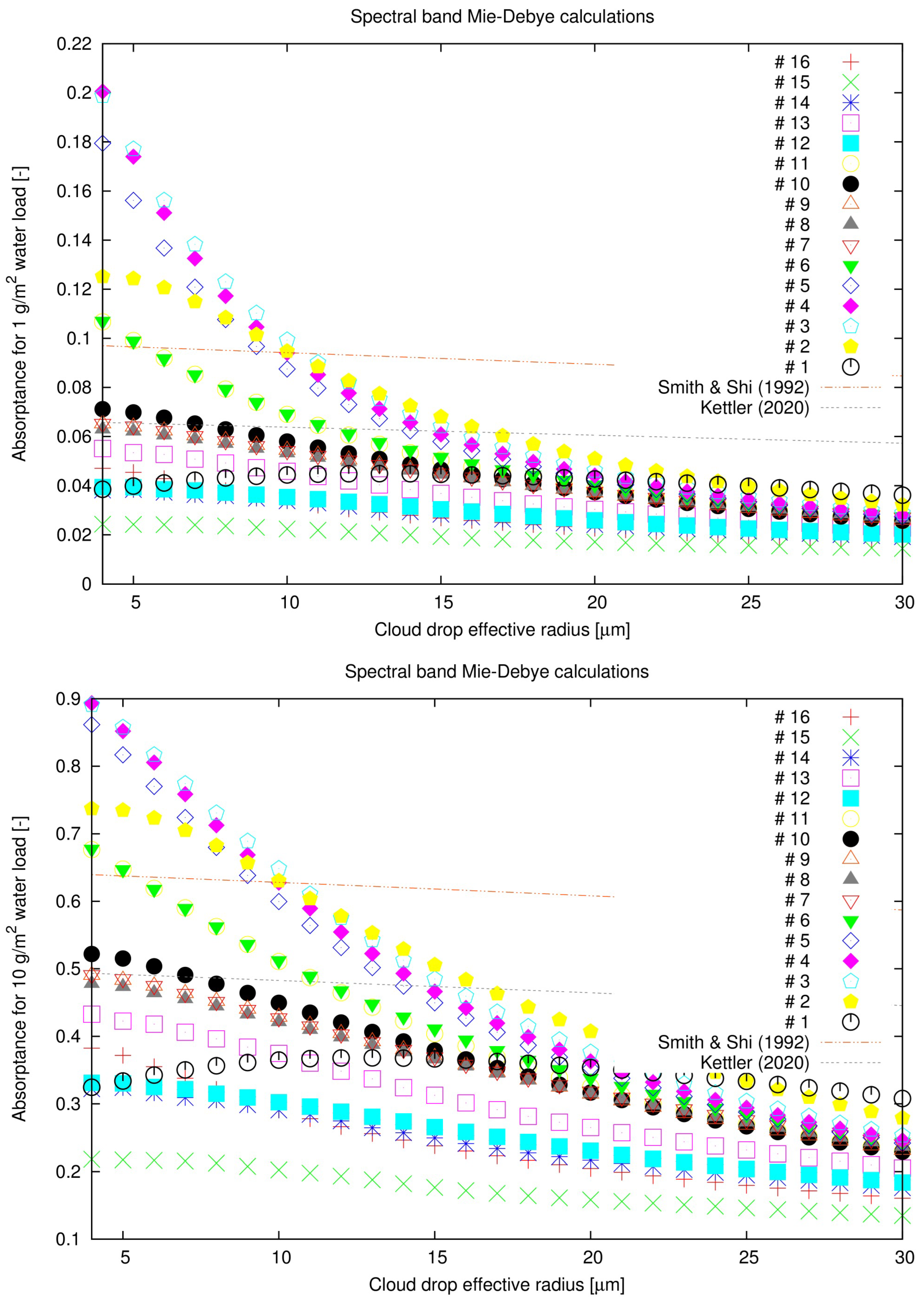

| LW band | a | b | c | d | e | f | g |
|---|---|---|---|---|---|---|---|
| 1 | -8.521E-03 | 9.341E-04 | -2.611E-05 | 2.470E-07 | 4.940E-01 | -1.496E+00 | 1.495E+00 |
| 2 | -8.737E-04 | 2.558E-04 | -2.210E06 | -2.190E-08 | 3.678E-01 | -1.879E+00 | 3.198E+00 |
| 3 | 5.902E-02 | -2.827E-03 | 7.173E05 | -6.961E-07 | -1.016E-02 | -2.569E-01 | 5.617E-01 |
| 4 | 3.365E-02 | 1.835E-03 | 4.930E05 | -4.967E-07 | 4.807E-01 | -2.564E+00 | 4.461E+00 |
| 5 | 9.855E-02 | -4.580E-03 | 1.062E04 | -9.421E-07 | -3.690E-01 | 1.214E+00 | -1.617E+00 |
| 6 | 3.752E-02 | -2.601E-03 | 6.810E-05 | -6.291E-07 | 7.428E-01 | -2.333E+00 | 2.869E+00 |
| 7 | 1.204E-01 | -5.852E-03 | 1.278E-04 | -1.045E-06 | -1.854E-01 | 5.470E-01 | -8.288E-01 |
| 8 | 9.444E-02 | -3.925E-03 | 7.286E-05 | -5.088E-07 | -7.120E-02 | 1.225E-01 | -1.504E-01 |
| 9 | 7.449E-02 | -2.699E-03 | 4.307E-05 | -2.586E-07 | 6.176E-02 | -3.441E-01 | 4.269E-01 |
| 10 | 7.749E-02 | -2.928E-03 | 5.146E-05 | -3.591E-07 | 4.441E-02 | -1.767E-01 | 6.093E-02 |
| 11 | 2.004E-02 | -1.134E-03 | 2.468E-05 | -1.993E-07 | 8.347E-01 | -2.580E+00 | 3.197E+00 |
| 12 | -5.067E-02 | 1.808E-03 | -3.382E-05 | 2.552E-07 | 1.515E+00 | -2.572E+00 | 1.520E+00 |
| 13 | -5.707E-02 | 2.044E-03 | -3.788E-05 | 2.816E-07 | 1.575E+00 | -1.810E+00 | -4.621E-01 |
| 14 | -7.484E-02 | 2.538E-03 | -4.423E-05 | 3.096E-07 | 1.882E+00 | -3.059E+00 | 4.880E-01 |
| 15 | -7.583E-02 | 1.924E-03 | -2.835E-05 | 1.873E-07 | 2.461E+00 | -1.015E+01 | 1.415E+01 |
| 16 | 7.079E-02 | -6.443E-04 | -1.294E-05 | 1.528E-07 | -2.350E-01 | 6.213E-01 | -5.661E-01 |
Disclaimer/Publisher’s Note: The statements, opinions and data contained in all publications are solely those of the individual author(s) and contributor(s) and not of MDPI and/or the editor(s). MDPI and/or the editor(s) disclaim responsibility for any injury to people or property resulting from any ideas, methods, instructions or products referred to in the content. |
© 2024 by the authors. Licensee MDPI, Basel, Switzerland. This article is an open access article distributed under the terms and conditions of the Creative Commons Attribution (CC BY) license (http://creativecommons.org/licenses/by/4.0/).


