3. Methodology
The dataset we used is Wood Defection dataset [
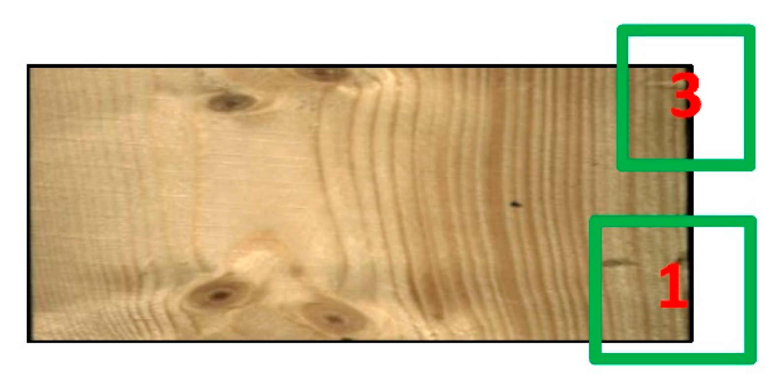
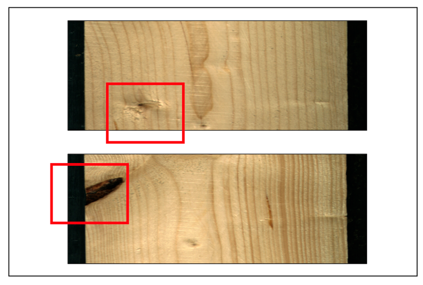
3]. It contains 4000 images with annotation for wood surface defects of different types. Some of the examples include No Defect and defect (Quartzity, Live knot, Marrow resin, Dead knot, knot with crack, knot missing and Crack). The original dataset had high resolution images captured with special camera which takes up to 12MB of disk space per image. The size of the dataset has been reduced by resizing the images to 256*256*3 (196608 features). The dataset contains YOLOv5 annotations, which contains the bounding boxes and respective labels as shown in the
Figure 1a.
Figure 1.
Image with Bounding Boxes and Labels.
Figure 1.
Image with Bounding Boxes and Labels.
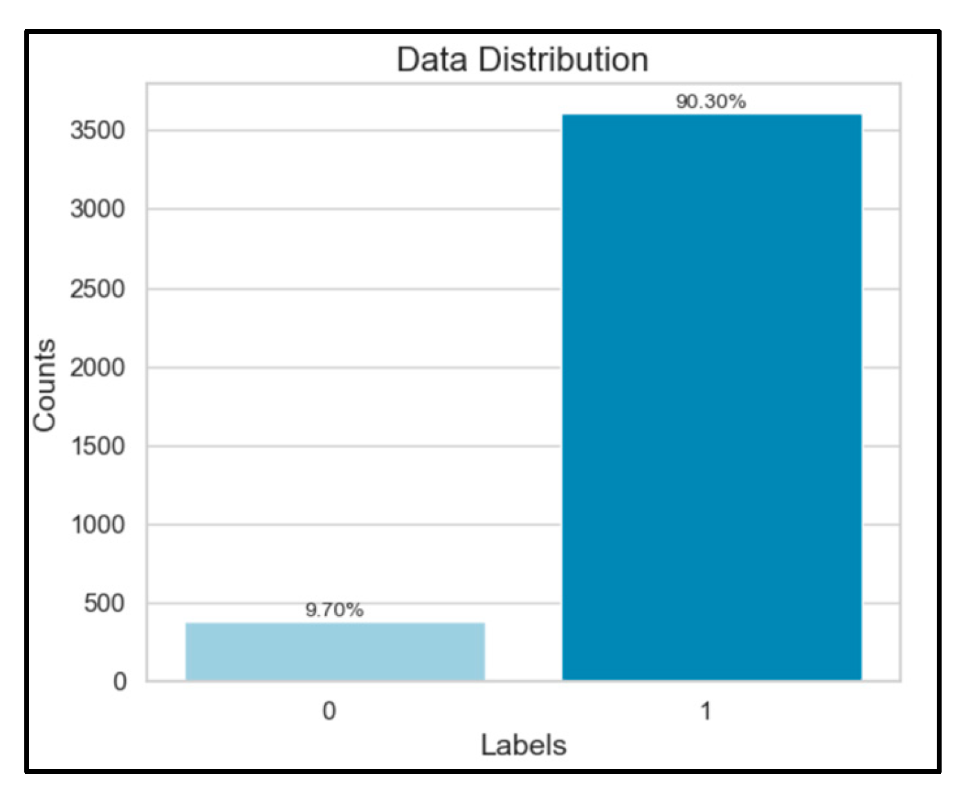
To tackle the imbalanced nature of our dataset, we framed the task as a binary classification problem focused on detecting defects in wood surfaces. The dataset's structure relies on bounding boxes, where Class 0 signifies defect-free surfaces, and Class 1 denotes defective ones. However, Class 1 instances are approximately one-tenth the number of Class 0 instances, posing a significant challenge due to potential bias towards the majority class.
Figure 2.
Data Distribution in Original Data.
Figure 2.
Data Distribution in Original Data.
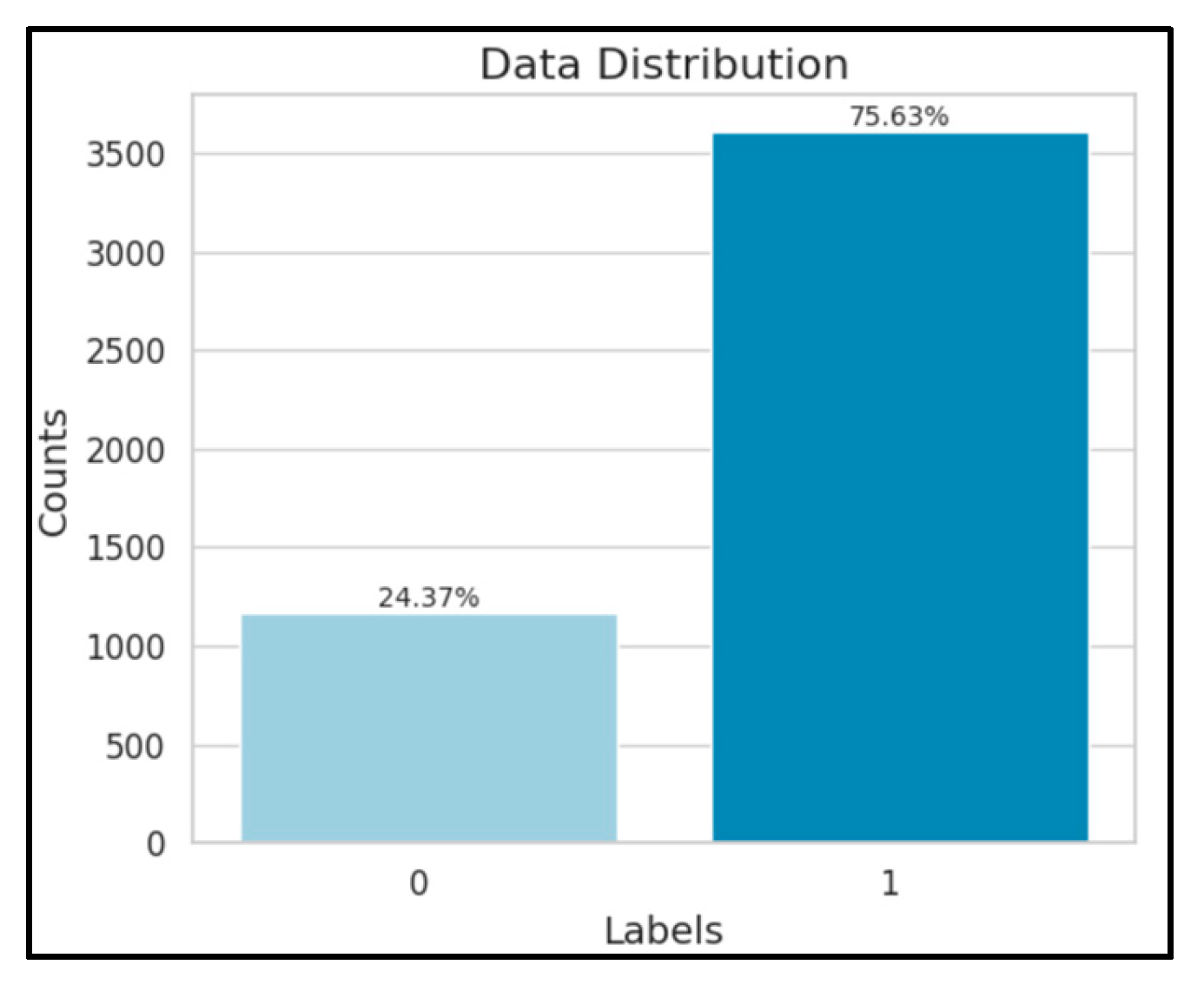
To mitigate this, we utilized Random Over-Sampling, duplicating Class 0 instances to balance representation during training. This strategic augmentation aimed to foster a more equitable distribution, enhancing the model's ability to accurately identify both defective and non-defective wood surfaces and ensuring robustness in classification.
Figure 3.
Data Distribution in Oversampled Data.
Figure 3.
Data Distribution in Oversampled Data.
Data preprocessing included several key steps to ensure optimal model performance. Images were resized to 256x256x3 using Lanczos interpolation, a method chosen for its ability to preserve image quality and sharpness. We also converted the images to the RGB color space, which is well-suited for display on screens and has shown to train effectively. For normalization, each image was standardized by subtracting the mean and dividing by the standard deviation of the training set, with these values saved for use during prediction. Additionally, categorical target variables were converted to numerical values using one-hot encoding, transforming them into binary vectors that facilitate the training of our machine learning model.
In our approach, we integrated several renowned pre-trained models to enhance feature representation and model performance. ResNet50, a deep neural network known for its capacity to efficiently capture intricate image features, formed the basis of our architecture, facilitating the detection of subtle details in wood surfaces. Additionally, we employed the AlexNet architecture, which is celebrated for its pioneering design in computer vision, enabling effective pattern recognition and defect detection on wood surfaces.
Further, we utilized EfficientNetB7 for its efficiency and scalability, which strikes a balance between computational resources and accuracy in capturing detailed patterns from wood surfaces. VGG19 also played a crucial role in our approach; its deep architecture and robust feature extraction capabilities made it the top performer, leading us to select it as our preferred model. This model, trained on extensive datasets like ImageNet, allowed us to fine-tune our approach for specific tasks, such as defect detection in wood, by using transfer learning to handle the challenges posed by our imbalanced dataset.
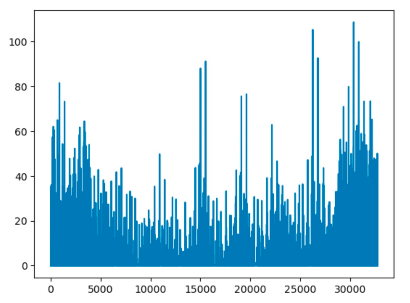
Figure 4.
Feature Representation of an Image by VGG19.
Figure 4.
Feature Representation of an Image by VGG19.
We then applied feature reduction techniques to evaluate performance enhancements.
Principal Component Analysis (PCA) was used to streamline the feature space. This linear dimensionality reduction technique identified and preserved essential features by projecting data onto orthogonal axes, or principal components. While attempting to balance computational simplicity and information retention necessary for accurate defect detection, the highest accuracy achieved using PCA configurations suggested its limited effectiveness for our specific dataset, with an accuracy of 85.35% and an F-1 score of 0.8594.
To address non-linear relationships in the data, we implemented Kernel Principal Component Analysis (Kernel PCA), which utilizes kernel functions to map data into a higher-dimensional space, aiding in the extraction of complex patterns. Despite efforts to optimize kernel parameters, the top accuracy reached with Kernel PCA also indicated limited success, recording an accuracy of 85.96% and an F-1 score of 0.8646.
The modest performance of both PCA and Kernel PCA could be attributed to several factors: potential loss of crucial information due to dimensionality reduction, increased risk of overfitting where reduced dimensions may not generalize effectively to new data, and the provision of dense solutions that might obscure vital features by including all in the transformed space. These factors collectively could undermine the effectiveness of these techniques in enhancing our defect detection model.
In our continuous quest to enhance the performance, we explored feature learning techniques with a specific focus on sparse modeling, a pivotal aspect of our goals. Contrary to the expected improvement, feature reduction techniques did not yield the desired enhancements in performance. As a strategic pivot, we shifted our attention to sparse modeling techniques, aiming to selectively emphasize relevant features by inducing sparsity in the feature space. Two prominent sparse modeling techniques were implemented: Lasso regularization and Elastic Net regularization. The rationale behind employing sparse modeling was to accentuate the significance of relevant features while mitigating the impact of irrelevant ones. By designating certain features as sparse (assigned a coefficient of 0), these techniques enabled the identification and prioritization of crucial information for wood surface defect detection [
2]. This strategic shift toward sparse modeling reflects our commitment to adapt and refine our approach based on empirical results, ultimately steering the project toward its primary goal of efficient and accurate defect detection in wood surfaces.
Lasso Regularization:
Lasso regularization serves as a potent tool in preventing overfitting, a common challenge in machine learning models. Its mechanism involves augmenting the standard least square’s objective function with a penalty term proportional to the absolute values of the coefficients within the regression model as shown in the Equation (1). This added L1 penalty induces sparsity in the model by driving certain coefficients to exactly zero. In the context of our wood surface defect detection project, we applied Lasso regularization to optimize the cost function, which includes both the least square errors and the L1 penalty term. During the training phase, where the model learns from labeled data, the objective is to minimize this cost function. This process entails determining the coefficients that minimize the combined impact of least square errors and the L1 penalty [
4]. These coefficients, once identified through the training process, are then employed to predict features in testing instances. The regularization parameter, denoted as lambda, plays a pivotal role in governing the strength of regularization. A higher value of lambda indicates more potent regularization, effectively emphasizing sparsity in the model. This fine-tuning parameter allows us to strike a balance between fitting the model to the training data and preventing it from becoming overly complex, thereby contributing to robust and effective defect detection in wood surfaces.
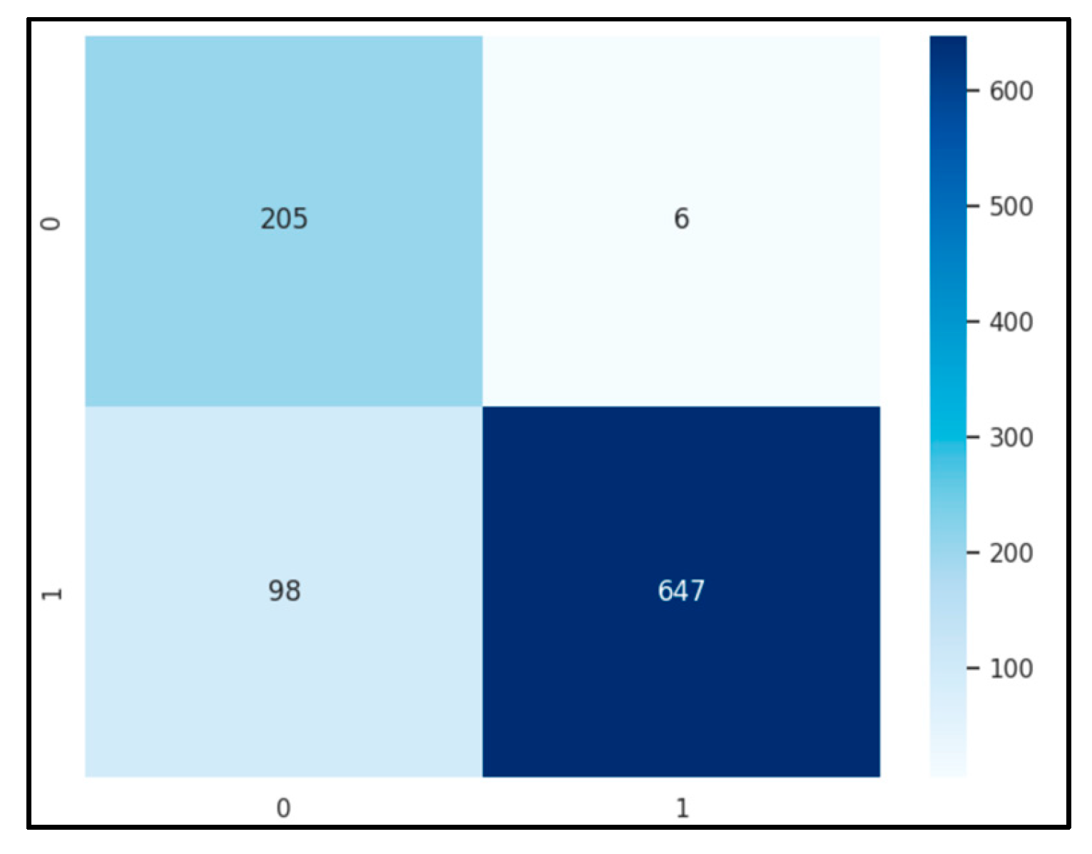
The Lasso regularization was implemented using the library from scikit-learn. Setting the regularization constant (Lambda) to 0.01, the application of Lasso regularization resulted in a notable reduction of features for each image. Specifically, the feature count diminished from 32,768 to 2,026, signifying a substantial simplification of the dataset. The efficacy of this reduction lay in its ability to retain relevant information while discarding less significant features. The refined set of 2,026 features was then employed to train and fit a KNN model. This sequential approach not only facilitated computational efficiency but also aimed to enhance the model's performance by focusing on the most informative attributes derived through Lasso regularization.
Accuracy: 89.12%
F-1 score: 0.8974.
Figure 5.
Confusion matrix of Lasso Features using KNN.
Figure 5.
Confusion matrix of Lasso Features using KNN.
Elastic Net Regularization:
Elastic Net regularization [
8], a hybrid approach encompassing both L1 and L2 regularization, offers a nuanced solution by striking a balance between the sparsity-inducing nature of Lasso and the grouping effect of Ridge as shown in equation (2). In our implementation, we set the hyperparameters to an alpha value of 0.01 and an L1_ratio of 0.5, signifying equal importance given to both Lasso and Ridge regularization. Notably, a L1_ratio of 1 emphasizes Lasso, while 0 emphasizes Ridge, allowing us to fine-tune the regularization strategy based on the characteristics of our data. Remarkably, our experimentation with Elastic Net yielded results comparable to those obtained with Lasso in terms of selected features and performance scores. However, the similarity in results suggests that the functionality of Ridge, a prominent component of Elastic Net, might not be particularly suitable for our specific case. Ridge regression is particularly beneficial when dealing with datasets that exhibit highly correlated features. In our context, the dataset might lack such high correlations, potentially rendering the Ridge component less impactful. The adaptive nature of our approach acknowledges the nuances of our dataset, underscoring the importance of tailored regularization strategies to optimize the performance of our wood surface defect detection model.
Optimization:
With a streamlined dataset refined through Lasso regularization, our project pivoted towards optimization strategies to boost efficiency and predictive accuracy. We integrated the proximal gradient optimization technique to fine-tune feature representation, enhancing model performance. This advanced strategy goes beyond traditional methods by adjusting features refined through Lasso regularization, aiming to balance sparsity with accuracy—these aid in retaining essential information while minimizing extraneous details.
We employed the proximal gradient descent method specifically on Lasso features, using the following objective function equation.
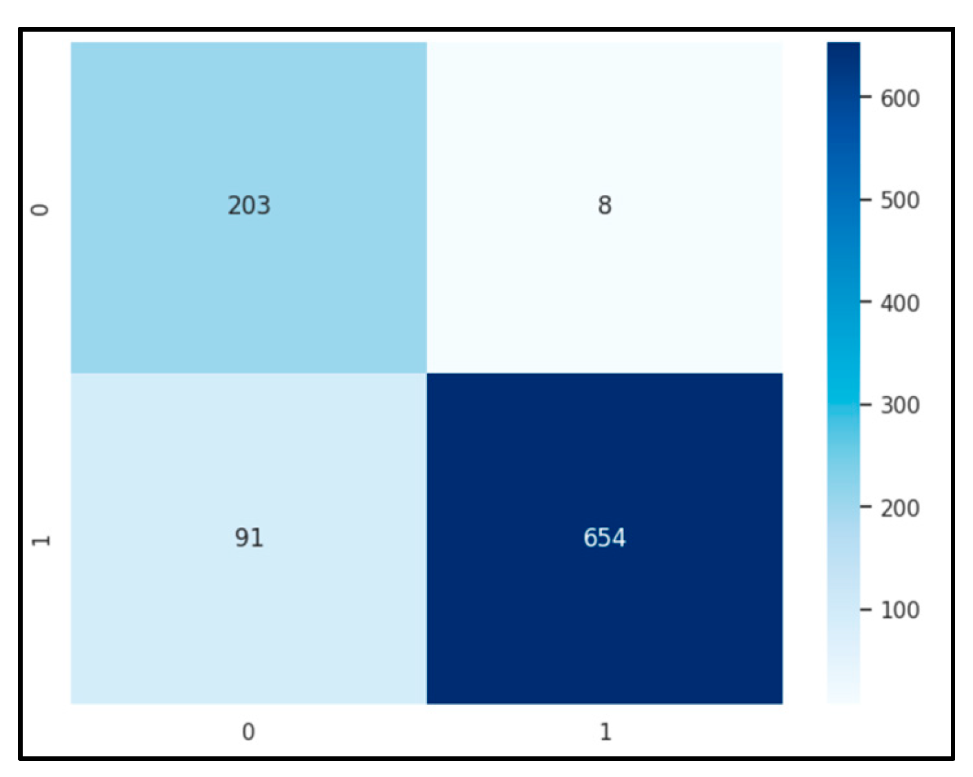
The training targets, with λ set at 0.1. Optimization was facilitated by the L-BFGS-B algorithm from the SciPy library, which is tailored for bound-constrained optimization, ensuring coefficients stay within defined bounds. After 10 optimization cycles, we significantly reduced the feature set from 32,768 to just 1,179, maintaining robust performance with an accuracy of 89.65% and an F-1 score of 0.902.
Figure 6.
Confusion matrix of Proximal Gradient Features using KNN.
Figure 6.
Confusion matrix of Proximal Gradient Features using KNN.
The combination of Lasso regularization and proximal gradient optimization provides considerable benefits, particularly in handling high-dimensional datasets. These techniques not only enhance feature selection and model interpretability but also increase computational efficiency. By promoting sparsity, where non-essential features are driven to zero, these methods refine the feature set, thereby improving the model's predictive accuracy and ensuring a streamlined, efficient modeling process.
