1. Introduction
The photovoltaic (PV) installed capacity grows exponentially to meet the decarbonation goals of the electric sector [
1]. The global photovoltaic (PV) installed capacity, vital for the electric sector decarbonation, has reached 1,552.3
in 2023. In France, the capacity stood in April 2024 at 19.9
. The growth of the PV installed capacity over a year was nearly 32% worldwide and 15.7% in France [
2,
3]. The integration of these amounts of PV electricity into the grid is challenging as transmission system operators (TSOs) lack measurements of the
rooftop PV
1 power production, which currently represents about 20% of the PV installed capacity in France [
4]. This so-called problem of poor PV observability threatens the integration of PV into the grid as inaccurate estimations of the PV power measurements could lead to issues in grid management such as imbalances, congestions or increased power reserves requirements [
4,
5].
The poor rooftop PV observability originates from two main factors. First, TSOs have little information on the small systems located on the distribution grid (which corresponds to rooftop PV systems [
6,
7]). Second, they lack ground truth measurements of the PV power production generated by rooftop PV systems. This prevents them from assessing the accuracy of PV power generation estimation methods leveraged by TSOs to estimate the PV power production of installations for which measurements are unavailable.
In recent years, numerous works have proposed using deep learning [
8] and airborne or satellite imagery to map rooftop PV systems. Many regions, especially in Europe and in the United States, have been mapped [
7,
9,
10,
11,
12,
13,
14,
15,
16,
17]. These mappings are increasingly detailed as recent works such as [
13] or [
12] construct PV registries gathering the localization, tilt and azimuth angles and installed capacities of individual PV systems. As underlined by [
18], these characteristics are sufficient to estimate the PV power production using a conversion model and weather data.
In this work, we leverage a large dataset of PV power measurements of rooftop PV systems provided by the non-profit association
Asso BDPV to evaluate whether estimations of the PV power production using information consolidated in remote sensing-based rooftop PV registries enable an
accurate estimation of the rooftop PV power production. Our central contribution is to show that we can derive fair estimations of the PV power production at the individual system scale using the vanilla conversion model PV Watts [
19], weather data and the PV system’s characteristics recorded in remote sensing-based rooftop PV registries such as those proposed by [
20] or [
13]. This work demonstrates that we can overcome the poor rooftop PV observability by combining limited information on the PV systems obtained from Earth observation data and remote sensing techniques with weather data, using off-the-shelf conversion models.
2. Background and Related Works
2.1. Background: The Poor Observability of Rooftop Photovoltaic Systems
Wind and solar PV electricity generation is weather-dependent and variable at different time and space scales. Large wind and PV penetration increases the grid’s sensitivity to climate and forecasting uncertainties. To limit the uncertainties they bring to the grid, it is necessary to accurately observe (i.e., accurately measure or estimate) their power production. We define observability as the ability of the TSO to accurately estimate a power unit’s real-time production. We say that a power unit is observable if the TSO can directly measure its production (by having access to real-time telemetry) or derive accurate estimations of the power production, e.g., based on ex-post measurements (usually available within a month).
Accurate measurements of renewable power generation at the scale of the power units are the basis for validating short-term forecast models, which use weather forecasts to estimate future renewable power production and the power system’s margins necessary to compensate for the variability of the effective production. Wind power generation is well observed [
4], but this is not the case for all types of PV power production. Indeed, a distinctive feature of PV energy is that PV installations vary in size. The smallest PV power installations have a few
installed capacity. In contrast, the largest plants can have an installed capacity of up to several hundreds of
—the variability in size results in a great diversity in terms of the installations’ technical characteristics (e.g., PV module efficiency and orientation, presence of a solar tracker). This diversity in the system’s characteristics makes the extrapolation from larger (and well-measured plants) to smaller plants inaccurate.
Table 1 summarizes the current state of PV observability in France, depending on whether the TSO has at least access to
ex-post measurements, depending on the categories of installed power capacity. Overall, about 94% of the PV fleet is not observable, corresponding to 22% of the installed capacity, roughly equivalent to four 900 MW nuclear units. The lack of observability primarily concerns small-scale installations with installed capacity below 36
.
The lack of observability will be increasingly concerning in the context of the quick growth of PV installed capacity. We expect the overall French PV installed capacity could reach up to 200
in 2050 [
21]. The
Programmation pluriannuelle de l’énergie (PPE, [
22])
2 aims to reach between 35 and 45
of PV installed capacity by 2029 [
22]. These scenarios and objectives assume a constant deployment rate for small-scale and large PV, meaning that up to 40
(i.e., two-thirds of the current French nuclear park’s capacity) could be unobserved by 2050 with the current practices. Therefore, improving the observability of small-scale rooftop PV systems (i.e., PV installations with an installed capacity below 36
) is crucial.
2.2. Related Works
2.2.1. Regional PV Power Estimation and Forecast
As depicted in
Table 1, in September 2023, 661 241 installations, amounting to 3.7
(i.e., 22% of the French PV installed capacity at that time) are not observed, meaning that we have neither telemetry nor
ex-post measurements of their production.
The traditional way of estimating the production of PV power units when telemetry is unavailable is to resort to
regional PV power modeling approaches. The upscaling approach [
23] consists in estimating a capacity factor (i.e., a value between 0 and 1 corresponding to the ratio between the the actual electric production over a period and the one that would be produced with the total installed capacity over the same period) based on the PV power production of metered neighboring reference plants and imputing this capacity factor to a set of unmetered plants, for which only the installed capacity is known. Regarding their technical characteristics, the reference plants may not represent the target plants, so interpolation errors arise [
24]. To overcome this difficulty, the probabilistic approach [
18] proposed using a physical PV system model and solar irradiance data instead of neighboring plants. Indeed, only a few parameters are necessary to estimate the PV power production of a system. However, it is necessary to acquire these parameters. [
18] showed that in addition to its
localization, the
tilt and
azimuth angles, and the
nameplate capacity (or installed capacity) of the PV installation are sufficient.
The probabilistic approach can be expanded to all power classes of PV power systems and could, in principle, address the lack of observability of rooftop systems. However, contrary to power plants for which the technical characteristics can be accessible or derived from optimal parameters, the characteristics of the rooftop PV power systems (whose installed capacity is lower than 36
are generally not available [
7] and have no reason to be optimal as they depend on the built environment. Also, reference power measurements from these small installations, necessary to validate the PV power estimation method’s accuracy, are generally unavailable.
2.2.2. Remote Sensing of Rooftop PV Systems
The lack of knowledge regarding the geographical distribution and the technical characteristics of small-scale PV installations’ is a recurring problem in many countries [
6,
7]. We refer the reader to the literature reviews of [
25,
26], and [
15] for an exhaustive presentation of work on the subject. Early works on the topic focused on building databases containing annotations of installations on orthoimages
3 [
27] and on assessing the feasibility of a remote sensing-based method to identify PV systems [
6,
28]. Authors investigated methods involving manually calculating statistics for each pixel and classifying pixels according to these statistics [
28,
29,
30,
31,
32] and methods using deep convolutional networks [
7,
33,
34,
35,
36,
37]. The performance of these algorithms is evaluated with the F1-score.
4, and comparative studies have shown the superior performance of algorithms using convolutional networks over those based on manual extraction of image statistics. For example, the method of [
28] achieves an F1 score of just 0.6, while [
7] exceeds 0.8.
The DeepSolar project [
9] marked a significant milestone for mapping small-scale PV installations from orthoimagery. This work relied on deep convolutional networks to detect installations and estimate their surface area. This model was deployed across the United States of America, and the authors reported an error in area estimation of less than 5%
5. DeepSolar and follow-up implementations have been used to map regions and countries, especially in Europe: The Netherlands [
38], Western Germany [
39], Sweden [
10,
11], Northern Italy [
15] or France [
12].
The latest works on the topic propose methods to construct registries that record the localization and surface area of the PV systems, as well as their tilt and azimuth angles and their installed capacity. [
13,
41] leveraged 3D-building data in addition to orthoimagery to estimate the tilt and azimuth angles of the PV systems located in North-Rhine Westphalia. On the other hand, [
12] leveraged the small-scale PV registry maintained by the non-profit association
Asso BDPV and the Python package
PyPVRoof [
42] to estimate the tilt and azimuth angle over France, without requiring 3D data.
To map PV systems in France, [
12] leveraged DeepPVMapper [
40], a mapping algorithm that improves upon [
13] to map and characterize rooftop PV installations.
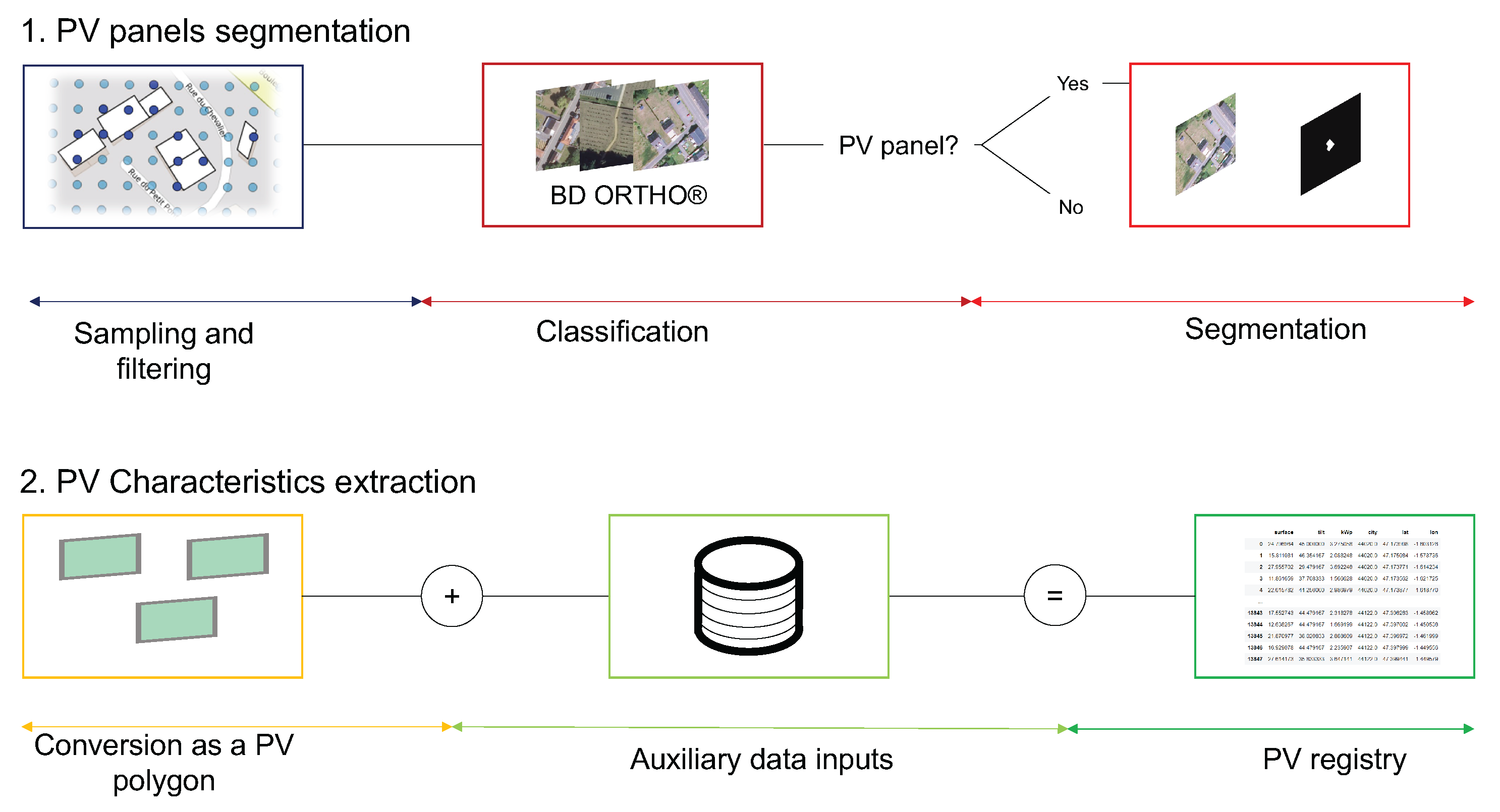
Figure 1 summarizes the workflow of DeepPVMapper. Firstly, geolocated PV installation polygons are extracted from orthoimages using image classification and segmentation models. Second, these polygons and a survey of characteristics of PV installations are used to infer the PV installations’ characteristics (tilt, azimuth, installed capacity).
2.2.3. Estimation of the Power Production of Rooftop PV Systems
The registries of rooftop PV systems obtained using Earth observation data and deep learning cannot be directly used to infer the power production of these systems. Indeed, one needs ground truth power measurements to evaluate the accuracy of the estimation of the PV power production computed using data coming from these registries. Such measurements are not systematically registered, and if they are, they are often kept private for privacy or commercial reasons. Only a few works have had access to individual rooftop PV power curves. For instance, [
43] used PV systems measurements for 740 systems (at a time resolution of 5 minutes) of businesses and homes in Western Australia. Their approach consisted in a spatial polynomial interpolation of the PV power production of measured homes to estimate the PV power production of the unmetered systems, whose locations and sizes were known thanks to PV registries. [
24] had access to only a few tens of power measurements for systems with an installed capacity lower than 36
[
44] used the Pecan Street’s Dataport [
45], which contains measurements at a 1-minute resolution for 73 households across the United States of America. [
44] focused on forecasting, introduced an ensembling method to forecast the PV power production, and tested their method on the rooftop PV power production forecast. The forecast models included in their ensembling approach are autoregressive models fitted on past power curves.
Finally, [
46] leveraged data from IBW, the local utility of Wohlen in Switzerland. This dataset contains PV power generation profiles of 15 homes and the PV systems’ technical characteristics. They introduced an approach to derive hourly PV generation using the information on the localization and surface area of PV systems.
[
46] is the closest work to ours, as their approach does not require prior access to PV power curves for fitting estimation of forecast models. However, they did not explicitly model the PV systems; they only relied on estimating geographical, physical, and technical potentials, yielding an overestimation of hourly power generation. Our approach shows that by leveraging barely more information on the PV systems, we can accurately estimate the individual rooftop PV power production using proper modeling of the PV systems. Our study also spans a much larger geographic area and leveraged more rooftop PV systems than theirs.
3. Data
3.1. Ground Measurement Data: Individual Rooftop PV Yield Time Series
3.1.1. Overview
Thanks to the non-profit association
Asso BDPV, we had access to ground truth PV power production measurements of 1,793 individual PV systems. These systems correspond to a subset of those featured in the training dataset BDAPPV [
47]. These measurements span mainland France and have a time resolution of 30 minutes.
This means that with these measurements, we have all the necessary information to carry out rooftop PV power estimation, from detecting the installation on aerial images to estimating the accuracy of the power production estimation. We also know the precise location of the installations, contrary to [
43], who relied on postcodes.
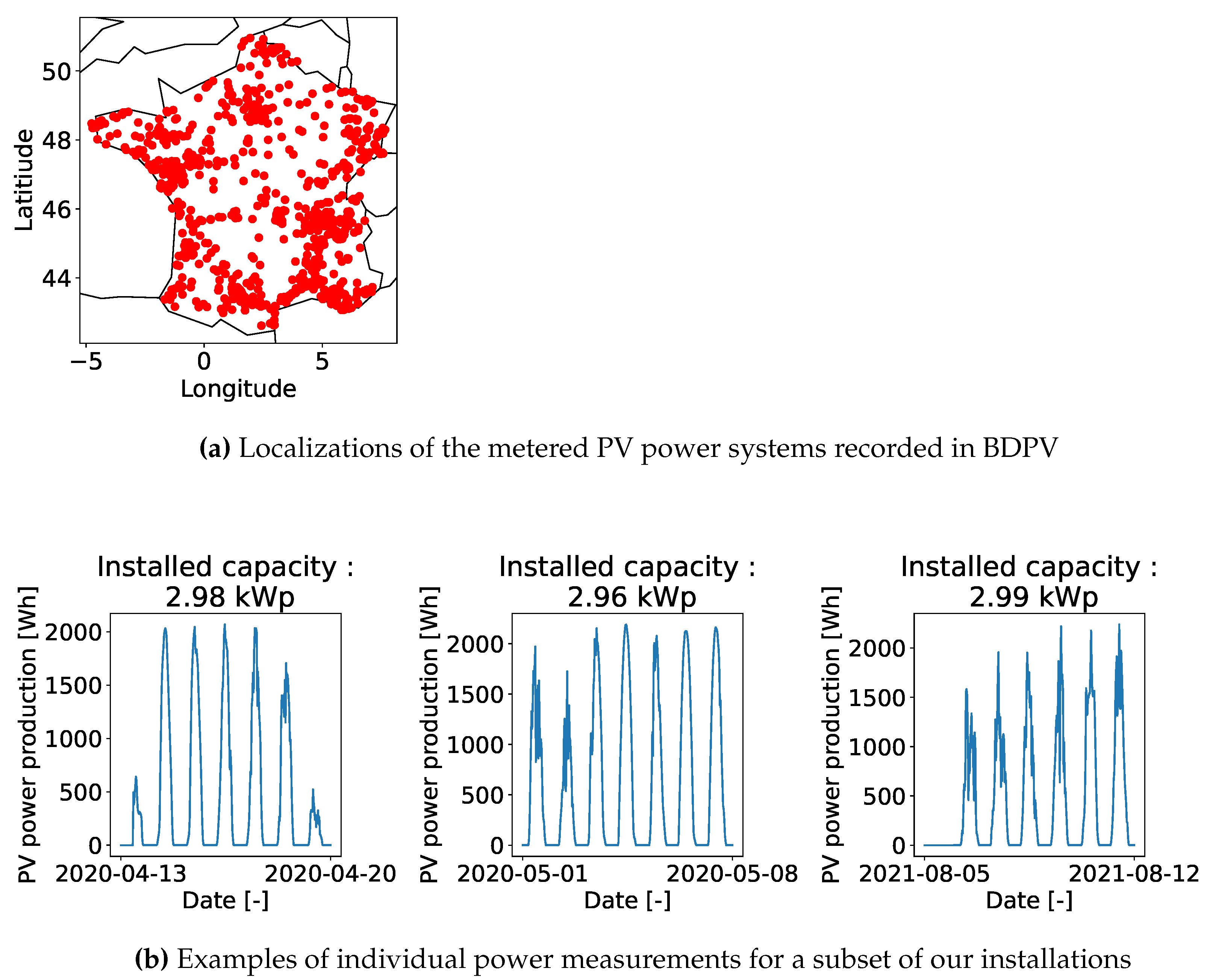
Figure 2 plots the localization (
Figure 2a) of the PV measurements and examples (
Figure 2b) of power output time series coming from our dataset.
3.1.2. Quality Checks
BDPV enables its users to assess the quality of the production of their PV installation. We refer the reader to [
48] for a detailed description. We leveraged this quality assessment report to filter out faulty measurements. In addition to this filtering, we matched the PV yield time series corresponding to a single installation in the BDAPPV database. Of the 1,793 raw installations, 906 passed our quality checks and filters. We refer the reader to
Appendix B for examples of production reports leveraged to filter the faulty measurements and to [
47] for a description of the matching procedure between the annotations on aerial images and the actual PV systems. Examination of the filtered installation showed that we kept installations spreading over France (see
Figure 2a).
On our curated dataset, we have, on average, 27,346 measures per installation, corresponding to an average duration of 569,7 days of observations. The time window spans from December 2, 2020, to February 15, 2023.
3.2. PV Registry
We consider the PV registry generated with DeepPVMapper. At the time of writing, this registry contains more than 100,000 installations. However, in this study, we aim to evaluate the data quality to estimate rooftop PV power production. Therefore, we focus on detections for which we have ground truth characteristics. This corresponds to installations coming from BDPV, which are part of the testing dataset of DeepPVMapper. We have 1,485 installations in the test set of DeepPVMapper, which we intersect with the 904 clean power measurements. We end up with 276 unique installations.
Table 2 presents some descriptive statistics of the PV registry used in this registry. Note that we refer to as "ground truth characteristics" the system’s characteristics that were imputed by the owners of the systems registered in the BDPV database.
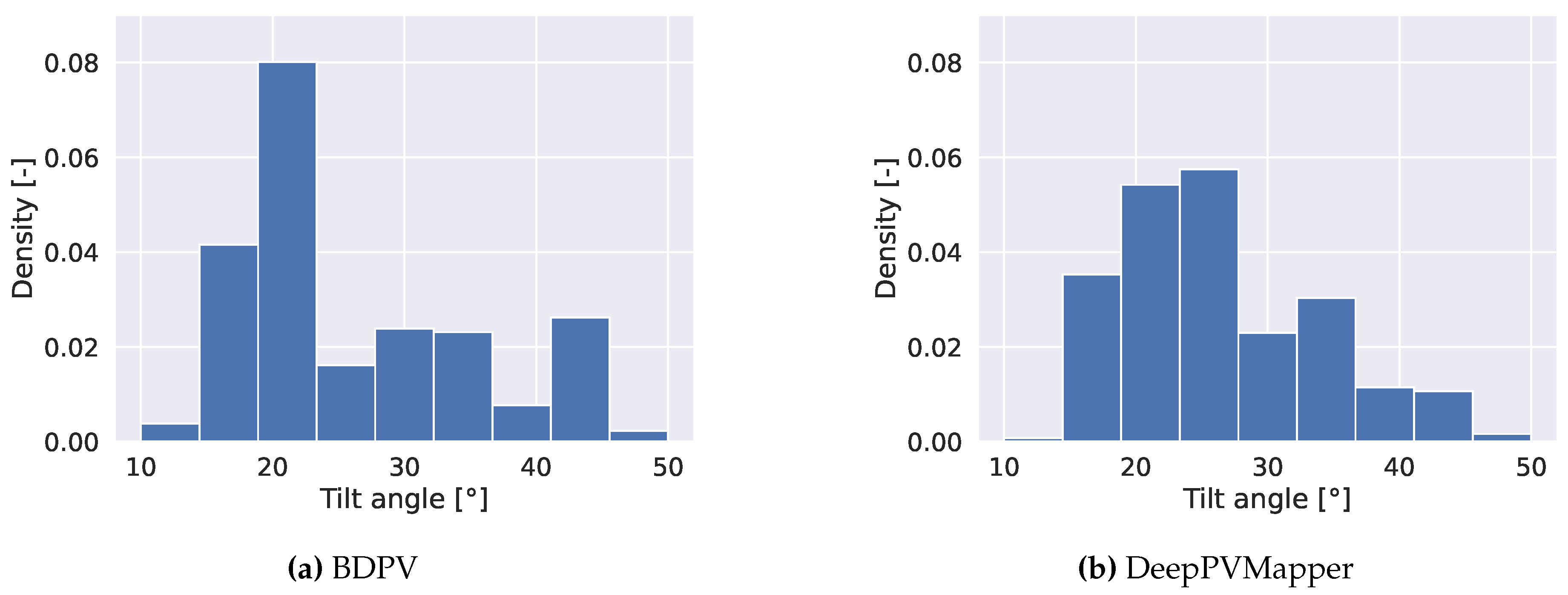
Figure 3 presents the distribution of the tilt angle for these installations, as recorded in BDPV (
Figure 3a) and estimated by DeepPVMapper (
Figure 3b). We can see that the tilt angle estimation by DeepPVMapper is flatter than the distribution recorded in BDPV. This is because the imputation of the tilt angle by DeepPVMapper is the mean tilt angle around the location of the PV panel.
3.3. Solar Radiation and Temperature Data
3.3.1. Solar Radiation Data
The Copernicus Atmospheric Monitoring Service (CAMS, [
49]) solar radiation services provide all-sky historical values (2004 to present) of global (GHI), direct (BHI), and diffuse (DHI) solar irradiation, as well as direct normal irradiation (BNI). The services also provide the coincident clear-sky irradiance components (GHI, DHI, BNI) for (underlying) clear-sky conditions. Solar radiation is retrieved from the Meteosat Second Generation (MSG) satellite observations (SEVIRI sensor). These clear-sky irradiance estimations are obtained using aerosol, ozone, and water vapor information from the CAMS global forecasting system. The database covers the Field of View of Meteosat ranging from -65° to 65° North-South and East-West directions, comprising metropolitan France with a nadir (directly below the satellite) spatial resolution of 3 km and a temporal resolution of 15 minutes. In the following, we consider the 30-minute averaged values for a time interval between 2020 and 2023. The spatial location of the irradiance values encompasses to the pointwise location, which is estimated by DeepPVMapper.
3.3.2. Temperature Data
We extract the 2-m air temperature data from ERA5 [
50], the fifth reanalysis of the European Centre for Medium-Range Weather Forecasts (ECMWF), provided via the Copernicus Climate Change Services (C3S). We only use the 2-m air temperature for a single latitude and longitude point and at a temporal resolution of 1 hour (linearly interpolated to get a temperature value every 30 minutes).
4. Methods
Our method for estimating rooftop PV power production at the individual installation level relies on the registry, solar irradiation, and air temperature data introduced in
Section 3.2 and
Section 3.3. The PV system’s characteristics and the weather data are inputs to a conversion model introduced in
Section 4.1, which returns an estimation of the DC power production of the PV system.
In
Section 4.2, we present our methodology to assess the accuracy of these estimations of the PV power production compared to the ground truth measurements (introduced in
Section 3.1).
4.1. Physically Based Solar Irradiation-to-Electric Power Conversion Model
4.1.1. Model Choice
We use the conversion model PVWatts [
19]. PVWatts considers a limited set of parameters, as displayed in
Table 3. In this study, we considered [
19] because it is one of the simplest model from the literature. Remote sensing-based registries contain little data on the individual PV systems compared to the standards for PV power simulation, so we picked a simple conversion model, which requires very limited information about PV installations.
4.1.2. Formalization
PV Watts takes as input the effective plane-of-array (POA) irradiance
and the module temperature
and returns the DC power
of the module for a given time
t. The effective POA irradiance corresponds to the POA irradiance, taking into account the optical losses of the module. These losses are accounted for following the method of [
51,
52,
53]. The computation of the POA irradiance requires knowing the module’s tilt and azimuth angle. We refer the reader to
Appendix A for more details on the computation of the POA irradiance, the module temperature, and the effective POA irradiance. Equation (
1) summarizes the conversion model,
where
is a function of the tilt angle
and the azimuth angle
of the installation,
is the installation’s installed capacity and
is an efficiency factor that reflects the decrease in the module’s performance with the temperature
.
corresponds to the temperature under the standard test conditions and is set to 25°C, and
to -0.002
.
denotes the irradiance under standard test conditions (STC) and is equal to 1000
.
4.2. Evaluation Criteria
4.2.1. Evaluation Metrics
4.2.1.1. Quantitative Metrics
Throughout our study, we evaluated the rooftop PV power yield estimation accuracy using the root mean squared error (RMSE) and the percentage RMSE (pRMSE). We define the RMSE as
where
is the estimated target value (e.g., PV power production in W),
is the true value, and
n is the number of temporal samples. Besides, we define the pRMSE as
where
j is the index of the PV system that we consider. In other words, the pRMSE is the RMSE normalized by the installed capacity. The pRMSE also corresponds to the normalized RMSE (nRMSE). We recall that we do not evaluate the accuracy of the weather data or the accuracy of the rooftop PV mapping model. For the latter, we refer the reader to [
12].
4.2.1.2. Spatio-Temporal Analysis of the Error
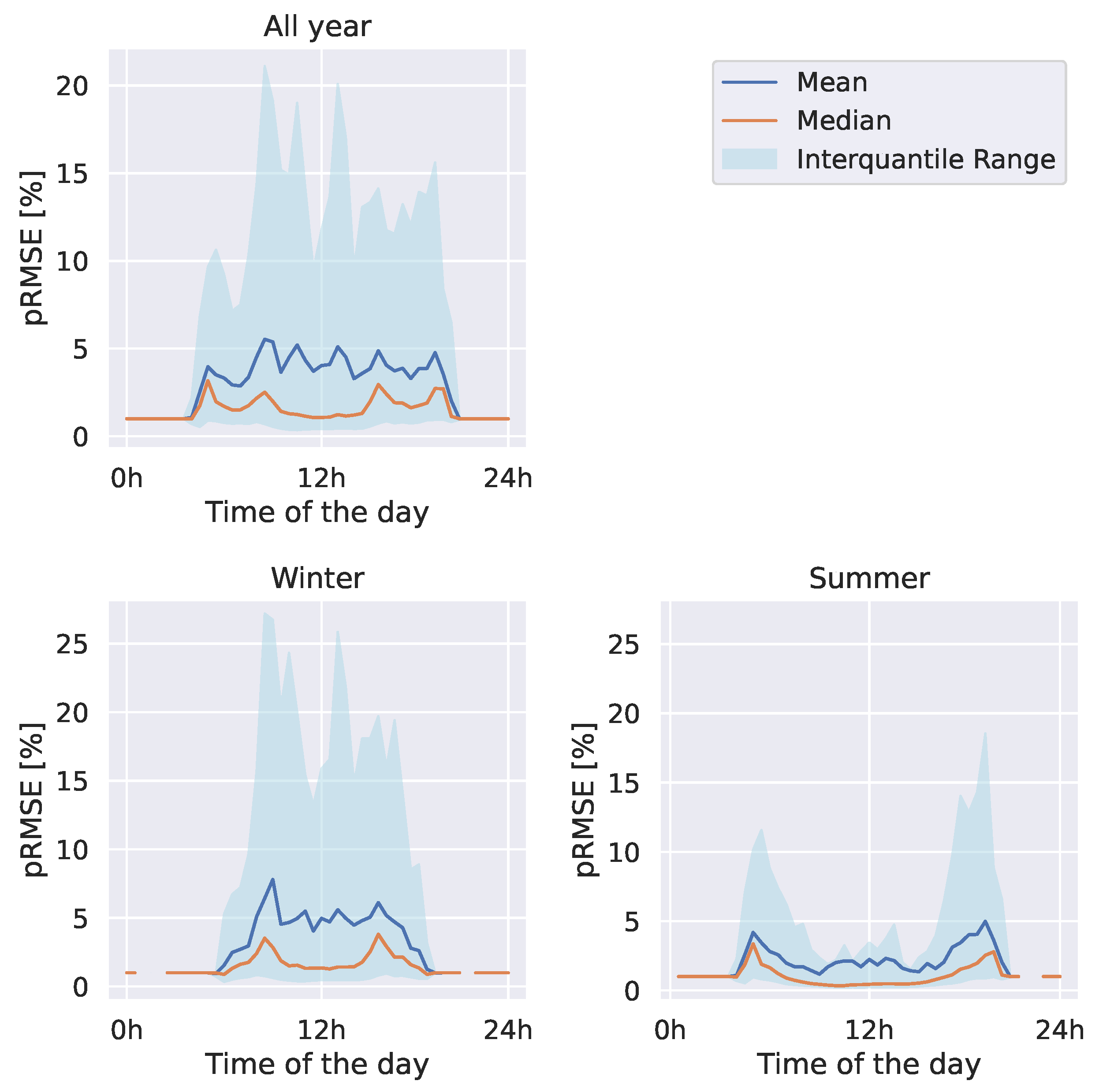
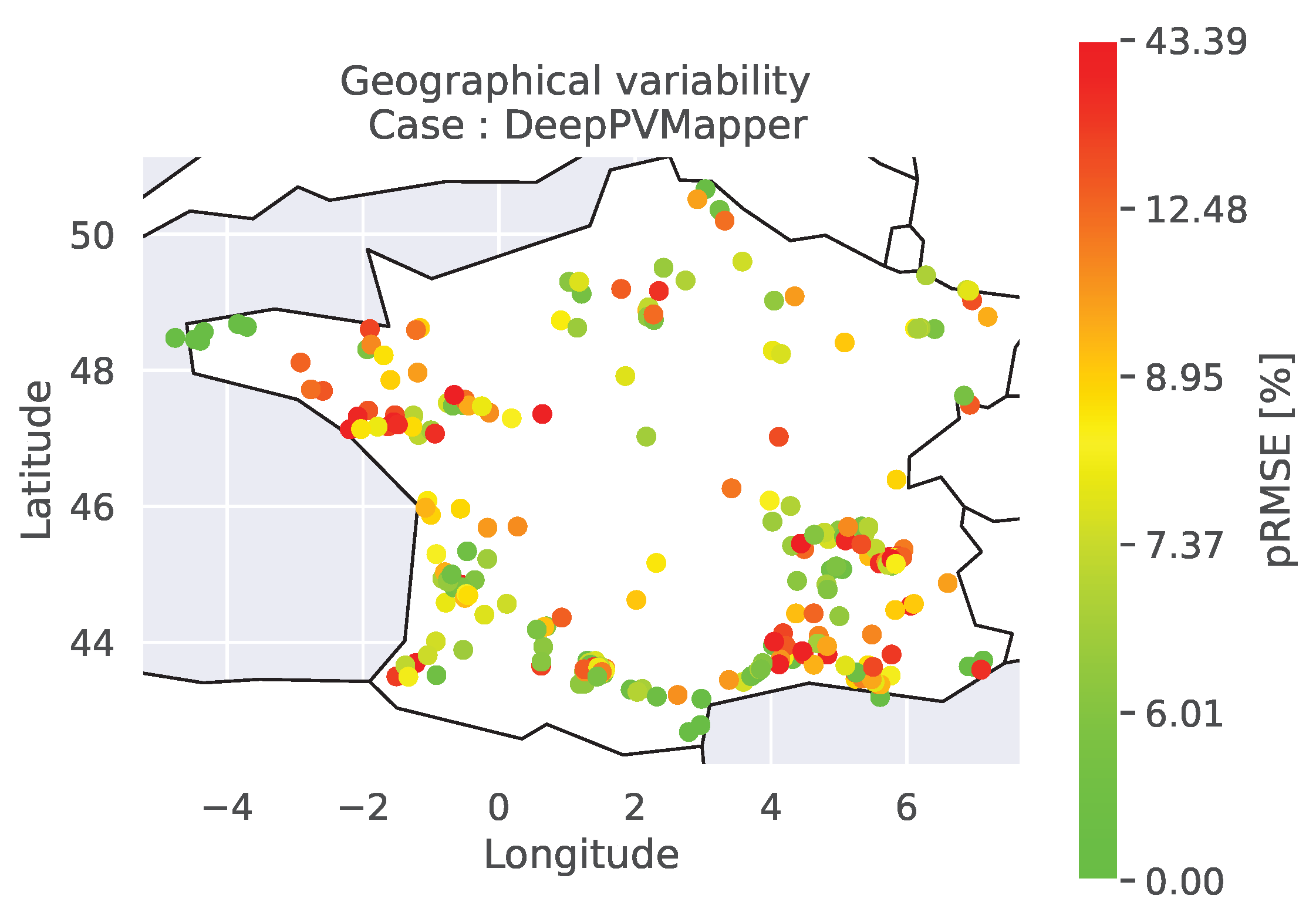
In addition to the quantitative evaluation, we qualitatively analyze the behavior of our PV power estimation model depending on the time of the day, the moment of the year, and the localization of the PV system.
Regarding the temporal analysis, we define time-of-the-day (TOD) timesteps or indices. TOD timesteps correspond to a 30-minute interval. The TOD timestep 0 corresponds to the time interval between 0h00 and 0h29, the timestep 1 corresponds to the time interval between 0h30 and 0h59, and the TOD timestep 47 to the time interval between 23h30 and 23h59. For each TOD timestep and each installation, we compute the pRMSE of the PV power estimation. We end up with a sample of errors for each TOD timestep, enabling us to compute relevant statistics (mean, median, interquantile ranges) regarding the evolution of the error in time. To measure the seasonality of the error, we filter the dates to keep only the Winter and Summer months. Summer months correspond to the months from June to September, and Winter months from December to March (4 months each).
4.2.2. Assessment of the Accuracy and Scalability of Our Proposed Approach
4.2.2.1. Comparison with the Oracle
The conversion model requires imputing a tilt and an azimuth angle and the installed capacity of the PV system. The conversion model is intended to work with parameters obtained from DeepPVMapper, and we refer to the conversion model parameterized with the system’s characteristics with these estimations as DeepPVMapper. Since we know from the BDPV database the true tilt and azimuth angles, we can compute an Oracle estimation, which reflects the best possible estimation to obtain given the conversion model and the weather data.
This comparison with the Oracle aims at assessing the accuracy of the estimation of the PV power production using parameters obtained using DeepPVMapper compared to the best possible accuracy that it is possible to attain with our conversion model and the weather data that we chose for this study, and which we considered as given.
4.2.2.2. Assessment of the Scalability: Behavior of the Error at the Aggregated Level
Our methodology estimates the PV power production at the individual installation level. In practice, the TSOs face hundreds of thousands of such systems. Therefore, evaluating how the estimation error behaves as the number of systems included in the study increases is necessary.
Our primary concern is that DeepPVMapper estimates the parameters of the PV system with a systematic bias (e.g., systematically underestimating the tilt angle or slightly shifting the azimuth angle). Should such cases occur, the estimation error at the aggregated level would no longer decrease with the number of installations, as the error terms at the individual installation level would no longer be independent [
24]. When considering the "bias," we focus on biases that could occur when aggregating the estimations, not biases at the individual installation level.
The sources of error identified and discussed by [
24] are the irradiation variability and the variability in plant characteristics. Relying on an estimation of the plant’s characteristics adds an additional source of variability, the variability in the
characterization error of the PV plants. This source of error should also be independent or negligible compared to the other (independent) sources of error if one wants the RMSE to converge toward the population mean.
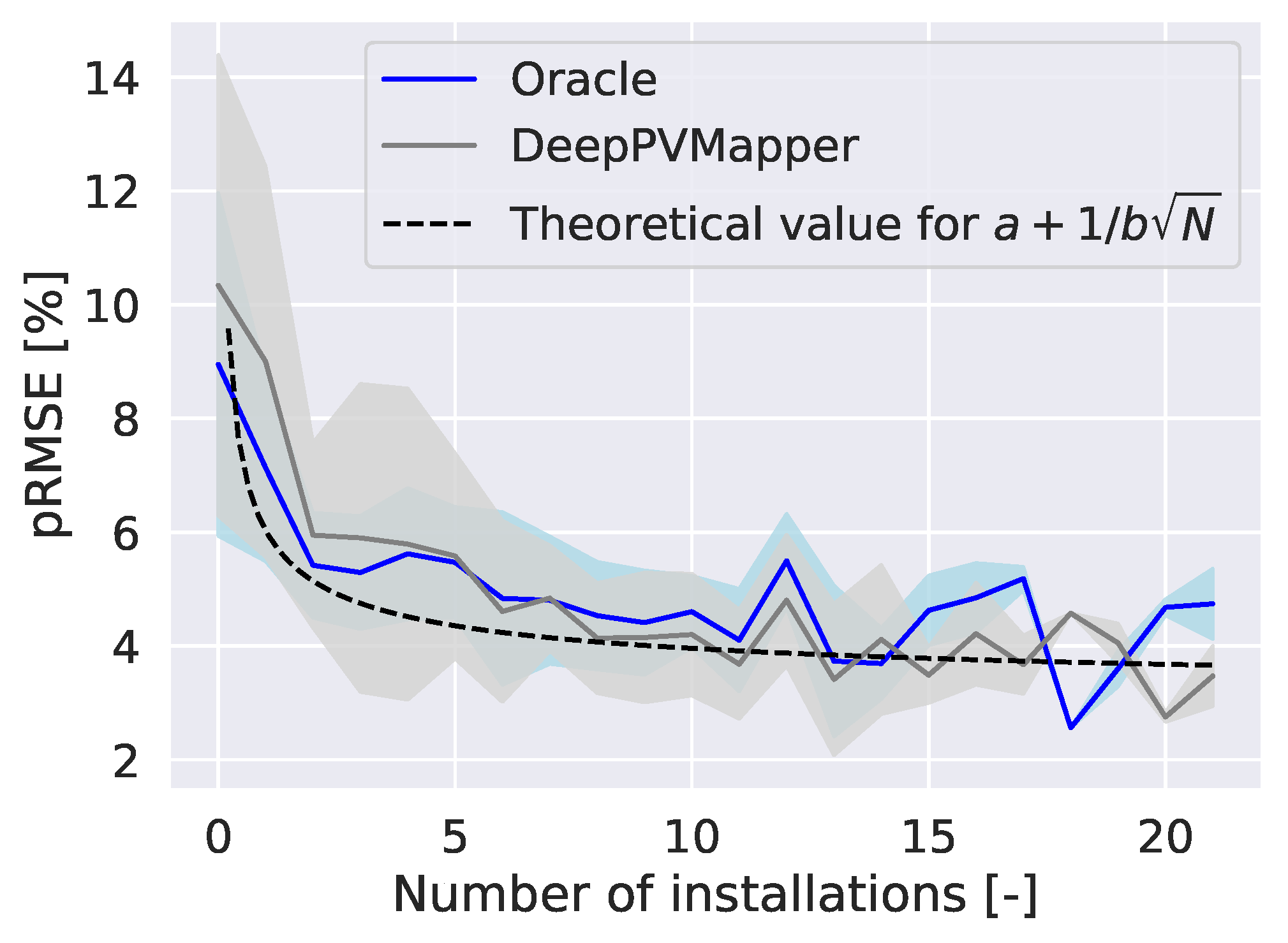
We empirically evaluate the behavior of the estimation error as the sample size increases by including an increasing number of installations in our sample and computing the error at the aggregated rather than individual installation level. We compare the behavior of the error with the PV system’s parameters estimated with DeepPVMapper and the behavior of the error of the Oracle.
5. Results
5.1. Our Approach Accurately Estimates the PV Power Production
Our main result, depicted in
Table 4, is that it is possible to improve rooftop PV observability by deriving rooftop PV power measurements at the installation scale using a simple conversion model, solar irradiance data, and limited information on the PV system. The estimation error, measured by the pRMSE, is about 10%. This approach does not require access to ground truth PV power measurements and can be used as a first guess to construct or reconstruct rooftop PV power measurements. In
Appendix C,
Table A1, we analyze the biases of our method and show that it exhibits a slight upward bias (in absolute terms) regarding the estimation of the PV power production.
5.2. Analysis of the Estimation Error
Temporal Trends
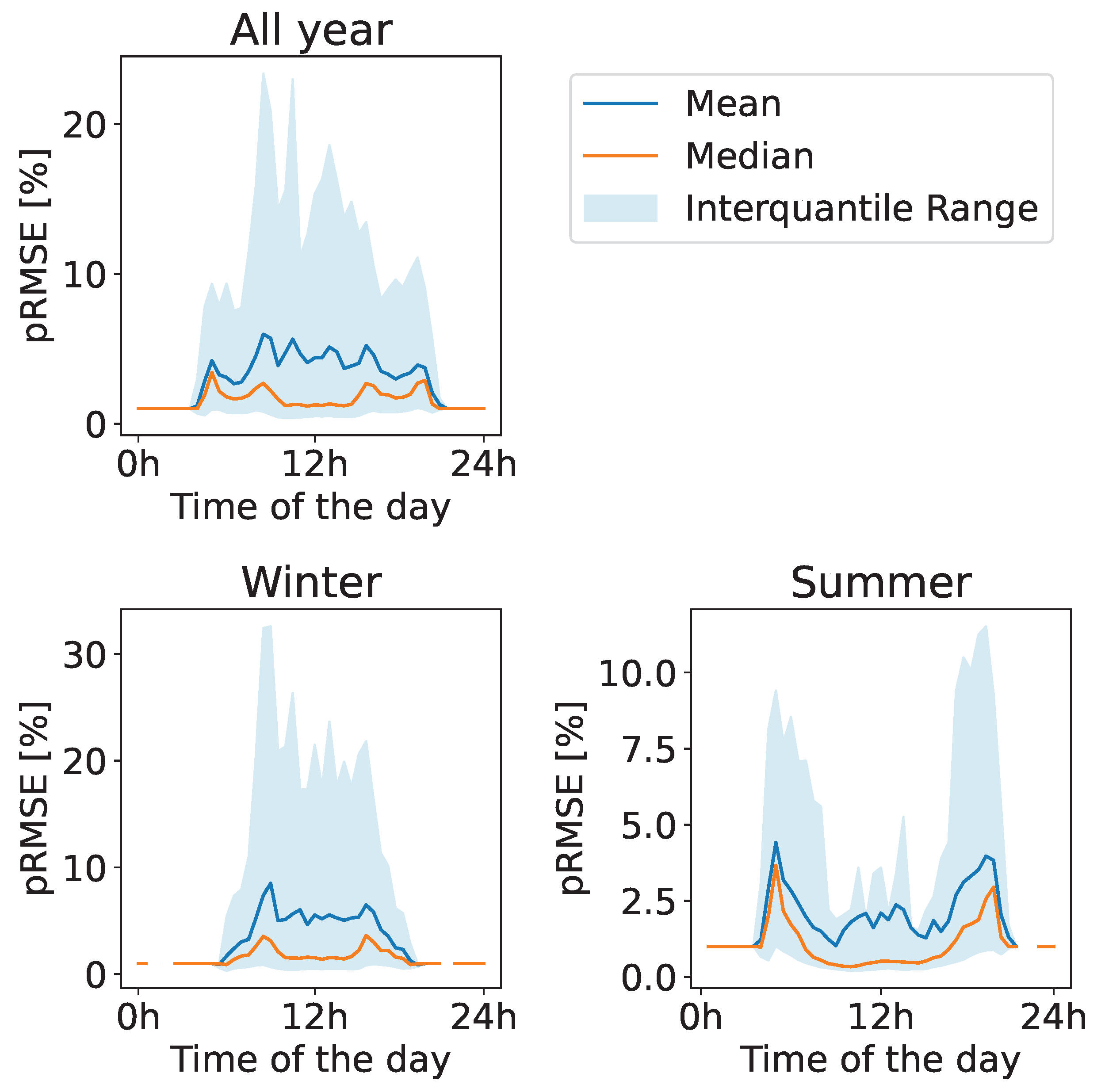
Figure 4 presents the analysis of the temporal variability of the error. The blue curve corresponds to the average error across the systems and estimations, and the orange curve corresponds to the median error. We also plot the interquantile ranges in light blue to highlight the dispersion of the errors as a function of the TOD timestep.
??, we show that results are qualitatively the same (with a lower error) when the conversion model is parameterized with the ground truth parameters.
On the "all year" chart, we only filter dates according to their hour of the day. We can see that the error is null during the night and increases to reach a peak during the day. The bottom charts show that the error variability is larger during winter and is high throughout the day. On the other hand, during summer, the error variability is high at dawn and dusk but decreases around noon. The higher uncertainty in the accuracy of our model during winter and summer dawn and dusk may be attributable to the fact that we do not take shadings into account. Indeed, [
54] reported a similar behavior with their model, which did not consider shadings. Another possible explanation is that our model neglects the self-consumption of power inverters and the behavior of the modules with low solar irradiance and high incidence angle. Finally, in winter, the higher uncertainty could also be caused by the greater difficulty in estimating the GHI [
55]. In
Appendix D, we further investigate the effect of the parameters on the temporal decomposition of the estimation error.
Spatial Trends
In
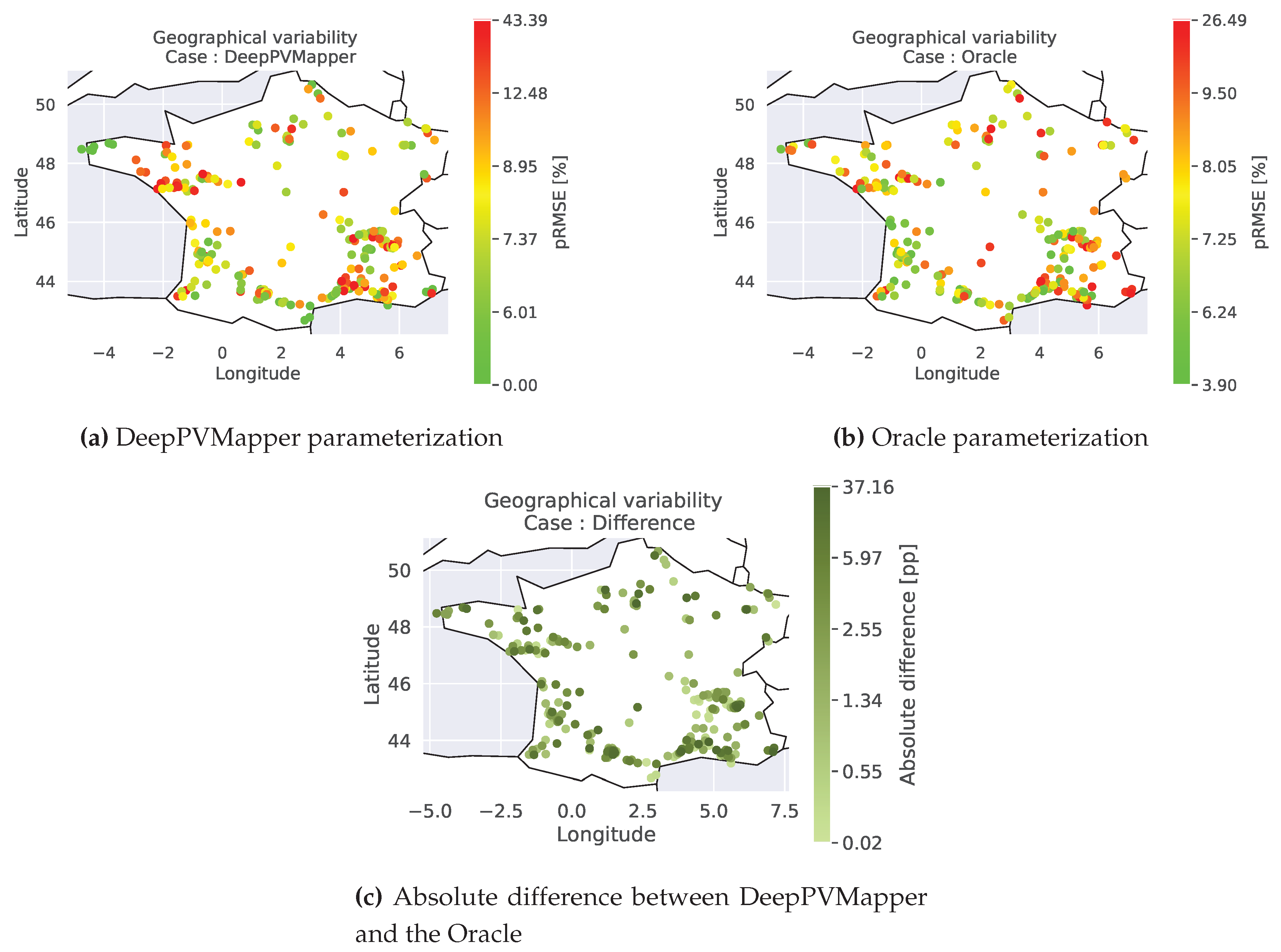
Figure 5, we investigate the geographical variability of the estimation error with the conversion model with the parameters obtained from DeepPVMapper. We find geographical clusters with larger estimation errors in France’s South East and the North West. This could be caused by the fact that the southeast of France is more hilly than western France so that shadings may be more critical. In
Appendix E, we compare the geographical distribution of the error with the Oracle parameterization and investigate the difference between the two, showing no evidence of systematic biases in the geographical distribution of the error of DeepPVMapper compared to the Oracle, reinforcing the conclusion that the geographical distribution of the error is mainly due to errors in the estimation of GHI.
5.3. Scalability of the Proposed Approach
Figure 6 shows the evolution of the estimation error as the number of considered installations increases. We can see that the error behavior when we input the PV system’s parameters from DeepPVMapper follows the same trend as that of the Oracle. We recall that the Oracle estimates PV power production using the parameters supplied by BDPV (i.e., the ground truth parameters on the PV system).
Figure 6 shows that our approach does not suffer from blatant biases that could threaten its ability to scale to thousands of systems.
6. Conclusion and Discussion
6.1. Conclusion
Transmission system operators (TSOs) lack accurate power measurements stemming from small-scale (less than or equal to 36 ) photovoltaic (PV) installations. In France, these installations represent 94% of the connected installations and 22% of the installed capacity. In the context of sustained growth of the overall installed capacity, ensuring the safe and optimal integration of rooftop PV into the grid is crucial to address the poor rooftop PV observability.
This work discusses whether rooftop PV observability can be improved by estimating the PV power production of rooftop PV systems at the individual scale using a physical-based conversion model, solar irradiance data, and rooftop PV characteristics estimated using remote sensing-based techniques.
Using ground truth power measurements of individual PV systems located over France, we show that such a method, which requires very little information on the PV systems, enables us to derive accurate estimations of the PV power production at the individual level.
We leverage a novel database of ground truth PV power measurements supplied by the non-profit association Asso BDPV to demonstrate that PV registry data can be efficiently combined with solar irradiance and temperature data through off-the-shelf conversion models to estimate the rooftop PV power production accurately. Our work shows that we can derive accurate estimations knowing only the PV system’s localization and installed capacity, reaching an estimation error (measured by the pRMSE) of about 10% of the nameplate capacity.
6.2. Limitations and Future Works
The main limitation of our work is that we could not analyze the behavior of our approach when aggregating hundreds of systems. Our analyses were limited to a few dozen systems. Therefore, we cannot correctly compare our approach with the TSO’s existing methods for estimating rooftop PV power production. As we lacked ground truth measurements to carry out such comparisons, we needed to either gather more data or make assumptions about constructing a PV power production reference.
More broadly, our framework focuses on the estimation of PV power curves at the individual installation level. Therefore, we do not consider the discrepancy between the estimated installed capacity and the actual installed capacity, resulting from detection errors of the algorithm used to construct the remote sensing-based registry.
Future works should further discuss the comparisons with the TSO’s current practice for estimating PV power production, both at the individual installation level and at the aggregated level. Besides, the benefits of more advanced conversion models could be discussed, e.g., considering shadings.
Author Contributions
Conceptualization, Gabriel Kasmi, Augustin Touron, Yves-Marie Saint-Drenan, Maxime Fortin and Laurent Dubus; Data curation, Yves-Marie Saint-Drenan; Formal analysis, Gabriel Kasmi; Funding acquisition, Laurent Dubus; Investigation, Gabriel Kasmi; Methodology, Gabriel Kasmi, Augustin Touron, Philippe Blanc, Yves-Marie Saint-Drenan, Maxime Fortin and Laurent Dubus; Project administration, Laurent Dubus; Software, Gabriel Kasmi; Supervision, Philippe Blanc, Yves-Marie Saint-Drenan and Laurent Dubus; Validation, Gabriel Kasmi and Augustin Touron; Writing – original draft, Gabriel Kasmi; Writing – review & editing, Gabriel Kasmi, Augustin Touron, Philippe Blanc, Yves-Marie Saint-Drenan, Maxime Fortin and Laurent Dubus. All authors have read and agreed to the published version of the manuscript.
Funding
This project is carried out as part of the Ph.D. thesis of Gabriel Kasmi, sponsored by the French transmission system operator RTE France and partly funded by the National Agency for Research and Technology (ANRT) under the CIFRE contract 2020/0685.
Acknowledgments
The authors gratefully acknowledge the support of RTE France and the ANRT for this project.
Appendix A Details on the Estimation of the PV Power Production Using PVWatts
Appendix A.1. Computation of the POA Irradiance
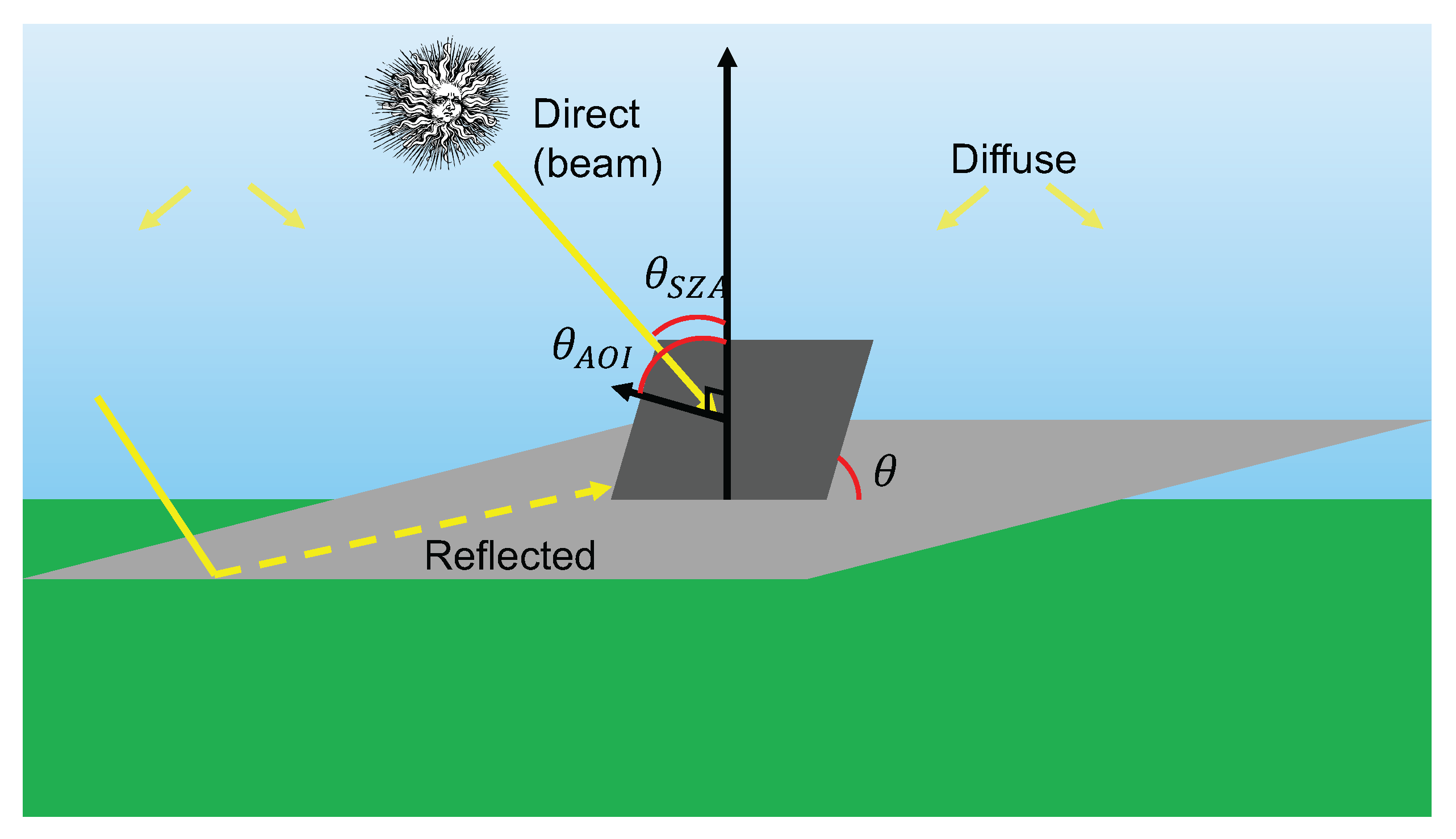
The POA irradiance corresponds to the solar irradiance incident on a surface that is adjusted to the tilt and azimuth angle of the array. It represents the solar energy reaching a surface considering its orientation towards the sun. The POA irradiance can be decomposed into three components:
A direct component (POA direct or beam irradiance): This is the solar radiation that reaches the surface in a direct line from the sun. It is the sunlight that travels directly through the atmosphere without being scattered or reflected,
A diffuse component (POA diffuse irradiance): This is the solar radiation that reaches the surface after being scattered by molecules and particles in the atmosphere. It includes the sunlight that comes from all directions other than the direct path from the sun,
A reflected component (reflected irradiance): The portion of sunlight that is reflected off nearby surfaces, such as the ground or surrounding structures, and reaches the surface of the PV module
The sum of these components gives the total POA irradiance. We leverage the Python library
pvlib [
56] to compute the POA irradiance. The function takes as input the solar zenith angle (SZA), the solar azimuthal angle, the top-of-atmosphere (TOA) sun position, the three components of solar radiation (GHI, DHI, and DNI), and the installation’s tilt and azimuth angles.
Appendix A.2. Computation of the Module Temperature
The performance of a PV module depends on its temperature and decreases when the temperature increases. We estimate the module temperature following [
57], given by equation (
A1):
In other words, the module temperature at time t corresponds to the sum of the atmospheric temperature at 2 meters, and the temperature increase due to the exposition of the module to the solar radiation. The temperature increase is weighted by the factor , meaning that we assume a linear relationship between the increase in temperature and the global POA (GPOA) irradiance at time t. denotes the irradiance under standard test conditions (STC) and is equal to 1000 .
Appendix A.3. Computation of the Effective POA Irradiance
The effective POA irradiance corresponds to the POA irradiance after accounting for the optical losses of the module. To account for these losses, we implement Martin and Ruiz’s IAM (incident angle modifier) model [
51,
52,
53]. This model returns incident angle modifiers (IAMs) applied to the POA irradiance to obtain the effective POA irradiance. Intuitively, this model accounts for the fact that the glass on the PV module reflects that the angular losses (AL) of PV modules are a function of the solar incident angle
[
51]. We considered reference values for a monocrystalline module.
where
is the weighted transmittance at incident angle
x,
the weighted reflectance at incident angle
x and
the "angular losses coefficient
, an empirical dimensionless parameter to fit in each case" [
51].
Then an angular factor
, corresponding to the IAM, is defined as the ratio between the module’s short circuit current
at indecent angle
to the
at normal incidence.
We compute the IAM for the three components of POA irradiance, and the effective POA is given by
Where
corresponds to the IAM,
the direct POA,
the diffuse POA component, and
the reflected POA component.
Figure A1 illustrates the different components of solar radiation considered to compute the effective plane-of-array incidence. "Direct," "Diffuse," and "Reflected" correspond to the components of solar radiation.
Figure A1.
Illustration of the POA irradiation modeled with our approach. indicates angles, "AOI": "angle of incidence" and "SZA": solar zenith angle. The light gray surface is flat, and the dark grey surface is tilted with tilt angle .
Figure A1.
Illustration of the POA irradiation modeled with our approach. indicates angles, "AOI": "angle of incidence" and "SZA": solar zenith angle. The light gray surface is flat, and the dark grey surface is tilted with tilt angle .
Appendix B Individual Installation Reports Used to Curate the Dataset
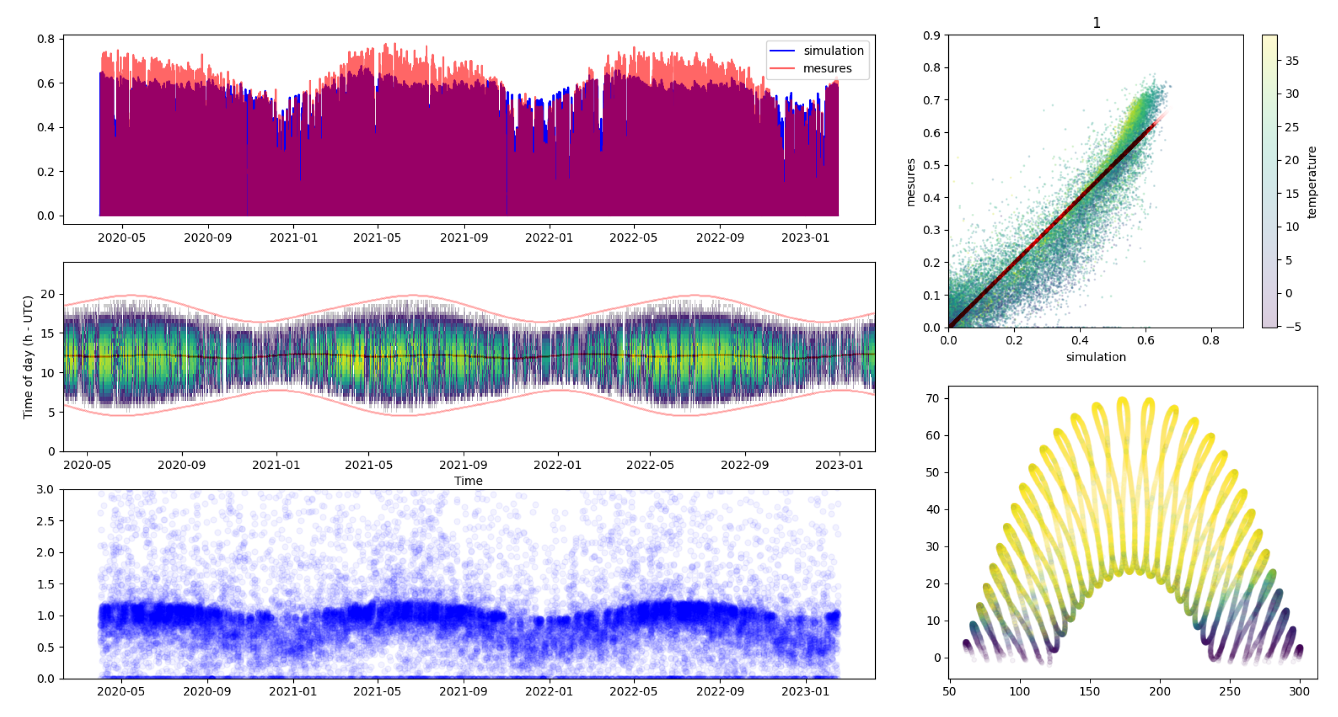
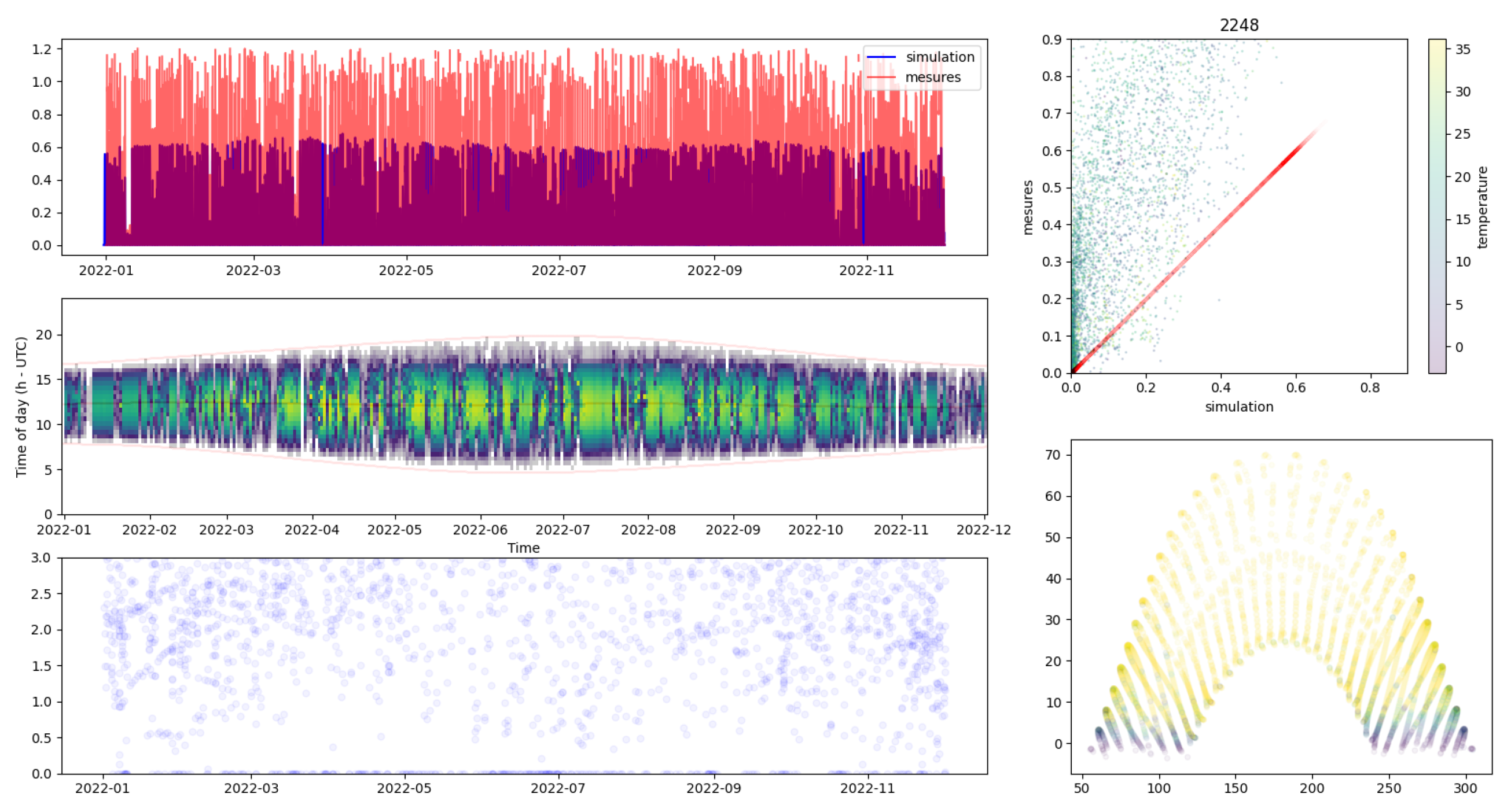
In addition to the quantitative inspections described in
Section 3.1.2, our quality check also relied on the qualitative examination of production reports such as those shown in
Figure A2 and
Figure A3. These reports consist in fitting a simulation model (different from our simple simulation model as the latter accommodates for all parameters of the PV installation) and comparing the production with the estimation.
Figure A2 and
Figure A3 present two systems that passed and failed our quality checks, respectively. We can see that in the case of installation # 2248, which failed the quality check, the estimation between the production and the estimation does not fit at all, indicating that either the localization of the installation is wrong (so the weather data is inaccurate) and that the installation does not work correctly as it produces much less than expected. We filtered out this installation because the different plots highlight diverging values between the estimation of the PV power production and the corresponding measurements.
Figure A2.
Example of an installation that passed the QC
Figure A2.
Example of an installation that passed the QC
Figure A3.
Example of an installation that failed the QC
Figure A3.
Example of an installation that failed the QC
Appendix C Bias Metrics of the Method for Estimating the PV Power Production
Table A1 presents the results of the estimation of the bias for the proposed method. We compute the bias according to four metrics: the mean bias deviation.
and the mean percentage error
, the mean absolute error
and the mean absolute percentage error
. Each metric is computed for one installation, and
Table A1 presents the mean and median over all the installations. We can see that the average error is quite high (first row of each case), but the median is much lower, indicating that overall, the method has few biases. Interestingly, the parameterization with DeepPVMapper seems to beat the Oracle according to the bias metrics.
Table A1.
Bias estimation metrics of the proposed estimation method for the parameterizations with the ground truth parameters ("Oracle") and the parameterization with the parameters estimated with DeepPVMapper ("DeepPVMapper").
Table A1.
Bias estimation metrics of the proposed estimation method for the parameterizations with the ground truth parameters ("Oracle") and the parameterization with the parameters estimated with DeepPVMapper ("DeepPVMapper").
| Case |
Mean bias deviation |
Mean absolute error |
Mean percentage error |
Mean absolute percentage error |
| |
[W] |
[W] |
[%] |
[%] |
| Oracle |
-73.64 |
137.03 |
-2.23 |
4.07 |
| |
-60.07 |
106.72 |
-2.02 |
3.67 |
| DeepPVMapper |
-26.39 |
158.72 |
-1.44 |
4.81 |
| |
-11.92 |
116.88 |
-0.43 |
4.04 |
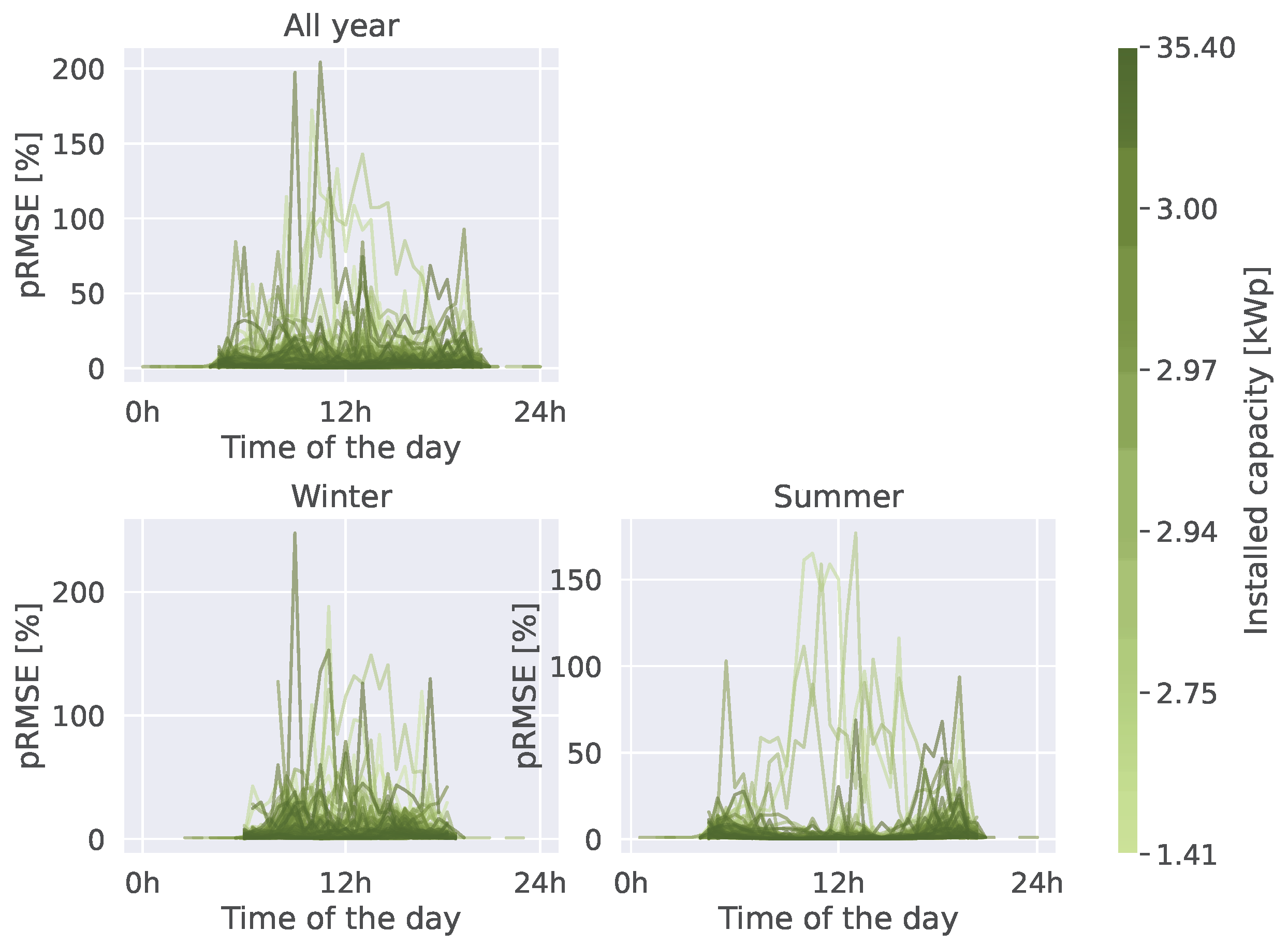
Appendix D Additional Trends on the Temporal Pattern of the Error
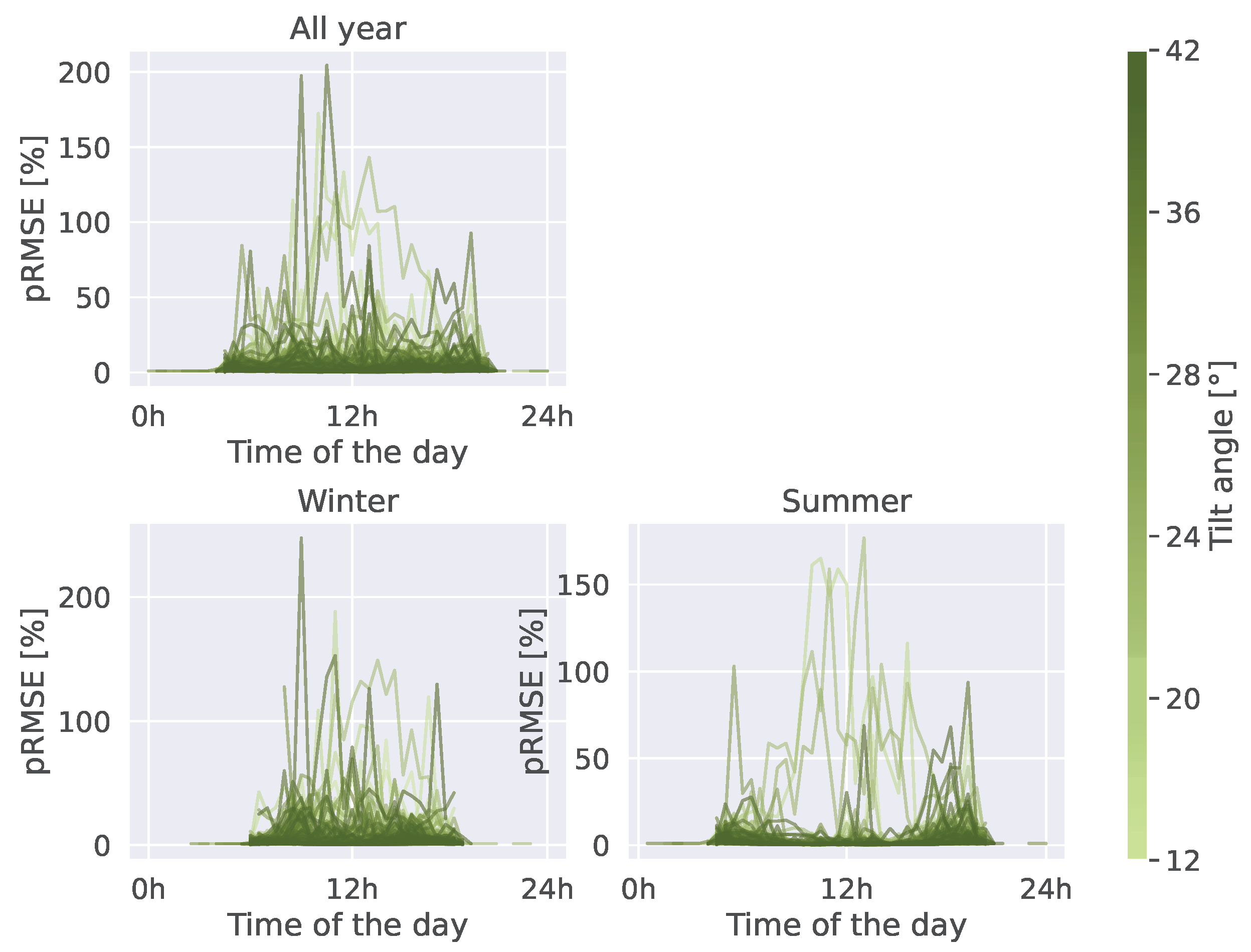
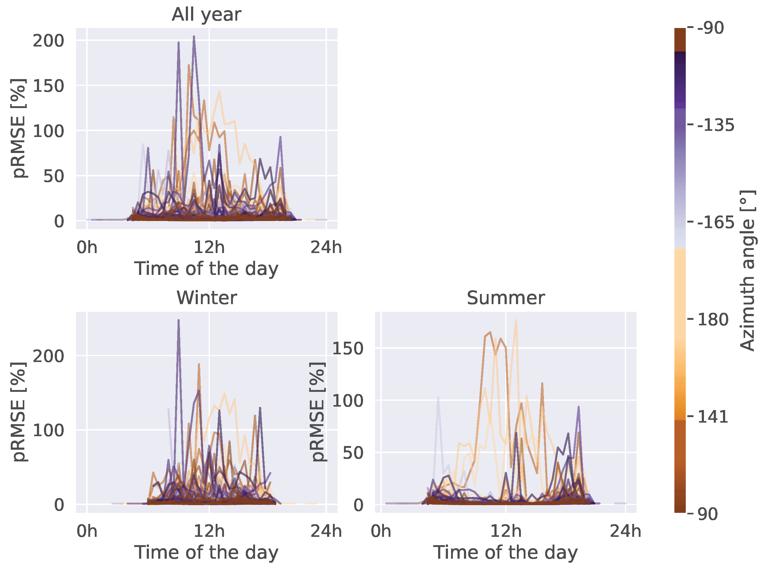
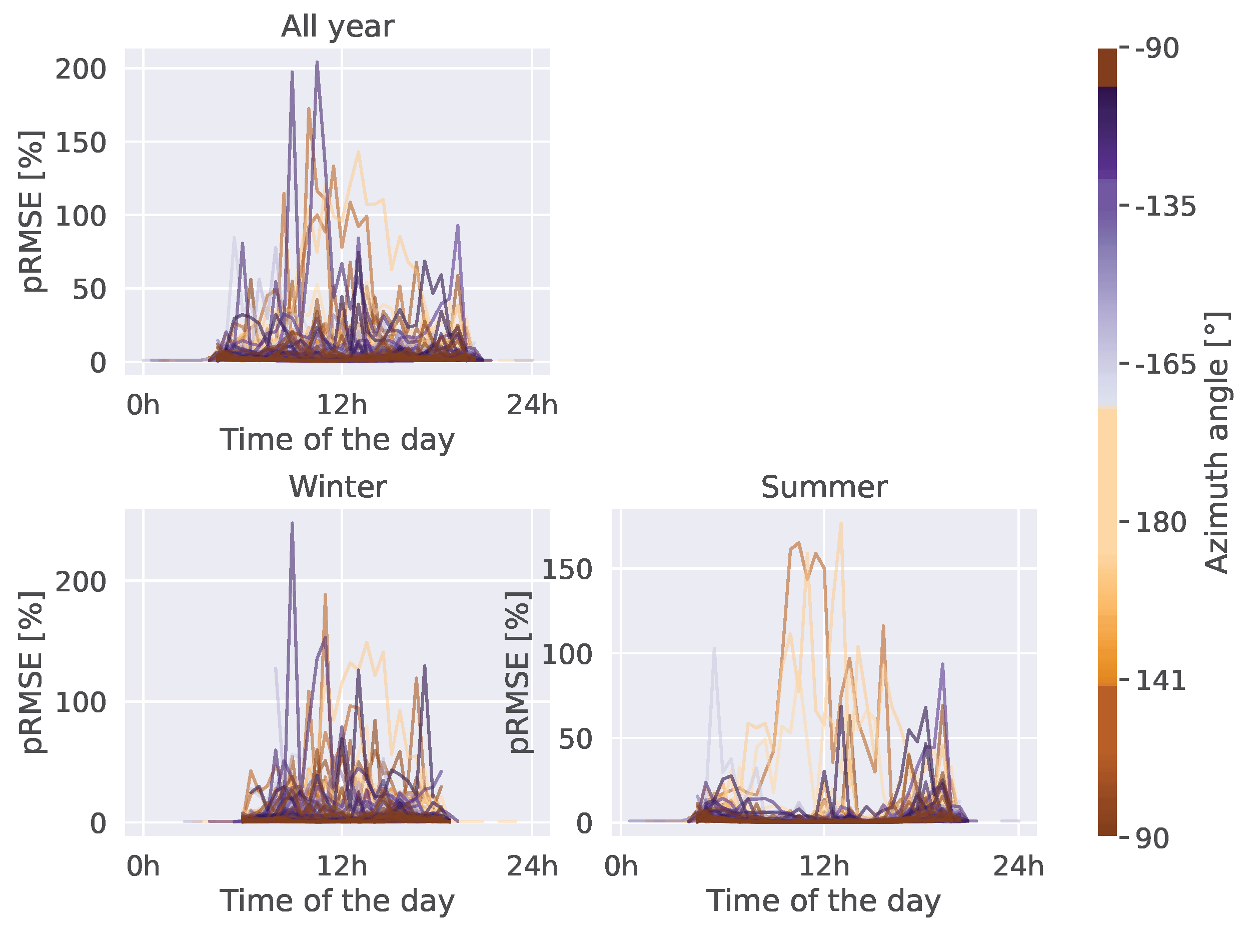
Figure A4,
Figure A5,
Figure A6 provide a decomposition of the temporal error depending on the installed capacity, tilt angle, and azimuth angle (respectively) of the system. We can see that the error is not correlated with any of those variables. On the other hand, we can see a couple of outliers for which the estimation error is very high. After further investigation, these installations corresponded to systems for which the ground truth location of the system was incorrect.
Figure A4.
Temporal variability of the estimation error depending on the installed capacity of the system..
Figure A4.
Temporal variability of the estimation error depending on the installed capacity of the system..
Figure A5.
Temporal variability of the estimation error depending on the tilt angle of the system..
Figure A5.
Temporal variability of the estimation error depending on the tilt angle of the system..
Figure A6.
Temporal variability of the estimation error depending on the azimuth angle of the system..
Figure A6.
Temporal variability of the estimation error depending on the azimuth angle of the system..
Figure A7.
Temporal variability of the estimation error depending on the azimuth angle of the system..
Figure A7.
Temporal variability of the estimation error depending on the azimuth angle of the system..
Figure A8 presents the temporal variability of the estimation error with a model parameterized with the ground truth parameters (i.e., the Oracle model). We can see that the patterns are the same as for DeepPVMapper. Only the average and maximum values for the error are lower.
Figure A8.
Temporal variability of the estimation error with a conversion model parameterized with the ground truth parameters (Oracle)..
Figure A8.
Temporal variability of the estimation error with a conversion model parameterized with the ground truth parameters (Oracle)..
Appendix E Additional Plots
Appendix E.1. Visualization of Generation Curves Generated with Our Conversion Model
Figure A9 depicts estimations of a generation curve using our conversion model. This small example illustrates that our estimation is well calibrated: the PV power production is well estimated, and there are no lags in the temporal variables.
Figure A9.
Power curves generated with our conversion model (orange) and comparison with ground truth data for a PV system located near Toulouse (France).
Figure A9.
Power curves generated with our conversion model (orange) and comparison with ground truth data for a PV system located near Toulouse (France).
Appendix E.2. Additional Plots on the Geographical Variability of the Estimation Error
Figure A10 depicts the geographical variability of the estimation error with the conversion model for two different parameterizations. Each point represents a PV system. The color indicates the error. The greener, the lower, and the redder, the higher the error. The error is measured using the pRMSE. We consider the parameters obtained from DeepPVMapper (
Figure A10a) and using the Oracle parameterization (
Figure A10b). As depicted in
Figure A10c, the difference between the errors between DeepPVMapper and the Oracle appears to be randomly distributed across France, showing no evidence of a systematic bias in the error of DeepPVMapper.
Figure A10.
Geographical variability of the estimation error with two parameterizations of the conversion model: DeepPVMapper (
Figure A10a) and the Oracle parameterization (
Figure A10b).
Figure A10c shows the absolute difference between DeepPVMapper and the Oracle.
Figure A10.
Geographical variability of the estimation error with two parameterizations of the conversion model: DeepPVMapper (
Figure A10a) and the Oracle parameterization (
Figure A10b).
Figure A10c shows the absolute difference between DeepPVMapper and the Oracle.
References
- Haegel, N.M.; Margolis, R.; Buonassisi, T.; Feldman, D.; Froitzheim, A.; Garabedian, R.; Green, M.; Glunz, S.; Henning, H.M.; Holder, B.; others. Terawatt-scale photovoltaics: Trajectories and challenges. Science 2017, 356, 141–143. Publisher: American Association for the Advancement of Science.
- IEA. Renewable Energy Statistics 2022. Technical report, IRENA, 2023.
- RTE France. Bilan électrique 2023, 2024.
- RTE France.; IEA. Conditions and Requirements for the Technical Feasibility of a Power System with a High Share of Renewables in France Towards 2050. Technical report, Paris, 2021.
- Pierro, M.; Liolli, F.R.; Gentili, D.; Petitta, M.; Perez, R.; Moser, D.; Cornaro, C. Impact of PV/Wind Forecast Accuracy and National Transmission Grid Reinforcement on the Italian Electric System. Energies 2022, 15, 9086. [Google Scholar] [CrossRef]
- Malof, J.M.; Rui, Hou.; Collins, L.M.; Bradbury, K.; Newell, R. Automatic solar photovoltaic panel detection in satellite imagery. 2015 International Conference on Renewable Energy Research and Applications (ICRERA); IEEE: Palermo, Italy, 2015; pp. 1428–1431. [Google Scholar] [CrossRef]
- Malof, J.M.; Li, B.; Huang, B.; Bradbury, K.; Stretslov, A. Mapping solar array location, size, and capacity using deep learning and overhead imagery, 2019.
- LeCun, Y.;Bengio,Y.;Hinton,G.Deeplearning. Nature 2015, 521, 436–444. Publisher: Nature Publishing Group. [CrossRef] [PubMed]
- Yu, J.; Wang, Z.; Majumdar, A.; Rajagopal, R. DeepSolar: A Machine Learning Framework to Efficiently Construct a Solar Deployment Database in the United States. Joule 2018, 2, 2605–2617. [Google Scholar] [CrossRef]
- Frimane, A.; Johansson, R.; Munkhammar, J.; Lingfors, D.; Lindahl, J. Identifying small decentralized solar systems in aerial images using deep learning. Solar Energy 2023, 262, 111822. [Google Scholar] [CrossRef]
- Lindahl, J.; Johansson, R.; Lingfors, D. Mapping of decentralised photovoltaic and solar thermal systems by remote sensing aerial imagery and deep machine learning for statistic generation. Energy and AI 2023, p. 100300. [CrossRef]
- Kasmi, G.; Dubus, L.; Saint-Drenan, Y.M.; Blanc, P. Towards Unsupervised Assessment with Open-Source Data of the Accuracy of Deep Learning-Based Distributed PV Mapping. Proceedings of MACLEAN: MAChine Learning for EArth ObservatioN Workshop co-located with the European Conference on Machine Learning and Principles and Practice of Knowledge Discovery in Databases (ECML/PKDD 2022), Grenoble, France, September 18-22, 2022; Corpetti, T.; Ienco, D.; Interdonato, R.; Pham, M.T.; Lefèvre, S., Eds. CEUR-WS.org, 2022, Vol. 3343, CEUR Workshop Proceedings.
- Mayer, K.; Rausch, B.; Arlt, M.L.; Gust, G.; Wang, Z.; Neumann, D.; Rajagopal, R. 3D-PV-Locator: Large-scale detection of rooftop-mounted photovoltaic systems in 3D. Applied Energy 2022, 310, 118469. [Google Scholar] [CrossRef]
- Freitas, S.;Silva, M.;Silva, E.;Marceddu, A.;Miccoli, M.;Gnatyuk, P.;Marangoni, L.;Amicone, A. AnArtificial Intelligence-Based Framework to Accelerate Data-Driven Policies to Promote Solar Photovoltaics in Lisbon. Solar RRL 2023, n/a, 2300597._eprint:https://onlinelibrary.wiley.com/doi/pdf/10.1002/solr.202300597. [CrossRef]
- Arnaudo, E.; Blanco, G.; Monti, A.; Bianco, G.; Monaco, C.; Pasquali, P.; Dominici, F. A Comparative Evaluation of Deep Learning Techniques for Photovoltaic Panel Detection from Aerial Images. IEEE Access 2023, pp. 1–1. [CrossRef]
- Lu, N.; Li, L.; Qin, J. PV Identifier: Extraction of small-scale distributed photovoltaics in complex environments from high spatial resolution remote sensing images. Applied Energy 2024, 365, 123311. [Google Scholar] [CrossRef]
- Yang, R.; He, G.; Yin, R.; Wang, G.; Zhang, Z.; Long, T.; Peng, Y. Weakly-semi supervised extraction of rooftop photovoltaics from high-resolution images based on segment anything model and class activation map. Applied Energy 2024, 361, 122964. [Google Scholar] [CrossRef]
- Saint-Drenan, Y.; Bofinger, S.; Fritz, R.; Vogt, S.; Good, G.; Dobschinski, J. An empirical approach to parameterizing photovoltaic plants for power forecasting and simulation. Solar Energy 2015, 120, 479–493. [Google Scholar] [CrossRef]
- Dobos, A. PVWatts Version 5 Manual. Technical Report NREL/TP-6A20-62641, 1158421, NREL, 2014. [CrossRef]
- Kasmi, G.; Dubus, L.; Saint-Drenan, Y.M.; Blanc, P. Assessment of the Reliablity of a Model’s Decision by Generalizing Attribution to the Wavelet Domain. XAI in Action: Past, Present, and Future Applications workshop at NeurIPS 2023. arXiv, 2023. arXiv:2305.14979 [cs, stat]. [CrossRef]
- RTE France. Energy Pathways to 2050. Technical report, RTE France, 2022.
- République française. Décret n° 2020-456 du 21 avril 2020 relatif à la programmation pluriannuelle de l’énergie, 2020.
- Lorenz, E.; Scheidsteger, T.; Hurka, J.; Heinemann, D.; Kurz, C. Regional PV power prediction for improved grid integration. Progress in Photovoltaics: Research and Applications 2011, 19, 757–771. [Google Scholar] [CrossRef]
- Saint-Drenan, Y.; Good, G.; Braun, M.; Freisinger, T. Analysis of the uncertainty in the estimates of regional PV power generation evaluated with the upscaling method. Solar Energy 2016, 135, 536–550. [Google Scholar] [CrossRef]
- Puttemans, S.; Ranst, W.V.; Goedemé, T. Detecting of photovoltaic installations in RGB aerial imaging: a comparative study. Proceedings of GEOBIA 2016 : Solutions and synergies, 14-16 September 2016, Enschede, Netherlands. University of Twente, Faculty of Geo-Information Science and Earth Observation (ITC), 2016. [CrossRef]
- de Hoog, J.; Maetschke, S.; Ilfrich, P.; Kolluri, R.R. Using Satellite and Aerial Imagery for Identification of Solar PV: State of the Art and Research Opportunities. Proceedings of the Eleventh ACM International Conference on Future Energy Systems; ACM: Virtual Event Australia, 2020; pp. 308–313. [CrossRef]
- Bradbury, K.; Saboo, R.; L Johnson, T.; Malof, J.M.; Devarajan, A.; Zhang, W.; M Collins, L.; G Newell, R. Distributed solar photovoltaic array location and extent dataset for remote sensing object identification. Scientific data 2016, 3, 1–9. Publisher: Nature Publishing Group.
- Malof, J.M.; Bradbury, K.; Collins, L.M.; Newell, R.G. Automatic detection of solar photovoltaic arrays in high resolution aerial imagery. Applied Energy 2016, 183, 229–240. [Google Scholar] [CrossRef]
- Malof, J.M.; Collins, L.M.; Bradbury, K.; Newell, R.G. A deep convolutional neural network and a random forest classifier for solar photovoltaic array detection in aerial imagery. 2016 IEEE International Conference on Renewable Energy Research and Applications (ICRERA). IEEE, 2016, pp. 650–654.
- Li, Q.; Feng, Y.; Leng, Y.; Chen, D. SolarFinder: Automatic Detection of Solar Photovoltaic Arrays. 2020 19th ACM/IEEE International Conference on Information Processing in Sensor Networks (IPSN); IEEE: Sydney, NSW, Australia, 2020; pp. 193–204. [Google Scholar] [CrossRef]
- Wang, M.; Cui, Q.; Sun, Y.; Wang, Q. Photovoltaic panel extraction from very high-resolution aerial imagery using region–line primitive association analysis and template matching. ISPRS Journal of Photogrammetry and Remote Sensing 2018, 141, 100–111. [Google Scholar] [CrossRef]
- Devarajan, A.; Kellish, B.; Kido, C.; Newman, A.; Bradbury, K. Automated Rooftop Solar PV Detection and Power Estimation through Remote Sensing, 2016.
- Golovko, V.; Bezobrazov, S.; Kroshchanka, A.; Sachenko, A.; Komar, M.; Karachka, A. Convolutional neural network based solar photovoltaic panel detection in satellite photos. 2017 9th IEEE International Conference on Intelligent Data Acquisition and Advanced Computing Systems: Technology and Applications (IDAACS); IEEE: Bucharest, 2017; pp. 14–19. [Google Scholar] [CrossRef]
- Golovko, V.; Kroshchanka, A.; Bezobrazov, S.; Sachenko, A.; Komar, M.; Novosad, O. Development of Solar Panels Detector. 2018 International Scientific-Practical Conference Problems of Infocommunications. Science and Technology (PIC S&T); IEEE: Kharkiv, Ukraine, 2018; pp. 761–764. [CrossRef]
- Yuan, J.; Yang, H.H.L.; Omitaomu, O.A.; Bhaduri, B.L. Large-scale solar panel mapping from aerial images using deep convolutional networks. 2016 IEEE International Conference on Big Data (Big Data); IEEE: Washington DC, USA, 2016; pp. 2703–2708. [Google Scholar] [CrossRef]
- Huang, B.; Collins, L.M.; Bradbury, K.; Malof, J.M. Deep Convolutional Segmentation of Remote Sensing Imagery: A Simple and Efficient Alternative to Stitching Output Labels. IGARSS 2018 - 2018 IEEE International Geoscience and Remote Sensing Symposium; IEEE: Valencia, 2018; pp. 6899–6902. [Google Scholar]
- Camilo, J.; Wang, R.; Collins, L.M.; Bradbury, K.; Malof, J.M. Application of a semantic segmentation convolutional neural network for accurate automatic detection and mapping of solar photovoltaic arrays in aerial imagery, 2018. arXiv:1801.04018.
- Kausika, B.B.; Nijmeijer, D.; Reimerink, I.; Brouwer, P.; Liem, V. GeoAI for detection of solar photovoltaic installations in the Netherlands. Energy and AI 2021, 6, 100111. [Google Scholar] [CrossRef]
- Mayer, K.; Wang, Z.; Arlt, M.L.; Neumann, D.; Rajagopal, R. DeepSolar for Germany: A deep learning framework for PV system mapping from aerial imagery. 2020 International Conference on Smart Energy Systems and Technologies (SEST); IEEE: Istanbul, Turkey, 2020; pp. 1–6. [Google Scholar] [CrossRef]
- Kasmi, G.; Laurent, D.; Philippe, B.; Saint-Drenan, Y.M. DeepPVMapper, 2023. [CrossRef]
- Rausch, B.; Mayer, K.; Arlt, M.L.; Gust, G.; Staudt, P.; Weinhardt, C.; Neumann, D.; Rajagopal, R. An Enriched Automated PV Registry: Combining Image Recognition and 3D Building Data. NeurIPS 2020 Workshop on Tackling Climate Change with Machine Learning, 2020.
- Trémenbert, Y.; Kasmi, G.; Dubus, L.; Saint-Drenan, Y.M.; Blanc, P. PyPVRoof: a Python package for extracting the characteristics of rooftop PV installations using remote sensing data, 2023. arXiv:2309.07143.
- de Hoog, J.; Perera, M.; Bandara, K.; Senanayake, D.; Halgamuge, S. Solar PV Maps for Estimation and Forecasting of Distributed Solar Generation. ICML 2021 Workshop on Tackling Climate Change with Machine Learning, 2021.
- Perera, M.; De Hoog, J.; Bandara, K.; Halgamuge, S. Multi-resolution, multi-horizon distributed solar PV power forecasting with forecast combinations. Expert Systems with Applications 2022, 205, 117690. [Google Scholar] [CrossRef]
- Pecan Street. Dataport – Pecan Street Inc., 2024.
- Walch, A.; Rüdisüli, M.; Castello, R.; Scartezzini, J.L. Quantification of existing rooftop PV hourly generation capacity and validation against measurement data. Journal of Physics: Conference Series 2021, 2042, 012011. [Google Scholar] [CrossRef]
- Kasmi, G.; Saint-Drenan, Y.M.; Trebosc, D.; Jolivet, R.; Leloux, J.; Sarr, B.; Dubus, L. A crowdsourced dataset of aerial images with annotated solar photovoltaic arrays and installation metadata. Scientific Data 2023, 10, 59. [Google Scholar] [CrossRef] [PubMed]
- BDPV. Rapport d’analyse de votre installation photovoltaïque - Information - BDPV, 2024.
- Qu, Z.; Oumbe, A.; Blanc, P.; Espinar, B.; Gesell, G.; Gschwind, B.; Klüser, L.; Lefèvre, M.; Saboret, L.; Schroedter-Homscheidt, M.; Wald, L. Fast radiative transfer parameterisation for assessing the surface solar irradiance: The Heliosat-4 method. Meteorologische Zeitschrift 2017, 26, 33–57. [Google Scholar] [CrossRef]
- Hersbach, H.; Bell, B.; Berrisford, P.; Hirahara, S.; Horányi, A.; Muñoz-Sabater, J.; Nicolas, J.; Peubey, C.; Radu, R.; Schepers, D.; Simmons, A.; Soci, C.; Abdalla, S.; Abellan, X.; Balsamo, G.; Bechtold, P.; Biavati, G.; Bidlot, J.; Bonavita, M.; De Chiara, G.; Dahlgren, P.; Dee, D.; Diamantakis, M.; Dragani, R.; Flemming, J.; Forbes, R.; Fuentes, M.; Geer, A.; Haimberger, L.; Healy, S.; Hogan, R.J.; Hólm, E.; Janisková, M.; Keeley, S.; Laloyaux, P.; Lopez, P.; Lupu, C.; Radnoti, G.; de Rosnay, P.; Rozum, I.; Vamborg, F.; Villaume, S.; Thépaut, J.N. The ERA5 global reanalysis. Quarterly Journal of the Royal Meteorological Society 2020, 146, 1999–2049. _eprint: https://onlinelibrary.wiley.com/doi/pdf/10.1002/qj.3803. [CrossRef]
- Martin, N.; Ruiz, J.M. Calculation of the PV modules angular losses under field conditions by means of an analytical model. Solar Energy Materials and Solar Cells 2001, 70, 25–38. [Google Scholar] [CrossRef]
- Martín, N.; Ruiz, J.M. A new model for PV modules angular losses under field conditions. International Journal of Solar Energy 2002, 22, 19–31. Publisher: Taylor & Francis _eprint: https://doi.org/10.1080/01425910212852. [CrossRef]
- Martín, N.; Ruiz, J.M. Annual angular reflection losses in PV modules. Progress in Photovoltaics: Research and Applications 2005, 13, 75–84. _eprint: https://onlinelibrary.wiley.com/doi/pdf/10.1002/pip.585. [CrossRef]
- Walch, A.; Castello, R.; Mohajeri, N.; Scartezzini, J.L. Big data mining for the estimation of hourly rooftop photovoltaic potential and its uncertainty. Applied Energy 2020, 262, 114404. Publisher: Elsevier.
- Lopes, F.M.; Silva, H.G.; Salgado, R.; Cavaco, A.; Canhoto, P.; Collares-Pereira, M. Short-term forecasts of GHI and DNI for solar energy systems operation: assessment of the ECMWF integrated forecasting system in southern Portugal. Solar Energy 2018, 170, 14–30. [Google Scholar] [CrossRef]
- Holmgren, W.; Hansen, C.; Mikofski, M. pvlib python: a python package for modeling solar energy systems. Journal of Open Source Software 2018, 3, 884. [Google Scholar] [CrossRef]
- Ross Jr, R. Design Techniques for Flat-Plate Photovoltaic Arrays. 15th Photovoltaic Specialists Conference;, 1981; pp. 1126–1132.
| 1 |
In this article, we refer to as "rooftop" PV installations installations with an installed capacity lower than 36 . We may also refer to these installations as small-scale or distributed. |
| 2 |
The PPE (multiannual energy planning) is the French legislative framework that defines energy consumption and generation goals. |
| 3 |
Orthoimages are aerial or satellite images whose geometry has been rectified so that each point can be superimposed on a corresponding planar map. In other words, an orthophotograph appears to be taken at the vertical of all the points it features, these points being located on perfectly flat terrain |
| 4 |
The F1-score measures the performance of a binary classifier. A perfect classifier has a score of 1. It corresponds to the harmonic mean between a classifier’s precision (correct detections among all detections) and recall (correct detections among all targets). |
| 5 |
The metric used by [ 9] is the mean relative error (MRE), defined as follows:
|
|
Disclaimer/Publisher’s Note: The statements, opinions and data contained in all publications are solely those of the individual author(s) and contributor(s) and not of MDPI and/or the editor(s). MDPI and/or the editor(s) disclaim responsibility for any injury to people or property resulting from any ideas, methods, instructions or products referred to in the content. |
© 2024 by the authors. Licensee MDPI, Basel, Switzerland. This article is an open access article distributed under the terms and conditions of the Creative Commons Attribution (CC BY) license (http://creativecommons.org/licenses/by/4.0/).
