Preprint
Review

Uncertainties in Plant Species Niche Modelling Under Climate Change Scenarios

Altmetrics

Downloads

141

Views

46

Comments

0

A peer-reviewed article of this preprint also exists.

Submitted:

12 July 2024

Posted:

15 July 2024

You are already at the latest version

Alerts
Abstract
Species distribution models (SDMs) are usually used to predict current species’ geographic distributions and to forecast the impact of climate change, with different aims, such as conservation, and biodiversity management. SDMs use has been increasing in the last decades, however, they are vulnerable to parametrization and data quality input. Thus, inappropriate input can lead to potential unreliability in results. In this context, the most used data and methodologies in SDM, and putative deviations from the consensual best practices, were identified, by analysing recent literature (2018 to 2022). Results show that the parameters presented more consistently are the chosen algorithm (MaxEnt was used in 98% of the studies), the accuracy measures, and the time windows. Many papers fail to specify other parameters, limiting the reproducibility of the studies. Some papers also fail to provide information about the target species: only a fraction of the species' range is considered, or no justification for including specific variables in the model is provided. These options can decrease reliability in predictions under future scenarios since data provided to the model is inaccurate from the start or there is insufficient information for outputs discussion.
Keywords: 
Subject: Environmental and Earth Sciences  -   Ecology

1. Introduction

The need for spatial explicit results when assessing climate change impacts on species distribution promoted the search for a deep understanding about abiotic factors influence on species distribution patterns. A task facilitated by the increasing availability of environmental and species occurrence data with high resolution, namely for climatic scenarios, and dedicated tools, such as species distribution modelling techniques based on a wide array of algorithms based on correlation [1,2].
Species distribution models (SDMs) are widely used to predict species ranges and environmental niches, and their use has been increasing over the last two decades [1]. Models of correlative nature are more common, since they relate species occurrence data and environmental variables, generating maps predicting past, present or future species distributions [2,3,4].
The SDMs have been used for species conservation purposes and biodiversity management, like selecting locations for protected areas, habitat restoration actions, and/or species translocation, especially in the context of global climate change [5,6,7,8,9,10,11,12]. Under climate change scenarios, such an approach was used to assess possible impacts on biodiversity [12,13], aiming to assess potential changes in species suitable areas, from expansion [14,15] to contraction [16,17,18,19], and sometimes even extinction [20,21].
The choices made during the modelling process can significantly affect model predictive performance, and predictive results may vary greatly due to those choices [1,22,23], so models must be fitted for the purpose, and options should be carefully considered [12]. Possible inaccuracies or uncertainties sources can arise in different steps [24,25,26,27]. These sources may include data source - occurrences, environmental data – including future climate change scenarios; spatial niche truncation - use of a fraction of geographical and ecological range; campling effect - new conditions outside the range used to calibrate models; parametrization in the modelling process - variable selection and variable correlation; using only climatic variables; evaluation strategies; limited models discussion. Several authors have already looked into these issues, addressing different errors that can lead to inaccurate results [2,28,29,30,31,32,33,34,35,36,37,38,39].
Unreliable species' occurrence data can lead to models that underestimate suitable areas [34], affecting the quality of performed models [5]. Data sources for SDM can be collected from various sources, such as museums or other natural history collections, bibliographies, field surveys and databases. Data coming exclusively from museums or other natural history collections can be incomplete or biased, concerning the actual range of the species, since they were probably collected in more accessible locations [24]. Otherwise, collecting data from systematic field surveys can lead to some areas oversampling, compared to others [31]. Ideally, systematic surveys should be performed in the species total range area [5]. These surveys can be feasible for species with small range sizes, but highly demanding for species with wide ranges [36,40]. Online platforms (e.g. GBIF) currently provide occurrence data commonly used to estimate climate change impacts on species distributions. However, differences in funding between nations and data sharing lead to differences in contribution, creating spatial bias due to uneven effort [28,34]. Also, data collected by the general public may have several errors, such as misidentification and georeferencing errors or sampling bias across more accessible areas, near cities and roads [41], data storage and mobilization [28,34].
Future climate scenarios are based on emissions and development scenarios, established by the Intergovernmental Panel on Climate Change (IPCC). The more recent were released in their Assessment Report (AR6) [42]. These scenarios are projected based on possible development scenarios which consider different levels of greenhouse gas emissions, population growth, economic and technological development, and land use [43,44,45,46,47]. Although these scenarios are now robust projections and essential in climate change research and assessment [45], they are still scenarios and may be prone to errors and uncertainties, as well as the models based on them [29,48,49].
Study area limits are critical when modelling species suitability. When data from a restricted area of the species is used not all the abiotic conditions endured by the species may be considered, compromising the models' ability to capture the full range of suitable areas [2,50]. Leaving out marginal areas and marginal populations may also compromise results, since those populations may be adapted to more extreme conditions [51,52]. In these situations, called spatial niche truncation, only a subset of species ecological niche is considered so it can lead to incorrect forecasts when projecting future suitability [53,54]. Species occurrence data should be as comprehensive as possible to improve SDM results and represent environments and geographical areas where the species can live and disperse [5]. In fact, in studies that assess climate change effects, it might be critical to consider areas beyond the species' present range, accounting for locations that may reflect potential future environmental conditions [55]. Models cannot account for unknown conditions and assess their suitability in the future, thus, it is essential to include areas with conditions that do not yet exist in our study area which might be present in the future [32,33,39,52,55].
Climate variables greatly influence plant species' spatial (and temporal) distribution. However, these are not the only variables that explain their distribution, especially when dealing with restricted areas and high-resolution data. Other environmental and abiotic variables (e.g., soil, topography, fire) are also important when modelling distributions and range shifts [35,38,56,57], and the rejection of non-climatic environmental variables must be based on variable selection methods. The inclusion of such variables might also support the identification of other restrictive factors, namely associated with land use, since areas with greater slopes present lower human pressure [38] and register a higher number of occurrences, or might act as limiting factor themselves, like soil conditions, once it is unlikely that the species will be able to establish itself on unsuitable soil conditions even under appropriate climatic conditions [56,57,58,59]. So, the exclusive use of climate data can erroneously estimate a species' range, often producing overpredictions [57]. However, not all available variables should be blindly included in the model since these variables may be highly correlated [60,61], sharing high amounts of information [30]. In this case, variables with indirect effects (e.g. altitude) should be discarded, and correlated variables with direct influence (temperature or precipitation) [62,63]should remain, namely those with high biological significance for the species under analysis, contributing to i) simplify the interpretation of the model [64], ii) avoid over-fitted results, and iii) eliminate crossed effects on the response curves of each variable, once inaccuracies caused by interactions with other variables will remain when correlated variables are in use [2,65], becoming difficult to disentangle the influence of each variable [60]. This might be a severe drawback when a model is fitted on data from one area or time and projected to another area or period with a different or unknown structure of collinearity since collinearity between environmental variables is not constant in space and time [30]. It is impossible to eliminate collinearity, but it can be reduced [30]. There are several methods to quantify collinearity. One of the most effective is to select variables using a threshold under a specific value of correlation coefficients (e.g., |r| <0.7) [30,60]. Ignoring environmental variables that are determinant to tackle the species' ecology can lead to unlikely predictions of species responses to climate change (Guevara et al., 2018). Therefore, it is crucial to know the species' ecological preferences, to select the most meaningful variables to include in the model and to perform a model as reliably as possible [24,30,60,66,67].
There are many techniques and modelling algorithms available to perform SDMs, which belong to different categories of models, such as regression methods – generalized linear models (GLM), generalized additive model (GAM) and multivariate adaptive regression spline (MARS); classification methods – classification tree analysis (CTA) and Flexible Discriminant Analysis (FDA); machine learning algorithms – random forest (RF), Boosted Regression Tree (BRT) and Maximum Entropy (MaxEnt); [37,68,69], and others – Support Vector Machine (SVM) [70]. No single model is superior in all situations [70,71], so the algorithm's choice depends on the data specificities and the study objective [72].
Evaluation strategies or performance metrics are important to assess the discriminatory capacity of a model, or its ability to distinguish suitable from unsuitable conditions. There are several ways to assess model performance, such as sensitivity (the proportion of presences correctly predicted); specificity (the proportion of absences correctly identified); Cohen's Kappa Statistic (kappa); true skill statistic (TSS); percentage of correct classification rate (CCR); Area Under the ROC Curve (AUC); and error rate (ER) [22,73]. The most widely used evaluation metrics are AUC and TSS [2,74], but even the most widely used performance metrics have important limitations for ecological studies [74,75,76]. They are designed to reflect the trade-off between sensitivity and specificity and generally weigh sensitivity and specificity equally [77]. The single-use of AUC can identify well-fitting and strongly predictive over-fitted models [48]. The AUC value depends on the size of the study area: if the area is large enough to comprehend different habitats from those occupied by the species, the AUC will be higher, even if the model is not that good, since more points with correct predictions of low suitability are considered [75,77]. The same occurs with the TSS, which tends to be correlated with the AUC. Also, TSS depends on species prevalence and may lead to misleading results [78].
These common and recurrent mistakes during SDM application have led to the publication of several works that intend to standardize SDM procedures, improving their quality and reproducibility [5,6,12,64,79].
In this context, the main objective of this study is to analyze the available literature dedicated to assessing climate change effects on plant distribution, based on niche modelling, to understand:
  • what are the most used data and methodologies in recent papers, namely those related to model calibration;
  • what are the most common deviations from consensual best practices and what information is most omitted from methodological descriptions;
  • identify how far the faults referred to above are identified and discussed;
  • identify new recommendations to improve SDM results, making them clearer and more comprehensive.
The analysis considers the methodologies used in recent papers, from species occurrence data to abiotic variables data sources, and its implications in models' accuracy and potential reproduction by pairs. Key aspects of the SDM elements were registered for each paper and assembled into a database, i) the source of species occurrence data, ii) the area analyzed, iii) the type of data (presence only, pseudo-absence, absence data), iv) the abiotic variables, v) the variables' selection, vi) the used algorithm (s) for modelling, vii) the model performance metrics, viii) the use of an ensemble model, ix) the climate scenario studied, x) the source of climatic models (databases and GMCs), and, ultimately, xi) the missing description of the used methodology.

2. Materials and Methods

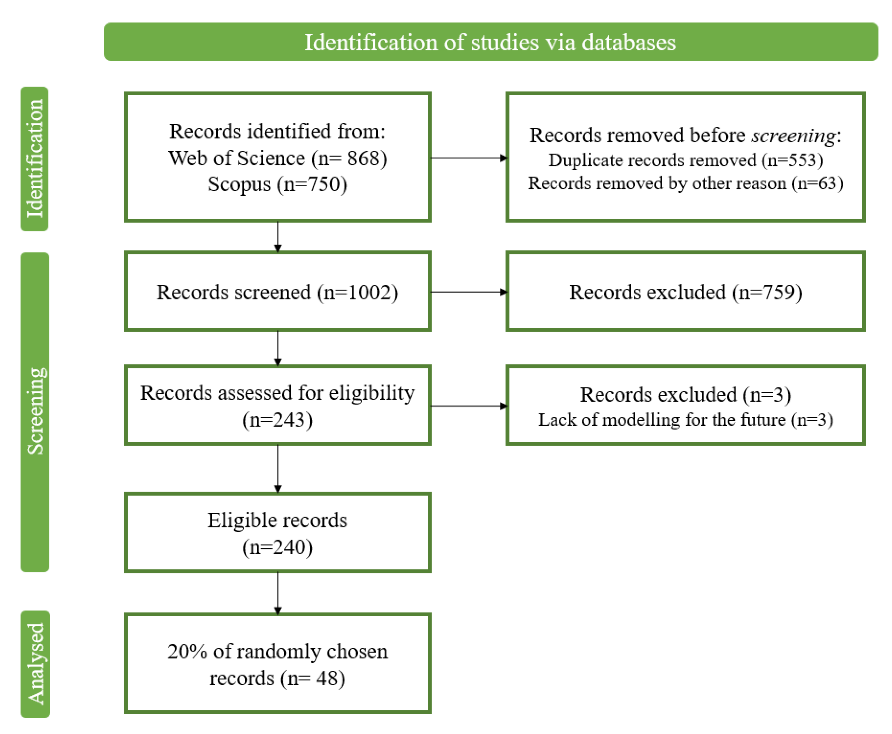
This study aims to identify if best practices are followed when assessing changes in plant species distribution under climate change scenarios based on niche modelling in recent papers. The search was conducted in November 2022 in two databases: Web of Science (WOS) and Scopus. The following search equation was included, using Boolean search strategies: ("climate change" OR "global change") AND ("model*" OR "ecological niche model*" OR "species distribution model*" OR "habitat suitability model*" OR "range shift") AND ("R software" OR "maxent" OR "Biomod*" OR "GLM" OR "average model*" OR "ensemble*") AND ("flora" OR "plant*"). The search was carried out for the item "Topic" in the WOS Core Collection and the "Article title, Abstract, Keywords" topics in Scopus. Since modelling methodologies are constantly changing, a time limit was imposed on the research, considering only scientific papers published from 2018 to 2022. Only original articles were considered and other document types, such as review articles, books or book chapters, were removed. The search was based on PRISMA guidelines [80,81], and the flow chart (Figure 1) resumes the different steps undertaken in the current study.
The duplicate records and articles in other languages besides English were initially removed. Unavailable documents were also excluded. Firstly, the title and abstract of the remaining documents were thoroughly screened and evaluated for inclusion in the study (Figure 1). Secondly, those articles were further assessed according to pre-established exclusion criteria: a) not exclusively focused on terrestrial vascular plant species; b) dedicated to agricultural species and their production, such as vines, rice, and corn; c) on invasive flora; d) on aquatic environments or islands; e) on the evaluation of modelling methods rather than assessing climate change effects on species distributions; and f) lack of modelling for the future.
The screening of the databases found 240 documents complying the selection criteria, and afterwards, a representative sample was randomly selected (20%), a more handable number of articles. Finally, the 48 randomly selected articles were analyzed (Appendix A).
The key aspects of the SDM elements were noted in each selected publication and assembled into a database, i) the source of species occurrence data, ii) the area analyzed, iii) the type of data (presence only, pseudo-absence, absence data), iv) the abiotic variables, v) the variables' selection, vi) the used algorithm (s) for modelling, vii) the model performance metrics, viii) the use of an ensemble model, ix) the climate scenario studied, x) the source of climatic models (databases and GMCs), and, ultimately, xi) the missing description of the used methodology).

3. Results

3.1. Species Occurrence Data

The studies use different data sources for the species occurrence data, and only in one case was this information was missing. The use of one or two combined sources is the most common situation (35.4%), but the combination of three (18.8%) or four (8.3%) data sources was also identified. The most used data source was field survey (62.5%), followed by the use of online databases, such as the Global Biodiversity Information Facility (GBIF) (58.3%) (Figure 2).
For the analyzed studies, 34% considered the total geographic range of the target species, while 66% considered only a fraction, usually delimited by political borders. In almost 44% of the articles, the species' natural geographical range was not presented, and it was unclear if the work considered the species' total range and all the conditions it can endure.
Presence-only data was used in 27% of the papers, while only 4% referred to absence data and 12.5% to pseudo-absence points. In the remaining 56% of the documents, the data type needed to be clarified.

3.2. Abiotic Variables

3.2.1. Climate Variables

Most of the papers (98%) mentioned the source of environmental variables used on models' calibration, and only in one case was the data source not identified. The WorldClim (WorldClim) [82,83] was the most commonly used database for climate data, namely bioclimatic variables, included in 83% of the documents. Usually, the bioclimatic variables were downloaded in two different spatial resolutions: 2.5 minutes (approximately 5 km2) (28%) or 30 seconds (approximately 1 km2) (69.6%). Some studies (15%) used other climatic variables sources, such as Climate Change, Agriculture and Food Security (CCAFS, Data - CCAFS Climate (ccafs-climate.org)) in 8% of the cases, the Africlim [84] (4%), or the ClimateAP (ClimateAP_Map), (2%).

3.2.2. Other Environmental Variables

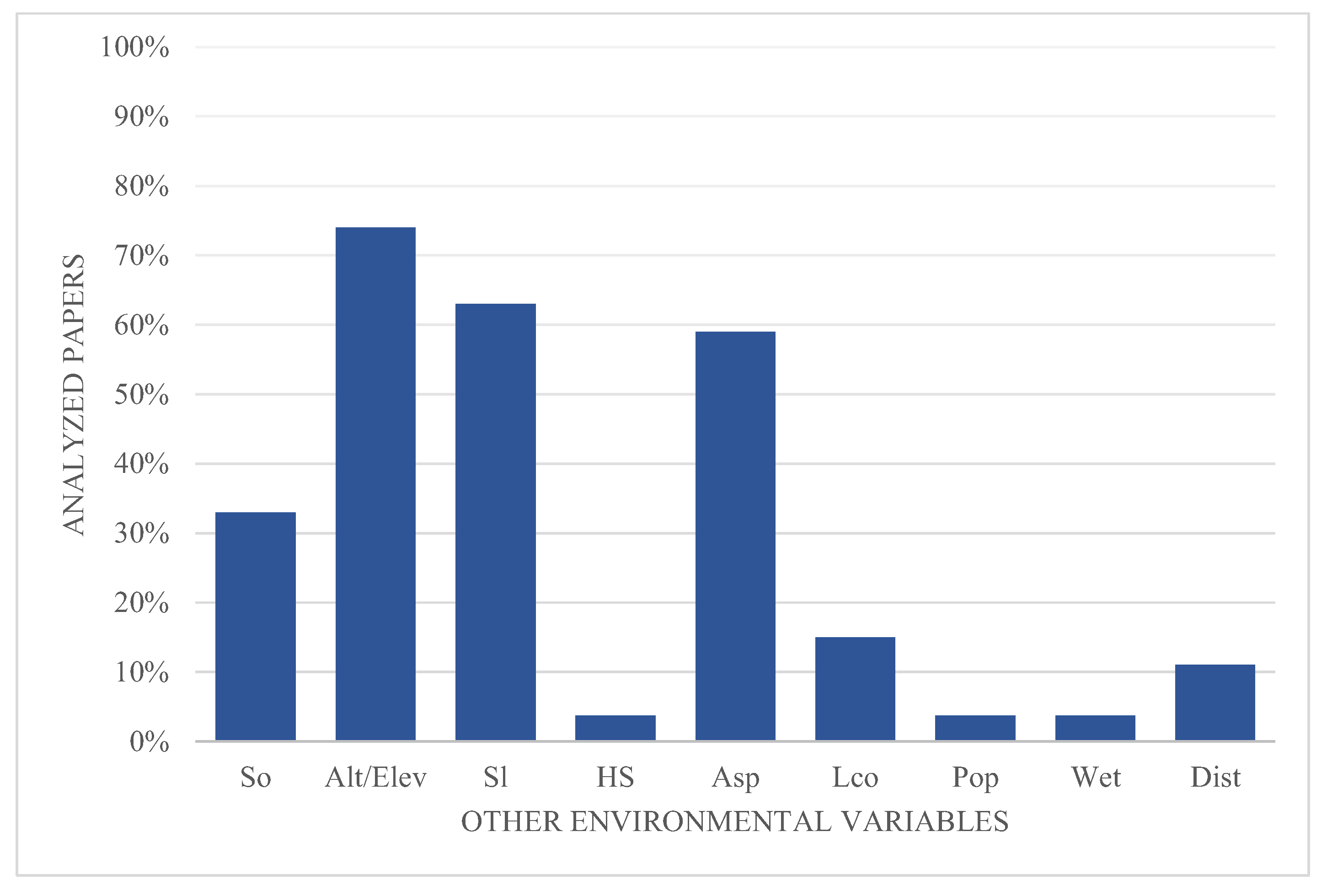
Up to half of the papers (56%) included other variables besides climatic variables. The altitude/elevation was the most common (74%), followed by the slope (63%) and aspect (59%) (Figure 3). In some cases, authors used more specific variables, such as distance to different features, such as rivers and dwellings [85] or fresh and salty water bodies [86].

3.2.3. Variable Selection

The correlation analysis between abiotic variables was performed in 79% of the papers. In comparison, in the remaining papers (21%), no reference was made to the correlation between variables or the methodology used to perform correlation analysis and the variable selection.
In the correlation analysis papers, 54% used Pearson's correlation test. The Variance Inflation Factor (VIF) was also used in 10,5% of the cases. The ArcGIS/ArcMap was used in 8%: in one paper (2%), the band collection statistics analysis was performed in ArcMap, and in two articles the SDMtoolbox was used in different ways - one (2%) used the function 'remove highly correlated variables, and the other the Principal Component Analysis tool. In another case the method used was omitted.

3.3. Modelling Algorithm

In the analyzed papers, eleven different modelling algorithms were used. The MaxEnt was the most popular one, being used in 98% of the cases, and, frequently, was the only one (83% of the cases). Besides MaxEnt, none of the other algorithms was used as the sole algorithm, with 16% of the papers using several different methods. In these cases, the researchers chose to use between four (2%) and ten (4%) algorithms.

3.4. Model Performance

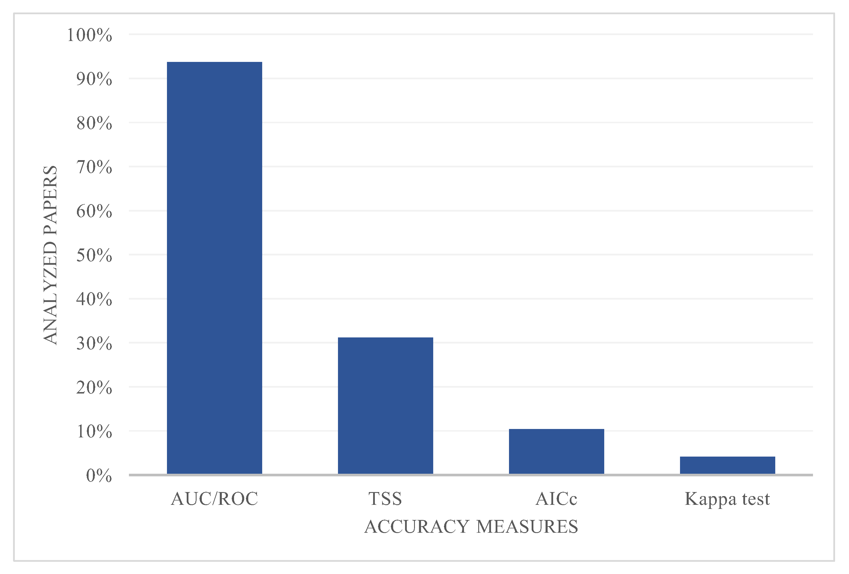
The model's predictive performance was evaluated using four different accuracy measures: the Area Under the Curve of the Receiver Operating Characteristic/ (AUC of ROC), the Akaike's Information Criterion (AICc), the True Skill Statistic (TSS) test and the Cohen's Kappa coefficient. The most used method was the AUC of ROC, mentioned in 93.8% of the articles, the TSS was used in 31.3%, the AICc in 10.4%, and the Cohen's kappa coefficient in 4.2% (Figure 4).
All articles mentioned at least one method to measure model performance. In 62.5% of the cases, only one method was used; in 35.4% the authors opted to use two methods; and in only 2% of the cases, three different methods were used.

3.5. Ensemble Models

In 42% of the papers, only one algorithm and a GCM were used; thus, no ensemble model was produced. In the remaining 58%, where more than one modelling algorithm and/or GCM was used, only 32% created an ensemble model (18.8% of total analyzed papers). The Biomod2 was the package used to perform the ensemble model in 67% of these cases (12.5% of total analyzed papers), with some works using a threshold to choose which models should be considered for the ensemble model.

3.6. Future Climate Projections

3.6.1. Climate Scenarios

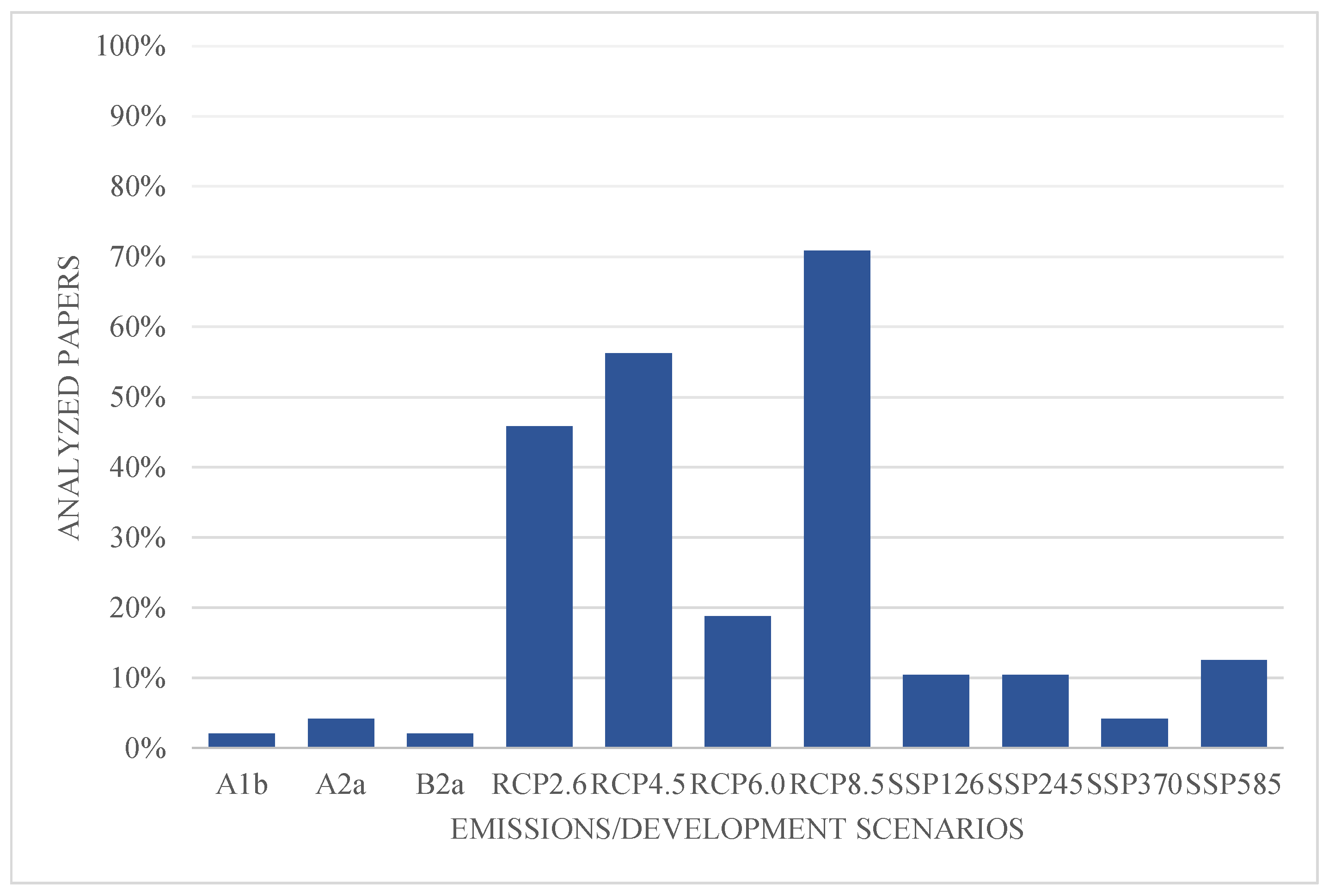
The analyzed papers used mainly two (59.6%) or four different development scenarios (19.1%). The use of one or three different scenarios was less common, and occurred in 8.5% and 12.8% of the cases, respectively. The most popular scenarios were the Representative Concentration Pathways (RCPs): the RCP8.5 (70.8% of the documents), the RCP4.5 (56.3%), and RCP2.6 (45.8%) (Figure 5).
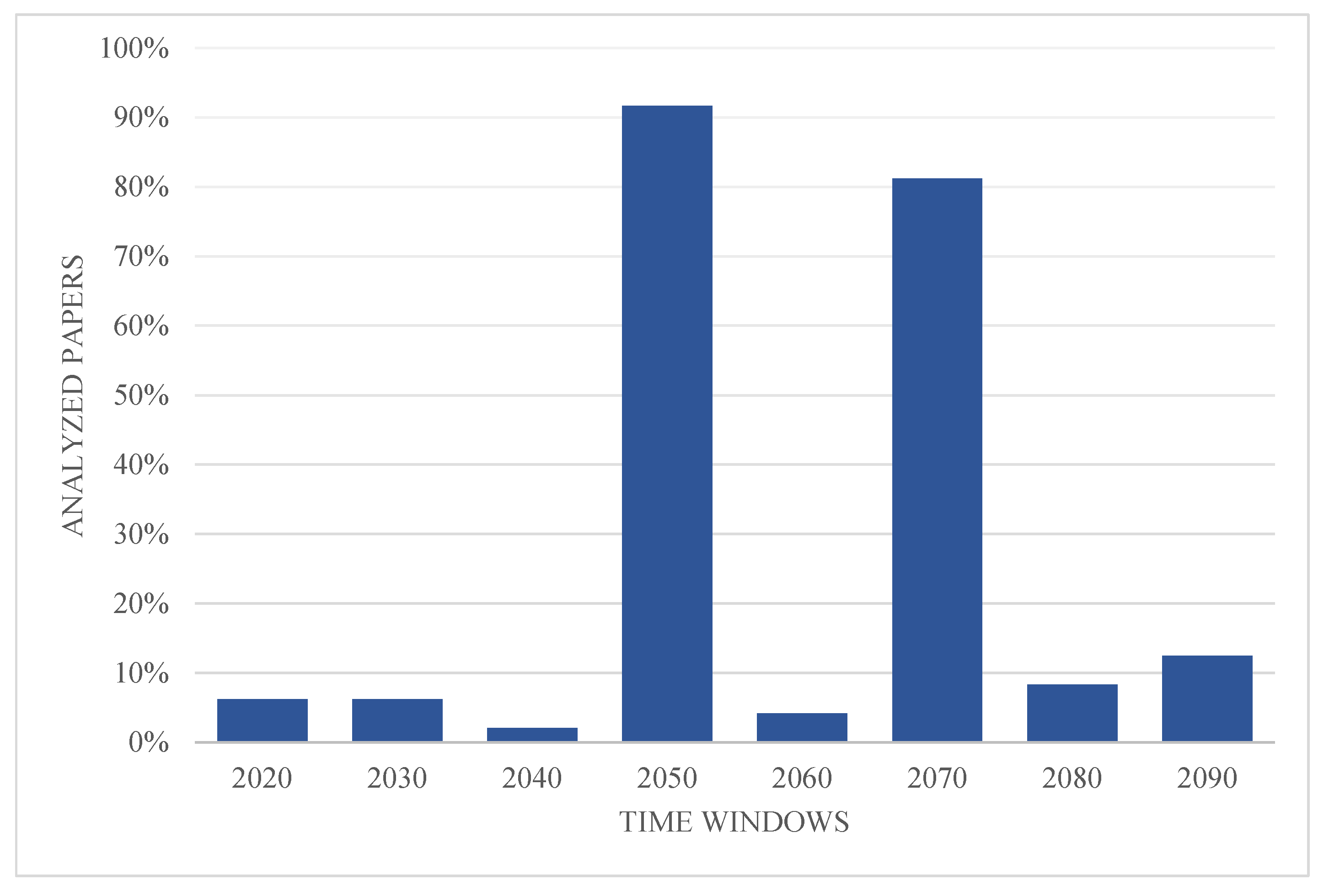
Some future time windows are more popular among flora SDMs papers, namely 2050 (average for 2041–2060) and 2070 (average for 2061–2080), which appear in 91.7% and 81.2% of the documents, respectively (Figure 6). Papers used from one to five different time intervals, with 75% using two different time intervals, and 12.5% using only one.
Summing up, thirty two Global Circulation Models (GCMs) were used in the analyzed documents, considering all versions of several models. In 6% of the cases, the used GCM was not described. In those papers where the used GCM was mentioned, their number ranged from one to eight GCMs, with most papers (64%) using only one GCM to perform the model.
The CCSM4, developed by the National Science Foundation (NSF) and National Centre for Atmospheric Research (NCAR), and the HadGEM2-ES, developed by the UK Meteorological Office, was used in more than 29.8% and 25.5% of the papers, respectively (Table 1). The GCMs developed by the UK Meteorological Office seem to be the most popular (40.4%), followed by the National Science Foundation (NSF), and National Centre for Atmospheric Research (NCAR) (29.8%) and the Beijing Climate Centre Climate System Model (25.5%) (Table 1).

4. Discussion

The information about the methodology used in each work is not always clear and complete. Some parameters are described more consistently, such as the origin of the data. However, many articles fail to specify other parameters, such as the use of absence or pseudo-absence points, ensemble modelling techniques, or even the GCM used. The same tendency, which limits the reproducibility of the studies, was noticed by other authors [1,6,71]. This is a problem that has been addressed in recent literature by several authors, aiming to provide guidelines/checklists for future publications [2,5,6,12]. In addition to the gaps in the description of adopted methodologies, common and recurrent mistakes during SDM application have also been pointed out by recent studies [36,37]. These poor modelling practices can lead to inaccurate conclusions and poor planning of conservation actions [64]. The examined studies had many similarities concerning the different elements analyzed. target species distribution area could have been more clearly stated, either total or partial. Over a third of the papers used the total range of the species, while the rest only considered a fraction. This is an important point, since models that rely on partial distributions may not be able to capture the full range of abiotic conditions in which a species can survive [2], and marginal populations can have adaptations to more extreme situations [51]. It is also essential to include location conditions that do not yet exist, in the study area (e.g. using buffer zones), but will probably exist, so that the model can assess the suitability of these conditions in the future. Ignoring this can lead to errors since the model cannot make accurate projections for unknown climatic conditions [32,33]. However, this seems common in ecological modelling exercises [53,54,55]. For this reason, niche truncation and clamping can lead to incorrect predictions when projecting to future climatic conditions, since future conditions may be unavailable in the calibration area, but may be suitable for the species [39,53,55]. This can result in predicting false local extinctions or extirpations and, hence, inaccurate predictions of future species suitability, especially at range margins [50]. However, excluding areas under a climate that will no longer exist in the future, e.g. the northern range limit of a European species, may not be problematic, since those conditions will no longer be present [50]. The explanation of the species' range and the study area should be well specified, together with the reasons for those choices [25], which was not always the case. Nevertheless, only one work addressed superficially niche truncation.
Field surveys were the most popular data source, but performing models only with field data can lead to problems related to some areas being over-sampled, especially when species have a broad range area [31]. Although systematically designed surveys covering major species ranges are recommended [5], systematic surveys along all species range areas in major environmental gradients occupied can be source-demanding, expensive and time-consuming [36,40]. On the other hand, opportunistic sampling (e.g. GBIF) can have other problems, such as the misidentification of species, and spatial bias records due to uneven effort of sampling [28,34], but larger sample size of these type of data seems to compensate and outperforms systematic sampling [89,90,91]. These biases and inaccuracies in distributional data can place heavy limitations on SDM studies and affect the quality of final results [5]. About two-thirds of the studies used more than one source for occurrence data gathering, from fieldwork and large databases to locations mentioned in specific studies or herbaria. This can be a good strategy since the more information is given to the model, the better it will perform [92] and data from different sources might complement each other [89]. Also, when sample data are collected from broad geographical areas, including different environmental gradients, a higher possibility exists that environmental conditions limiting species distribution will be well sampled [24].
The climate variables were used in all studies and the most common source was WorldClim, which was included in a large majority of the papers. The models were performed mainly at a 30 seconds spatial resolution (approximately ~1 km2), the highest resolution used. Although, depending on the study goal or for small-range species, a finer special scale should be used [58]. The 30 seconds scale is often the finer available scale, which limits the possibility of performing finer scale models. Larger scale models may detect less variation in topography or soil conditions compared with finer-scale data, resulting in a lower ability for the models to discern topographic and soil variation within the landscape [58].
However, non-climactic factors might also influence plant species distribution [35,56,57]. Circa half of the analyzed studies used climatic variables only. Other environmental variables were not included in the model, which can overestimate habitat suitability for many plant species, both in the present and under future scenarios, since climate-based projections might integrate areas with unsuitable soil conditions [57]. Some of these studies highlight this fact, pointing to this issue as a limitation [93,94], and others argue a lack of reliable data on a scale that would allow their inclusion in the model. Yet, including all climate and non-climate variables in the same models may not always be suitable [6], since these variables may be highly correlated [61], and their correlation can change through time [37] making future projections less reliable.
Indeed, variable selection is a crucial step in SDM, but one-fifth of the analyzed articles lack to mention variable selection or do not describe the method used. Some simply use all the variables to perform models, without considering possible present and future correlations between them. Even though, most modelling algorithms are sensitive to high levels of correlation between variables. MaxEnt, the most used algorithm in the analyzed papers, seems to be capable of dealing with redundant variables and the independence between the degree of predictor collinearity and collinearity shift [60]. So, the strategy of removing highly correlated variables seems to have a small impact on MaxEnt model performance [60]. The articles that do not refer to variable selection used mainly MaxEnt. However, in those using other algorithms (BRT, RF, GLM, GAM, MARS and CTA) no justification is given for the absence of correlation analysis and variable selection. The variable selection based on correlation should be performed to simplify the interpretation of the model [64]. Additionally, the species' ecological preferences should be considered, to select the most meaningful variables to be included in the model [24,30,66,67,95].
Several methods are available to perform SDMs, no single one is superior in all situations [70,71] and they seem to have similar performances [92]. Even though, BRT, MaxEnt, and RF were reported to be the best-performing modelling algorithms, while parametric and semi-parametric regression models (like GLM and GAM) can be good choices when the number of occurrences is very low [70]. In accordance with other similar ones [71,96], MaxEnt was by far the most used algorithm in the screened studies, as previously said. Though, the percentage of papers using this algorithm was larger in our review than in others [71,96], and the only used algorithm in most papers. The MaxEnt is a machine-learning method [97,98], and some of its features can contribute to its popularity compared to other algorithms: is user-friendly, even for a beginner user; outputs are easy to access and read; it is very accessible, it can be used in open-source software or on free software R programming packages; there is no need to provide absence points and it generates significant results with a small number and spatially biased presence points, it is shown to deliver good results [2,58,70,97,98,99,100]. Despite that, in climate change assessments and future projections, it seems advisable to use more than one algorithm to produce a final model, according to consensual best practices [5].
Most papers used more than one climate scenario and more than one time interval. The Shared Socioeconomic Pathways (SSPs) [42] are notably less used than RCPs [88], probably because they are more recent and unavailable when some of these works were developed. On the other hand, the scenarios provided by [87] had shallow usage, which makes sense, as more robust scenarios were available when these papers were published. The RCP8.5 was the most used scenario, although it describes a situation with very high anthropogenic greenhouse gas emissions without additional efforts to constrain them [88]. Papers using this scenario also used at least other intermediate scenarios. Most screened papers displayed two different future time intervals, and a preference exists for more distant temporal periods. This makes sense and might be helpful when the goal is to plan management actions, especially for long-living species. Adaptive and management strategies require a longer-term perspective since areas managed nowadays must cope with the future climate conditions of at least several decades [101,102]. However, many species may not yet be able to be established in places that will only be suitable in a few decades. Therefore, not-so-distant periods might also provide meaningful information about transition areas.
The verified studies used a wide range of GCMs, a total of 32 considering all versions of the models, with most articles using only one GCM to perform the analysis. Since GCMs are projections and prone to errors, using more than one GCM has been emphasized to reduce uncertainty when projecting species distribution in time [29,49]. Still, more than one-third of the papers used more than one GCM: from 2 to 8. Some GCMs are more used than others. Those developed by the UK Meteorological Office are the most popular, followed by the National Science Foundation (NSF) and National Centre for Atmospheric Research (NCAR) from the United States and the Beijing Climate Centre Climate System Model, from the People's Republic of China.
When several algorithms or GCMs were used, ensemble models were often performed, in less than a fifth of the articles. Ensemble modelling is often considered to have better predictive results and to be more reliable than single models and is often used to reduce the degree of uncertainty in the model selection [1,70,71]. Still, performing an ensemble using models with good and bad predictive capacity may not result in a good final model [2]. Similarly, to other works [1] and likewise in other analyzed parameters, the methodology for performing the ensemble is sparsely described in the analyzed works. Only two-thirds of the articles performing ensembles clearly stated the use of Biomod2, and only one-third described the choice of the best models to include in the ensemble, using a threshold, based on AUC or TSS.
A large majority of the papers used ROC/AUC to measure model performance. Although over a third of the studies used more than one method, often in a complementary way, the use of the AUC stands out. This holds true in another study [74] and is possibly related to non-threshold dependency of the ROC/AUC, which is a metric provided by MaxEnt and is used in a wide range of applications related to producing predictions. Despite its wider use, the single use of AUC, or another single metric, can misidentify over-fitted models as well-fitting and strongly predictive [48], therefore models should be carefully evaluated by specialists, to check whether they make sense ecologically for the target species [103].

5. Conclusions

The current review identified 240 papers modelling plant species niches and possible future range shifts due to climate change, 48 of which were randomly selected and analyzed. Despite published standards for the use of niche models, recent studies focused on climate change still exhibit uncertainty related to inconsistent methodological decisions. Although modelling strategies and data sources are pretty consistent, the methodology is sometimes missing, which hinders the reproducibility of SDM studies and increases uncertainty considering the discussion of results.
Species occurrence data comprise mainly part of the species range and use more than just one source, with field surveys being the most popular choice. All papers used climate data, but other environmental variables were used in over half of the documents.
The choice of modelling algorithm was quite homogeneous, almost all documents using MaxEnt, often the only used algorithm. Using only one GCM was a popular choice although a best practice to use more than one, but no clear preference was found for a particular GCM.
The parameters analysis indicates that several articles base their models on several choices that may lead to inaccurate and possibly unreliable results. The definition of a study area not including the whole species' natural range, leaving out areas and environments in which the species can live and that have climatic conditions that might be more usual in the future, was common since over half of the studies only considered a part of the species range. Also, ignoring species' ecological preferences when choosing the variables to use in the model, both at the outset and after variables' selection, is another error that appears to be common, and which can lead to putative inaccuracies in the results.
Overall, there is a need to make the information clearer and more comprehensive in the SDM studies. In this paper, we emphasize that the information regarding the species being studied and the modelling process is often missing. Therefore, besides best practices referred to in guidelines papers previously cited, it is considered pertinent in future modelling studies to include and state the following information:
  • Target species natural range;
  • Considering the total species range in the study area, including a buffer to ensure the inclusion of different environmental conditions;
  • Compare the study area and the natural range of the species, and justify the exclusion of certain areas from the model, if this is the case;
  • Species' ecological preferences according to the bibliography, to support the selection variables selection;
Whatever the author's options, in the papers there should be a greater criticism of the obtained results, identifying putative constraints that may influence final results and which points can be improved in future studies.

Supplementary Materials

The following supporting information can be downloaded at the website of this paper posted on Preprints.org, Appendix A.

Author Contributions

Isabel Passos: Conceptualization, Methodology, Writing – original draft. Albano Figueiredo: Conceptualization, Writing – review & editing, Supervision. Alice Almeida: Writing – review & editing; Maria Margarida Ribeiro; Writing – review & editing.

Funding

This work was supported by national funds through the Portuguese Foundation for Science and Technology (FCT) under the grant UI/BD/152853/2022, projects CERNAS-IPCB (UIDB/00681/2020), CEF (UIDB/00239/2020), and the Centre of Studies in Geography and Spatial Planning (CEGOT) (UIDP/GEO/04084/2020_UC).

Data Availability Statement

Data are not yet provided, due to the impossibility of having restricted access in our repository, but will be archived upon acceptance.

Conflicts of Interest

The authors declare that they have no known competing financial interests or personal relationships that could have appeared to influence the work reported in this paper.

Appendix A

The appendix contains the articles analyzed within this review.

References

  1. T. Hao, J. Elith, G. Guillera-Arroita, and J. J. Lahoz-Monfort, “A review of evidence about use and performance of species distribution modelling ensembles like BIOMOD,” Diversity and Distributions, vol. 25, no. 5. Blackwell Publishing Ltd, pp. 839–852, May 01, 2019. [CrossRef]
  2. N. Sillero et al., “Want to model aspecies niche? A step-by-step guideline on correlative ecological niche modelling,” Ecol Modell, vol. 456, Sep. 2021. [CrossRef]
  3. J. Elith and J. R. Leathwick, “Species distribution models: Ecological explanation and prediction across space and time,” Annu Rev Ecol Evol Syst, vol. 40, pp. 677–697, Dec. 2009. [CrossRef]
  4. G. Guillera-Arroita, “Modelling of species distributions, range dynamics and communities under imperfect detection: advances, challenges and opportunities,” Ecography, vol. 40, no. 2, pp. 281–295, Feb. 2017. [CrossRef]
  5. M. B. Araújo et al., “Standards for distribution models in biodiversity assessments,” Sci Adv, vol. 5, no. 1, Jan. 2019. [CrossRef]
  6. X. Feng, D. S. Park, C. Walker, A. T. Peterson, C. Merow, and M. Papeş, “A checklist for maximizing reproducibility of ecological niche models,” Nat Ecol Evol, vol. 3, no. 10, pp. 1382–1395, Oct. 2019. [CrossRef]
  7. E. Gómez-Pineda, A. Blanco-García, R. Lindig-Cisneros, G. A. O’Neill, L. Lopez-Toledo, and C. Sáenz-Romero, “Pinus pseudostrobus assisted migration trial with rain exclusion: maintaining Monarch Butterfly Biosphere Reserve forest cover in an environment affected by climate change,” New For (Dordr), vol. 52, no. 6, pp. 995–1010, Nov. 2021. [CrossRef]
  8. C. Guo, S. Lek, S. Ye, W. Li, J. Liu, and Z. Li, “Uncertainty in ensemble modelling of large-scale species distribution: Effects from species characteristics and model techniques,” Ecol Modell, vol. 306, pp. 67–75, Jun. 2015. [CrossRef]
  9. C. Merow et al., “What do we gain from simplicity versus complexity in species distribution models?,” Ecography, vol. 37, no. 12, pp. 1267–1281, Dec. 2014. [CrossRef]
  10. Y. Shen et al., “Predicting the impact of climate change on the distribution of two relict Liriodendron species by coupling the MaxEnt model and actual physiological indicators in relation to stress tolerance,” J Environ Manage, vol. 322, Nov. 2022. [CrossRef]
  11. F. Xiao, Y. She, J. She, J. Zhang, X. Zhang, and C. Luo, “Assessing habitat suitability and selecting optimal habitats for relict tree Cathaya argyrophylla in Hunan, China: Integrating pollen size, environmental factors, and niche modeling for conservation,” Ecol Indic, vol. 145, Dec. 2022. [CrossRef]
  12. D. Zurell et al., “A standard protocol for reporting species distribution models,” Ecography, vol. 43, no. 9, pp. 1261–1277, Sep. 2020. [CrossRef]
  13. M. Pecchi et al., “Species distribution modelling to support forest management. A literature review,” Ecological Modelling, vol. 411. Elsevier B.V., Nov. 01, 2019. [CrossRef]
  14. P. Bogawski et al., “Current and future potential distributions of three Dracaena Vand. ex L. species under two contrasting climate change scenarios in Africa,” Ecol Evol, vol. 9, no. 12, pp. 6833–6848, Jun. 2019. [CrossRef]
  15. S. Jian, T. Zhu, J. Wang, and D. Yan, “The Current and Future Potential Geographical Distribution and Evolution Process of Catalpa bungei in China,” Forests, vol. 13, no. 1, Jan. 2022. [CrossRef]
  16. A. M. Almeida et al., “Prediction scenarios of past, present, and future environmental suitability for the Mediterranean species Arbutus unedo L.,” Sci Rep, vol. 12, no. 1, Dec. 2022. [CrossRef]
  17. K. Dimobe et al., “Climate change reduces the distribution area of the shea tree (Vitellaria paradoxa C.F. Gaertn.) in Burkina Faso,” J Arid Environ, vol. 181, Oct. 2020. [CrossRef]
  18. E. A. Farahat and A. M. Refaat, “Predicting the impacts of climate change on the distribution of Moringa peregrina (Forssk.) Fiori — A conservation approach,” J Mt Sci, vol. 18, no. 5, pp. 1235–1245, May 2021. [CrossRef]
  19. D. Kumar, S. Rawat, and R. Joshi, “Predicting the current and future suitable habitat distribution of the medicinal tree Oroxylum indicum (L.) Kurz in India,” J Appl Res Med Aromat Plants, vol. 23, May 2021. [CrossRef]
  20. A. J. Mendoza-Fernández et al., “The relict ecosystem of maytenus senegalensis subsp. europaea in an agricultural landscape: Past, present and future scenarios,” Land (Basel), vol. 10, no. 1, pp. 1–15, Jan. 2021. [CrossRef]
  21. S. K. Rana, H. K. Rana, J. Stöcklin, S. Ranjitkar, H. Sun, and B. Song, “Global warming pushes the distribution range of the two alpine ‘glasshouse’ Rheum species north- and upwards in the Eastern Himalayas and the Hengduan Mountains,” Front Plant Sci, vol. 13, Oct. 2022. [CrossRef]
  22. G. Tessarolo, J. M. Lobo, T. F. Rangel, and J. Hortal, “High uncertainty in the effects of data characteristics on the performance of species distribution models,” Ecol Indic, vol. 121, Feb. 2021. [CrossRef]
  23. D. L. Warren, A. Dornburg, K. Zapfe, and T. L. Iglesias, “The effects of climate change on Australia’s only endemic Pokémon: Measuring bias in species distribution models,” Methods Ecol Evol, vol. 12, no. 6, pp. 985–995, Jun. 2021. [CrossRef]
  24. M. B. Araújo and A. Guisan, “Five (or so) challenges for species distribution modelling,” J Biogeogr, vol. 33, no. 10, pp. 1677–1688, Oct. 2006. [CrossRef]
  25. M. B. Araújo and A. T. Peterson, “Uses and misuses of bioclimatic envelope models,” 2012.
  26. M. Fernandez, H. Hamilton, and L. M. Kueppers, “Characterizing uncertainty in species distribution models derived from interpolated weather station data,” Ecosphere, vol. 4, no. 5, May 2013. [CrossRef]
  27. R. K. Heikkinen, M. Luoto, M. B. Araújo, R. Virkkala, W. Thuiller, and M. T. Sykes, “Methods and uncertainties in bioclimatic envelope modelling under climate change,” Progress in Physical Geography, vol. 30, no. 6. Arnold, pp. 751–777, 2006. [CrossRef]
  28. J. Beck, M. Böller, A. Erhardt, and W. Schwanghart, “Spatial bias in the GBIF database and its effect on modeling species’ geographic distributions,” Ecol Inform, vol. 19, pp. 10–15, 2014. [CrossRef]
  29. N. Casajus, C. Périé, T. Logan, M. C. Lambert, S. de Blois, and D. Berteaux, “An objective approach to select climate scenarios when projecting species distribution under climate change,” PLoS One, vol. 11, no. 3, Mar. 2016. [CrossRef]
  30. C. F. Dormann et al., “Correlation and process in species distribution models: bridging a dichotomy.,” J Biogeogr, vol. 39, no. 12, pp. 2119–2131, 2013. [CrossRef]
  31. Y. Fourcade, J. O. Engler, D. Rödder, and J. Secondi, “Mapping species distributions with MAXENT using a geographically biased sample of presence data: A performance assessment of methods for correcting sampling bias,” PLoS One, vol. 9, no. 5, May 2014. [CrossRef]
  32. L. Guevara, B. E. Gerstner, J. M. Kass, and R. P. Anderson, “Toward ecologically realistic predictions of species distributions: A cross-time example from tropical montane cloud forests,” Glob Chang Biol, vol. 24, no. 4, pp. 1511–1522, Apr. 2018. [CrossRef]
  33. L. Guevara and L. León-Paniagua, “How to survive a glaciation: the challenge of estimating biologically realistic potential distributions under freezing conditions,” Ecography, vol. 42, no. 6, pp. 1237–1245, Jun. 2019. [CrossRef]
  34. B. M. Marshall and C. T. Strine, “Exploring snake occurrence records: Spatial biases and marginal gains from accessible social media,” PeerJ, vol. 2019, no. 12, 2019. [CrossRef]
  35. P. W. Moonlight et al., “The strengths and weaknesses of species distribution models in biome delimitation,” Global Ecology and Biogeography, vol. 29, no. 10, pp. 1770–1784, Oct. 2020. [CrossRef]
  36. D. Rocchini et al., “Anticipating species distributions: Handling sampling effort bias under a Bayesian framework,” Science of the Total Environment, vol. 584–585, pp. 282–290, Apr. 2017. [CrossRef]
  37. N. Sillero and A. M. Barbosa, “Common mistakes in ecological niche models,” International Journal of Geographical Information Science, vol. 35, no. 2. Taylor and Francis Ltd., pp. 213–226, 2020. [CrossRef]
  38. L. D. Silva, E. B. de Azevedo, F. V. Reis, R. B. Elias, and L. Silva, “Limitations of species distribution models based on available climate change data: A case study in the azorean forest,” Forests, vol. 10, no. 7, Jul. 2019. [CrossRef]
  39. T. J. Stohlgren, C. S. Jarnevich, W. E. Esaias, and J. T. Morisette, “Bounding species distribution models,” 2011. [Online]. Available: http://groups.google.com/group/maxent/.
  40. M. M. ElQadi, A. Dorin, A. Dyer, M. Burd, Z. Bukovac, and M. Shrestha, “Mapping species distributions with social media geo-tagged images: Case studies of bees and flowering plants in Australia,” Ecol Inform, vol. 39, pp. 23–31, May 2017. [CrossRef]
  41. R. P. Anderson et al., “Report of the task group on GBIF data fitness for use in distribution modelling,” 2016. [Online]. Available: http://www.gbif.org.
  42. IPCC, Climate Change 2022 – Impacts, Adaptation and Vulnerability. Contribution of Working Group II to the Sixth Assessment Report of the Intergovernmental Panel on Climate Change. Cambridge, UK and New York, NY, USA: Cambridge University Press, 2022. [CrossRef]
  43. B. C. O’Neill et al., “The Scenario Model Intercomparison Project (ScenarioMIP) for CMIP6,” Geosci Model Dev, vol. 9, no. 9, pp. 3461–3482, Sep. 2016. [CrossRef]
  44. R. H. Moss et al., “The next generation of scenarios for climate change research and assessment,” Nature, vol. 463, no. 7282. pp. 747–756, Feb. 11, 2010. [CrossRef]
  45. K. Riahi et al., “The Shared Socioeconomic Pathways and their energy, land use, and greenhouse gas emissions implications: An overview,” Global Environmental Change, vol. 42, pp. 153–168, Jan. 2017. [CrossRef]
  46. D. P. van Vuuren et al., “The representative concentration pathways: An overview,” Clim Change, vol. 109, no. 1, pp. 5–31, Nov. 2011. [CrossRef]
  47. B. C. O’Neill et al., “Achievements and needs for the climate change scenario framework,” Nat Clim Chang, vol. 10, no. 12, pp. 1074–1084, Dec. 2020. [CrossRef]
  48. C. M. Beale and J. J. Lennon, “Incorporating uncertainty in predictive species distribution modelling,” Philosophical Transactions of the Royal Society B: Biological Sciences, vol. 367, no. 1586. Royal Society, pp. 247–258, Jan. 19, 2012. [CrossRef]
  49. C. F. McSweeney, R. G. Jones, R. W. Lee, and D. P. Rowell, “Selecting CMIP5 GCMs for downscaling over multiple regions,” Clim Dyn, vol. 44, no. 11–12, pp. 3237–3260, Jun. 2015. [CrossRef]
  50. M. Barbet-Massin, W. Thuiller, and F. Jiguet, “How much do we overestimate future local extinction rates when restricting the range of occurrence data in climate suitability models?,” Ecography, vol. 33, no. 5, pp. 878–886, Oct. 2010. [CrossRef]
  51. A. Lázaro-Nogal, S. Matesanz, L. Hallik, A. Krasnova, A. Traveset, and F. Valladares, “Population differentiation in a Mediterranean relict shrub: the potential role of local adaptation for coping with climate change,” Oecologia, vol. 180, no. 4, pp. 1075–1090, Apr. 2016. [CrossRef]
  52. N. Titeux et al., “The need for large-scale distribution data to estimate regional changes in species richness under future climate change,” Divers Distrib, vol. 23, no. 12, pp. 1393–1407, Dec. 2017. [CrossRef]
  53. M. Chevalier, O. Broennimann, J. Cornuault, and A. Guisan, “Data integration methods to account for spatial niche truncation effects in regional projections of species distribution,” Ecological Applications, vol. 31, no. 7, Oct. 2021. [CrossRef]
  54. M. Chevalier, A. Zarzo-Arias, J. Guélat, R. G. Mateo, and A. Guisan, “Accounting for niche truncation to improve spatial and temporal predictions of species distributions,” Front Ecol Evol, vol. 10, Aug. 2022. [CrossRef]
  55. D. Scherrer, M. Esperon-Rodriguez, L. J. Beaumont, V. L. Barradas, and A. Guisan, “National assessments of species vulnerability to climate change strongly depend on selected data sources,” Divers Distrib, vol. 27, no. 8, pp. 1367–1382, Aug. 2021. [CrossRef]
  56. F. O. G. Figueiredo, G. Zuquim, H. Tuomisto, G. M. Moulatlet, H. Balslev, and F. R. C. Costa, “Beyond climate control on species range: The importance of soil data to predict distribution of Amazonian plant species,” J Biogeogr, vol. 45, no. 1, pp. 190–200, Jan. 2018. [CrossRef]
  57. G. Zuquim, F. R. C. Costa, H. Tuomisto, G. M. Moulatlet, and F. O. G. Figueiredo, “The importance of soils in predicting the future of plant habitat suitability in a tropical forest,” Plant Soil, vol. 450, no. 1–2, pp. 151–170, May 2020. [CrossRef]
  58. C. Rovzar, T. W. Gillespie, and K. Kawelo, “Landscape to site variations in species distribution models for endangered plants,” For Ecol Manage, vol. 369, pp. 20–28, Jun. 2016. [CrossRef]
  59. S. J. E. Velazco, F. Galvão, F. Villalobos, and P. De Marco, “Using worldwide edaphic data to model plant species niches: An assessment at a continental extent,” PLoS One, vol. 12, no. 10, Oct. 2017. [CrossRef]
  60. X. Feng, D. S. Park, Y. Liang, R. Pandey, and M. Papeş, “Collinearity in ecological niche modeling: Confusions and challenges,” Ecol Evol, vol. 9, no. 18, pp. 10365–10376, Sep. 2019. [CrossRef]
  61. R. Sehler, J. Li, J. Reager, and H. Ye, “Investigating Relationship Between Soil Moisture and Precipitation Globally Using Remote Sensing Observations,” J Contemp Water Res Educ, vol. 168, no. 1, pp. 106–118, Dec. 2019. [CrossRef]
  62. S. de Tomás Marín et al., “Fagus sylvatica and Quercus pyrenaica: Two neighbors with few things in common,” For Ecosyst, vol. 10, Jan. 2023. [CrossRef]
  63. Y. Vitasse, C. C. Bresson, A. Kremer, R. Michalet, and S. Delzon, “Quantifying phenological plasticity to temperature in two temperate tree species,” Funct Ecol, vol. 24, no. 6, pp. 1211–1218, Dec. 2010. [CrossRef]
  64. P. García-Díaz, T. A. A. Prowse, D. P. Anderson, M. Lurgi, R. N. Binny, and P. Cassey, “A concise guide to developing and using quantitative models in conservation management,” Conserv Sci Pract, vol. 1, no. 2, p. e11, Feb. 2019. [CrossRef]
  65. C. F. Dormann et al., “Collinearity: A review of methods to deal with it and a simulation study evaluating their performance,” Ecography, vol. 36, no. 1, pp. 27–46, 2013. [CrossRef]
  66. B. Petitpierre, O. Broennimann, C. Kueffer, C. Daehler, and A. Guisan, “Selecting predictors to maximize the transferability of species distribution models: lessons from cross-continental plant invasions.,” Global Ecology and Biogeography, vol. 26, no. 3, pp. 275–287, 2017. [CrossRef]
  67. E. P. Tanner, M. Papeş, R. D. Elmore, S. D. Fuhlendorf, and C. A. Davis, “Incorporating abundance information and guiding variable selection for climate-based ensemble forecasting of species’ distributional shifts,” PLoS One, vol. 12, no. 9, Sep. 2017. [CrossRef]
  68. M. Barbet-Massin, F. Jiguet, C. H. Albert, and W. Thuiller, “Selecting pseudo-absences for species distribution models: How, where and how many?,” Methods Ecol Evol, vol. 3, no. 2, pp. 327–338, Apr. 2012. [CrossRef]
  69. M. Guerrina, E. Conti, L. Minuto, and G. Casazza, “Knowing the past to forecast the future: a case study on a relictual, endemic species of the SW Alps, Berardia subacaulis,” Reg Environ Change, vol. 16, no. 4, pp. 1035–1045, Apr. 2015. [CrossRef]
  70. R. Valavi, G. Guillera-Arroita, J. J. Lahoz-Monfort, and J. Elith, “Predictive performance of presence-only species distribution models: a benchmark study with reproducible code,” Ecol Monogr, vol. 92, no. 1, Feb. 2022. [CrossRef]
  71. A. W. Qazi, Z. Saqib, and M. Zaman-ul-Haq, “Trends in species distribution modelling in context of rare and endemic plants: a systematic review,” Ecological Processes, vol. 11, no. 1. Springer Science and Business Media Deutschland GmbH, Dec. 01, 2022. [CrossRef]
  72. D. F. Alvarado-Serrano and L. L. Knowles, “Ecological niche models in phylogeographic studies: Applications, advances and precautions,” Mol Ecol Resour, vol. 14, no. 2, pp. 233–248, Mar. 2014. [CrossRef]
  73. R. Sor, Y. S. Park, P. Boets, P. L. M. Goethals, and S. Lek, “Effects of species prevalence on the performance of predictive models,” Ecol Modell, vol. 354, pp. 11–19, Jun. 2017. [CrossRef]
  74. C. R. Lawson, J. A. Hodgson, R. J. Wilson, and S. A. Richards, “Prevalence, thresholds and the performance of presence-absence models,” Methods Ecol Evol, vol. 5, no. 1, pp. 54–64, Jan. 2014. [CrossRef]
  75. J. M. Lobo, A. Jiménez-valverde, and R. Real, “AUC: A misleading measure of the performance of predictive distribution models,” Global Ecology and Biogeography, vol. 17, no. 2. pp. 145–151, Mar. 2008. [CrossRef]
  76. H. R. Sofaer, J. A. Hoeting, and C. S. Jarnevich, “The area under the precision-recall curve as a performance metric for rare binary events,” Methods Ecol Evol, vol. 10, no. 4, pp. 565–577, Apr. 2019. [CrossRef]
  77. A. Jiménez-Valverde, “Insights into the area under the receiver operating characteristic curve (AUC) as a discrimination measure in species distribution modelling,” Global Ecology and Biogeography, vol. 21, no. 4, pp. 498–507, Apr. 2012. [CrossRef]
  78. B. Leroy, R. Delsol, B. Hugueny, C. N. Meynard, M. Barbet-Massin, and C. Bellard, “Title: Without quality presence-absence data, discrimination metrics such as TSS can be misleading measures of model performance 4 5 Word count: 3719 (without references) ; 5123 (with references)”. [CrossRef]
  79. G. Rapacciuolo, “Strengthening the contribution of macroecological models to conservation practice,” Global Ecology and Biogeography, vol. 28, no. 1, pp. 54–60, Jan. 2019. [CrossRef]
  80. M. J. Page et al., “The PRISMA 2020 statement: An updated guideline for reporting systematic reviews,” PLoS Medicine, vol. 18, no. 3. Public Library of Science, Mar. 29, 2021. [CrossRef]
  81. M. J. Page et al., “PRISMA 2020 explanation and elaboration: Updated guidance and exemplars for reporting systematic reviews,” The BMJ, vol. 372. BMJ Publishing Group, Mar. 29, 2021. [CrossRef]
  82. S. E. Fick and R. J. Hijmans, “WorldClim 2: new 1-km spatial resolution climate surfaces for global land areas,” International Journal of Climatology, vol. 37, no. 12, pp. 4302–4315, Oct. 2017. [CrossRef]
  83. R. J. Hijmans, S. E. Cameron, J. L. Parra, P. G. Jones, and A. Jarvis, “Very high resolution interpolated climate surfaces for global land areas,” International Journal of Climatology, vol. 25, no. 15, pp. 1965–1978, Dec. 2005. [CrossRef]
  84. P. J. Platts, P. A. Omeny, and R. Marchant, “AFRICLIM: high-resolution climate projections for ecological applications in Africa,” Afr J Ecol, vol. 53, no. 1, pp. 103–108, 2015. [CrossRef]
  85. H. G. Wouyou, B. E. Lokonon, R. Idohou, A. G. Zossou-Akete, A. E. Assogbadjo, and R. Glèlè Kakaï, “Predicting the potential impacts of climate change on the endangered Caesalpinia bonduc (L.) Roxb in Benin (West Africa),” Heliyon, vol. 8, no. 3, Mar. 2022. [CrossRef]
  86. J. Xiao, A. Eziz, H. Zhang, Z. Wang, Z. Tang, and J. Fang, “Responses of four dominant dryland plant species to climate change in the Junggar Basin, northwest China,” Ecol Evol, vol. 9, no. 23, pp. 13596–13607, Dec. 2019. [CrossRef]
  87. IPCC, Climate Change 2007: Synthesis Report. Contribution of Working Groups I, II and III to the Fourth Assessment Report of the Intergovernmental Panel on Climate Change. Geneva: Intergovernmental Panel on Climate Change, 2007.
  88. IPCC, Climate Change 2014: Synthesis Report. Contribution of Working Groups I, II and III to the Fifth Assessment Report of the Intergovernmental Panel on Climate Change. Geneva: Intergovernmental Panel on Climate Change, 2014.
  89. L. Henckel, U. Bradter, M. Jönsson, N. J. B. Isaac, and T. Snäll, “Assessing the usefulness of citizen science data for habitat suitability modelling: Opportunistic reporting versus sampling based on a systematic protocol,” Divers Distrib, vol. 26, no. 10, pp. 1276–1290, Oct. 2020. [CrossRef]
  90. R. G. Mateo, A. Gastón, M. J. Aroca-Fernández, S. Saura, and J. I. García-Viñas, “Optimization of forest sampling strategies for woody plant species distribution modelling at the landscape scale,” For Ecol Manage, vol. 410, pp. 104–113, Feb. 2018. [CrossRef]
  91. J. Seoane, A. Estrada, M. M. Jones, and O. Ovaskainen, “A case study on joint species distribution modelling with bird atlas data: Revealing limits to species’ niches,” Ecol Inform, vol. 77, Nov. 2023. [CrossRef]
  92. L. M. Ochoa-Ochoa, O. A. Flores-Villela, and J. E. Bezaury-Creel, “Using one vs. many, sensitivity and uncertainty analyses of species distribution models with focus on conservation area networks,” Ecol Modell, vol. 320, pp. 372–382, Jan. 2016. [CrossRef]
  93. W. Xu, S. Zhu, T. Yang, J. Cheng, and J. Jin, “Maximum Entropy Niche-Based Modeling for Predicting the Potential Suitable Habitats of a Traditional Medicinal Plant (Rheum nanum) in Asia under Climate Change Conditions,” Agriculture (Switzerland), vol. 12, no. 5, May 2022. [CrossRef]
  94. Q. Zhao et al., “Predicting the potential distribution of perennial plant coptis chinensis franch. In china under multiple climate change scenarios,” Forests, vol. 12, no. 11, Nov. 2021. [CrossRef]
  95. D. M. Bell and D. R. Schlaepfer, “On the dangers of model complexity without ecological justification in species distribution modeling,” Ecol Modell, vol. 330, pp. 50–59, Jun. 2016. [CrossRef]
  96. H. L. Kopsco, R. L. Smith, and S. J. Halsey, “A Scoping Review of Species Distribution Modeling Methods for Tick Vectors,” Frontiers in Ecology and Evolution, vol. 10. Frontiers Media S.A., Jun. 15, 2022. [CrossRef]
  97. S. B. Phillips, V. P. Aneja, D. Kang, and S. P. Arya, “Modelling and analysis of the atmospheric nitrogen deposition in North Carolina,” in International Journal of Global Environmental Issues, Inderscience Publishers, 2006, pp. 231–252. [CrossRef]
  98. S. J. Phillips, R. P. Anderson, M. Dudík, R. E. Schapire, and M. E. Blair, “Opening the black box: an open-source release of Maxent,” Ecography, vol. 40, no. 7, pp. 887–893, Jul. 2017. [CrossRef]
  99. J. Elith et al., “Novel methods improve prediction of species’ distributions from occurrence data,” Ecography, vol. 29, no. 2, pp. 129–151, Apr. 2006. [CrossRef]
  100. J. Elith, M. Kearney, and S. Phillips, “The art of modelling range-shifting species,” Methods Ecol Evol, vol. 1, no. 4, pp. 330–342, Dec. 2010. [CrossRef]
  101. A. Mauri et al., “Assisted tree migration can reduce but not avert the decline of forest ecosystem services in Europe,” Global Environmental Change, vol. 80, May 2023. [CrossRef]
  102. R. Sousa-Silva et al., “Adapting forest management to climate change in Europe: Linking perceptions to adaptive responses,” For Policy Econ, vol. 90, pp. 22–30, May 2018. [CrossRef]
  103. S. Domisch, M. Kuemmerlen, S. C. Jähnig, and P. Haase, “Choice of study area and predictors affect habitat suitability projections, but not the performance of species distribution models of stream biota,” Ecol Modell, vol. 257, pp. 1–10, May 2013. [CrossRef]
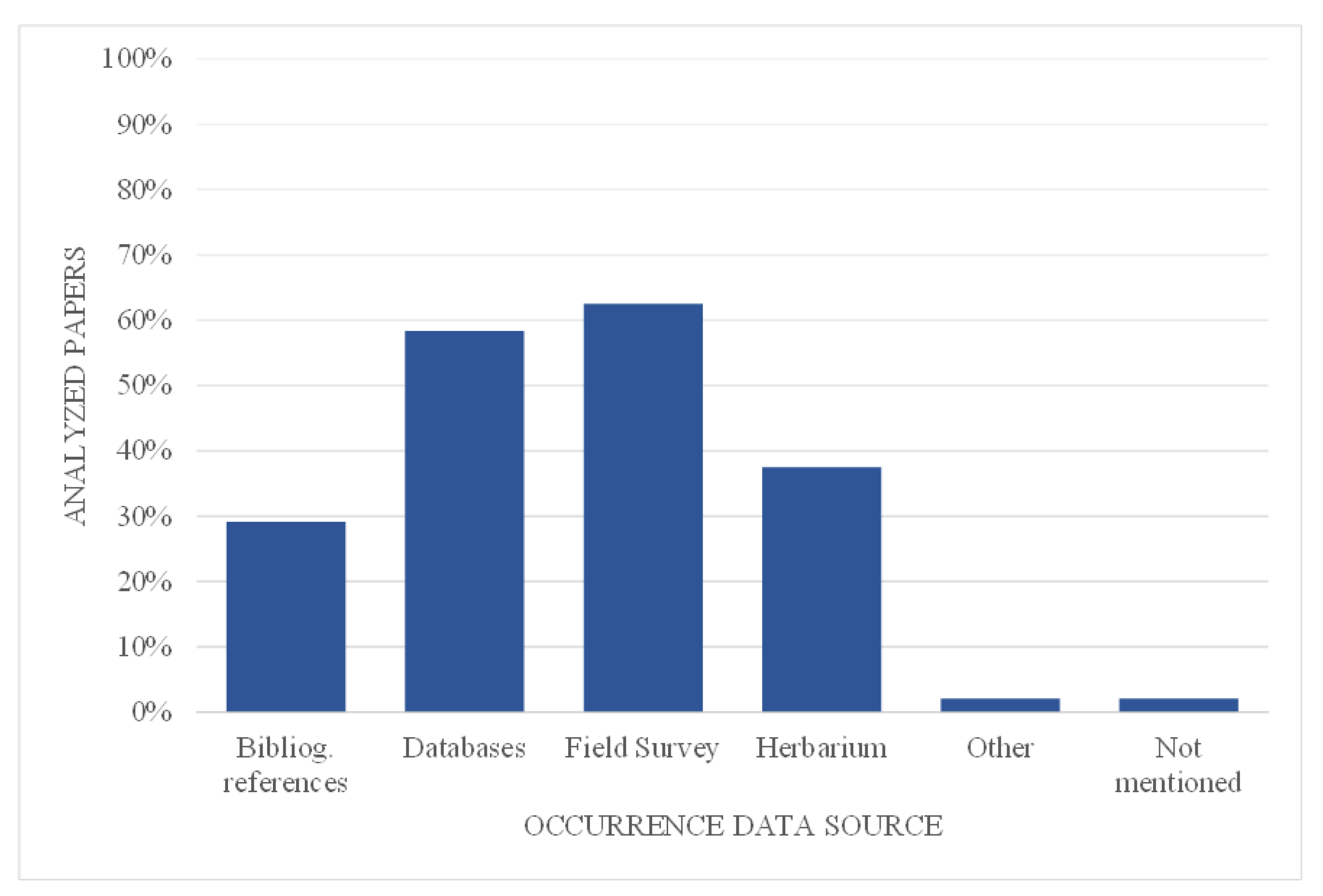
Figure 1. Flow diagram of the selection process, based on PRISMA [80,81].
Preprints 112039 g001
Figure 2. Percentage of analyzed papers considering occurrence data sources.
Preprints 112039 g002
Figure 3. Percentage of papers using other Environmental variables: soil (So), altitude/elevation (Alt/Elev), slope (Sl), hillshade (HS), aspect (Asp), land cover (Lco), populations (Pop), wetland (Wet), distance to (…) (Dist).
Preprints 112039 g003
Figure 4. Accuracy measures used to assess models' performance.
Preprints 112039 g004
Figure 5. Emissions/development scenarios used in analyzed papers: A1b, A2a and B2a from CMIP3 [87]; RCP2.6, RCP4.5, RCP6.0 and RCP8.5 from CMIP5 [88]; SSP126, SSP245, SSP370 and SSP585 from CMIP6 [42].
Preprints 112039 g005
Figure 6. Time windows used in analyzed papers.
Preprints 112039 g006
Table 1. Global Circulation Model (GCM) used in the analyzed studies, and the independent Climate Research Centers (CRC)that developed them. Largest percentages in bold.
Global Circulation Model (GCM) Climate Research Centres (CRC) Country Number of documents by GCM, % Number of documents by CRC, %
ACCESS1-0 Australian Community Climate and Earth System Simulator Coupled Model Australia 2.1 2.1
AFRICLIM York Institute for Tropical Ecosystems (KITE) and Kenya Meteorological Service Kenya 4.3 4.3
BCC-CSM1.1 Beijing Climate Centre Climate System Model China 12.8 25.5
BCC-CSM2-MR 12.8
CanESM5 Canadian Earth System Model Canada 2.1 2.1
CCAFS CCAFS-Climate Statistically Downscaled Delta Method Colombia 6.4 6.4
CCCMA Canadian Centre for Climate Modelling and Analysis Canada 2.1 2.1
CCSM4 National Science Foundation (NSF) and National Centre for Atmospheric Research (NCAR) United States 29.8 31.9
CCSM5 2.1
CGCM3.1-T63 Canadian Centre for Climate Modelling and Analysis Canada 2.1 2.1
CNRM-CM5–1 CNRM (Centre National de Recherches Météorologiques—Groupe d'études de l'Atmosphère Météorologique) and Cerfacs (Centre Européen de Recherche et de Formation Avancée France 2.1 12.8
CNRM-CM6–1 4.3
CNRM-ESM2–1 6.4
CSIRO Commonwealth Scientific and Industrial Research Organisation Australia 2.1 6.4
CSIRO-MK3.6 4.3
GFDL-CM3 Geophysical Fluid Dynamics Laboratory (GFDL) United States 4.3 4.3
GISS-E2-R Goddard Institute for Space Studies (GISS - NASA) United States 2.1 2.1
HadCM3 UK Meteorological Office United Kingdom 2.1 40.4
HadGEM2-AO 4.3
HadGEM2-ES 26.1
HadGEM-CC 4.3
HadGEM-IS 2.1
IPSL-CM5A-LR Institut Pierre-Simon Laplace (IPSL) France 2.1 4.3
IPSL-CM6A-LR 2.1
MIROC5 Center for Climate System Research (CCSR), National Institute for Environmental Studies (NIES); and Japan Agency for Marine-Earth Science and Technology Japan 6.4 14.9
MIROC6 2.1
MIROC-ES2L 4.3
MIROC-ESM 2.1
MPI-ESM-LR Max Planck Institute for Meteorology Germany 2.1 2.1
MRI-CGCM3 Meteorological Research Institute (MRI) Japan 8.5 12.8
MRI-ESM2-0 4.3
NorESM1-M Norwegian Earth System Model (NorESM) Norway 2.1 2.1
Disclaimer/Publisher’s Note: The statements, opinions and data contained in all publications are solely those of the individual author(s) and contributor(s) and not of MDPI and/or the editor(s). MDPI and/or the editor(s) disclaim responsibility for any injury to people or property resulting from any ideas, methods, instructions or products referred to in the content.
Copyright: This open access article is published under a Creative Commons CC BY 4.0 license, which permit the free download, distribution, and reuse, provided that the author and preprint are cited in any reuse.
Prerpints.org logo

Preprints.org is a free preprint server supported by MDPI in Basel, Switzerland.

Subscribe

© 2024 MDPI (Basel, Switzerland) unless otherwise stated