FFA: Foreground Feature Approximation Digitally Against Remote Sensing Object Detection

In recent years, research on adversarial attack techniques for remote sensing object detection (RSOD) has made great progress. Still, most of the research nowadays is on end-to-end attacks, which mainly design adversarial perturbations based on the prediction information of the object detectors (ODs) to achieve the attack. These methods do not discover the common vulnerabilities of the ODs and thus the transferability is weak. Based on this, this paper proposes a foreground feature approximation (FFA) method to generate adversarial examples (AEs) that discover the common vulnerabilities of the ODs by changing the feature information carried by the image itself to implement the attack. Specifically, firstly, the high-quality predictions are filtered as attacked objects using the detector, after which a hybrid image without any target is made, and the hybrid foreground is created based on the attacked targets. The images' shallow features are extracted using the backbone network, and the features of the input foreground are approximated towards the hybrid foreground to implement the attack. In contrast, the model predictions are used to assist in realizing the attack. In addition, we have found the effectiveness of FFA for targeted attacks, and replacing the hybrid foreground with the targeted foreground can realize targeted attacks. Extensive experiments with seven rotating ODs on the RSOD datasets DOTA and UCAS-AOD show that FFA achieves both targetless and targeted attacks with a high success rate and transferability.

Keywords:

Subject: Computer Science and Mathematics - Computer Vision and Graphics

1. Introduction

The development of remote sensing (RS) imaging techniques has led to the advancement of many important applications in RS, including image classification [1,2,3], image segmentation [4,5], object detection [6,7,8], and object tracking [9,10]. Recent studies have found that image-processing techniques based on deep learning exhibit greater potential than traditional image-processing techniques, which makes them a hot research direction and leads to the current implementation of these tasks using deep neural networks (DNNs).

Recent research has demonstrated that DNNs are susceptible to certain perturbations, and the results of detectors can be altered by adding a perturbation to an image that is unrecognizable to the human eye, despite the fact that deep learning has achieved increased success [11,12]. This phenomenon reveals the great security risks of DNNs and also inspires people to research their security. Adversarial examples (AEs), which can be created by subtly altering the source image to increase the success rate of attacks, were initially identified by Szegedy et al. [13]. Since then, more and more people have been devoted to studying the vulnerabilities of DNNs and improving their security and robustness.

Object detection [14], as an important research area in image processing, has likewise given birth to some important applications, such as autonomous driving [15,16] and intelligent recognition systems [17,18], and naturally has yet to escape the attack of AEs. Compared with attacking image classification, attacking object detection is more difficult [19]. In image classification, each image contains only one category, which is easier to realize. In object detection, in which each image contains multiple objects, it is necessary to find out the object as well as determine its location and lock its size, which leads to object detection being more practical but more difficult to attack. Therefore, it is more meaningful to attack the object detection system and study its vulnerabilities.

Adversarial attacks can be classified into digital and physical attacks, depending on the domains in which they are applied [19]. Digital attacks mainly make the detector detect errors by changing the image pixels, which is applicable to all images, such as the DFool attack proposed by Lu et al. [20] and the DAG attack proposed by Xie et al. [21]. Physical attacks mainly make the detector misclassify by adding patches to the objects, mainly for images with a large percentage of objects. Kurakin et al. [22] first experimentally verified that AEs are also present in the actual world, and Thys et al. [23] successfully spoofed a pedestrian monitor by generating adversarial patches.

Remote sensing images (RSI), with their high resolution and wide spatial distribution, add some difficulties for object detection and likewise lead to their difficulty in realizing physical attacks [24,25]. Therefore, the majority of the current attacks on RSI are digital attacks, and a few physical attacks are limited to RSI with a large percentage of targets. Czaja et al. [24] first investigated the AEs in RSI and successfully attacked the image classification models. Lu et al. [25] successfully designed an adaptive patch to attack the object detectors (ODs) for RSI. Du et al. [26] and Lian et al. [27] successfully applied adversarial patches against RSI to the physical world. More and more people have been devoted to the work of RS adversarial attacks.

The work of Xu et al. [3] and Li et al. [19] inspires us. Xu et al. [3] investigated the generic AEs for RSI classification models, and Li et al. [19] devised a method for adaptively controlling the perturbation size and location based on the behaviour of the ODs. It is well known that object detection has three main tasks: determining the object location, determining the object size, and determining the object category [14]. These are indispensable, and the attack can be realized by successfully attacking any one of the three tasks. Determining the object category is the image classification task, so we choose to attack the classifier in the ODs. We found that for object detection, using global adversarial perturbation will result in a significant resource waste since the objects in the RSI only represent a minor fraction of the entire image, and the background accounts for a much larger portion than the foreground, so we use local adversarial perturbation, which only changes the pixels in the foreground portion.

We suggest a digital attack method in this paper, which we call Foreground Feature Approximation (FFA), which mainly utilizes the backbone network of the ODs (feature extraction network) to attack the classifier. As an important part of the detection task and is most effective in utilizing it for the attack. The attack effect of FFA is shown in Figure 1.

The contributions of this paper are as follows:

We propose the FFA attack, which uses the high-quality prediction of the ODs as the foreground, extracts shallow features using the ODs’ backbone network, and approximates the features of the input foreground image towards the features of the hybrid foreground image only by changing the pixels in the foreground part of the image, which achieves the targetless attack;
We replaced the hybrid image with an image of the specific class, constructed the target foreground based on the high-quality prediction of the ODs, extracted the shallow features of the target foreground using the backbone network as well, and later approximated the input foreground features towards the target foreground features to achieve the targeted attack;
The results of attacks on seven rotating ODs on the RSOD datasets DOTA and UCAS-AOD demonstrate that our method can produce AEs with higher attack capability, higher transferability, and higher imperceptibility.

2. Related Work

We touch on the theory of adversarial attacks in this section, including those used in image classification, object detection and RS.

2.1. Adversarial Attacks in Image Classification

Image classification is a critical task in machine learning, the goal of which is to enable the computer to assign input images to the real categories [28]. Given an input image

x

, whose true label is y, and the model’s prediction function is

f (\cdot)

. The task of correctly classifying the image is even if the model’s prediction is equal to the true label of the target, that is

f (x) = y

. Generating AEs

x^{'}

for an image classification model requires generating an adversarial perturbation

δ

, then

x^{'} = x + δ

. By limiting the size of the perturbation, it is possible to generate AEs that appear unchanged to the human eyes but that the computer cannot correctly classify, even if

f (x^{'}) \neq y

. The above method is an targetless attack, which only requires that the computer be rendered incapable of correct classification. Adversarial examples also enable targeted attacks, also known as directed attacks, where the goal is to make the computer assign our carefully designed AEs to a particular class, assuming that the label of the particular class is p, and

f (x^{'}) = p \neq y

In the beginning, people studied white-box attacks [29,30,31]. This method assumes that the structure and parameters of the models we want to attack are known, and when we attack according to this known information, the attack success rate of these methods is higher. For example, the optimization-based method L-BFGS [13] and gradient-based method FGSM [32] are white-box attack methods. However, in practice, it is difficult to get the framework and settings for the target models, so black-box attacks arise [33]. A black-box attack assumes that the framework and settings for the target models are unknown, and we need to discover the vulnerability of the target models through the known models and other information to realize the attack. The attack success rate of this method is generally low but has a high value of use. For example, transfer-based attacks Curls&Whey [33], FA [2], etc., query-based attacks ZOO [34], MCG [35], etc. and decision boundary-based attacks BoundaryAttack [36], CGBA [37], etc. are black box attack methods.

2.2. Adversarial Attacks in Object Detection

Object detection, an advanced task of image classification and segmentation, occupies an increasing share in computer vision and is also applied in task scenarios such as face recognition [38], unmanned vehicles [39], aircraft recognition [40], terrain detection [41], etc. The goal is for the computer to find the part of interest in an image and give it the correct classification, location, and size. The emergence of AEs also puts higher demands on the security of object detection.

Xie et al. [21] first discovered the existence of AEs in object detection and semantic segmentation tasks. They proposed the DAG attack with good transferability between multiple datasets and different network structures. The target of the attack is placed in the region of interest (RoI), and the attack expression is:

δ_{m} = \sum_{t_{n} \in T_{m}} [\nabla_{X_{m}} f_{l_{n}^{'}} (X_{m}, t_{n}) - \nabla_{X_{m}} f_{l_{n}} (X_{m}, t_{n})],

(1)

x_{m + 1} = x_{m} + \frac{α}{{∥δ_{m}∥}_{\infty}} δ_{m},

(2)

where

δ_{m}

denotes the perturbation generated by the mth iteration,

x_{m}

denotes the AE generated by the mth iteration.

t_{n}

denotes a certain object among all objects

T_{m}

in the image,

f (\cdot)

denotes the result function of object detection,

l_{n}

refers to the true category label of the attacked object, and

l_{n}^{'}

refers to the category label specified by the attack. The perturbation is also normalized in order to limit the range of the perturbation.

α

denotes the iterative learning rate, which controls the range of the perturbation and is a fixed hyperparameter value.

Lu et al. [20] proposed the DFool attack to construct AEs against intersection stop signs in videos to successfully attack the then more advanced Faster RCNN [42] model and implement the attack in the physical world as well. It generates AEs by minimizing the average score produced by Faster RCNN for all stop signs in the training set. The average score of stop signs is:

Φ (T) = \frac{1}{N} \sum_{i = 1}^{N} b \in B_{s} (I^{m e a n} (M_{i}, T)) Φ_{s} (b),

(3)

where

T

denotes the texture of the stop sign in the root coordinate system,

I (M_{i}, T)

denotes the image

I

formed using the mapping

M_{i}

superimposed on the

T

M_{i}

is the mapping formed by the correspondence between the eight vertices of the stop sign and the vertices of the

T

B_{s} (I)

is the set of stop signs detected by the image

I

through the Faster RCNN, b is a certain detection box, and

Φ_{s} (b)

denotes the score predicted by the Faster RCNN for the detection box.

Afterwards a small gradient descent direction is used for optimization:

δ^{(n)} = sign (\nabla_{T} Φ (T^{(n)})),

(4)

T^{(n + 1)} = T^{(n)} + ε δ^{(n)},

(5)

where sign(·) denotes the sign function, which is used to control the size of the perturbation,

T^{(n + 1)}

denotes the AE generated by the n+1st iteration.

ε

denotes the iteration step size and

δ^{(n)}

denotes the adversarial perturbation generated by the nth iteration.

Both of the above methods are global perturbation attacks [3,43], i.e., each pixel in the image is changed to generate the AE. The defects of these methods are very obvious. They change the foreground and background at the same time, resulting in a waste of attack resources and prolonging the attack time. Based on this, researchers have discovered local perturbation attacks [19,44] and gradually developed them as patch attacks [23,27] in the physical world.

The Dpatch attack was put forward by Liu et al. [45], which centres on generating a patch with the ground truth detection box property and optimizing it into a real object through backpropagation. In addition, the OD is made to ignore other possible objects. For two-stage ODs, such as Faster RCNN [42], the idea of the attack is to make the RPN network unable to generate the correct candidate network so that the generated patch becomes the only object. For single-stage ODs, such as YOLO [46], the core of which is the bounding box prediction and confidence scores, the attack is to make the grid where the patch is located be regarded as an object and ignore other grids. The objective function is optimized by training the patches, and the resulting patches are:

\hat{p} = arg max_{p} E_{x, t, l} [log P (\hat{y} | A (p, x, l, t))],

(6)

where

A (p, x, l, t)

represents that the input image

x

places the patch

p

on l through a transformation t, the transformation t includes basic transformations such as rotation scaling.

P (\hat{y} | A)

represents the likelihood that the input

A

is associated with the label

\hat{y}

. The principle of Dpatch is to maximize the loss of the ODs to the true label and the bounding box label.

Thys et al. [23] designed the first printable adversarial patch for pedestrians, which achieved better attack results against the YOLO V2 OD in the physical world. Their optimization objective consists of three parts.

One is the non-printable score

L_{n p s}

, which donates whether the patch can be printed using a printer:

L_{n p s} = \sum_{p_{patch} \in P} min_{c_{print} \in C} |p_{patch} - c_{print}| L_{n p s},

(7)

let

p_{patch}

represent a pixel in P, and

c_{print}

represent a colour in a set of printable colours in C. This loss benefits colors in the image that closely resemble the colors in the set of printable colors.

The second is the total cost

L_{t v}

in the image, which is used to ensure a smoother transition between the patch and the image:

L_{t v} = \sum_{m, n} \sqrt{{(p_{m, n} - p_{m + 1, n})}^{2} + {(p_{m, n} - p_{m, n + 1})}^{2}},

(8)

The third is the maximum objective score

L_{o b j}

of the image, which represents the score assigned to the object detected by the detector. The three are combined according to reasonable weights, and adversarial patches are generated iteratively.

2.3. Adversarial Attacks in Remote Sensing

Adversarial attacks have been investigated in ground imagery but they also have numerous uses in RS. Li et al. [19] designed an adaptive local perturbation attack method aiming at generalizing the attack to all ODs, which establishes an object constraint to adaptively utilize foreground-background separation to induce perturbations as a way of controlling the magnitude and distribution of perturbations so that perturbations are attached to the object region of the image. It employs three loss functions: classification loss, position loss, and shape loss, to generate the AE, and the three parts of the loss are rationally combined using a weighted approach.

L = \sum_{n = 1}^{N} α L_{s h a p e} (b_{n}, b_{n}^{'}) / N + \sum_{n = 1}^{N} β L_{l o c} (b_{n}, b_{n}^{g t}) / N + \sum_{n = 1}^{N} τ L_{c l s} (p_{n}, ℓ_{b}),

(9)

where N denotes objects’ number in the image,

L_{s h a p e}

denotes the shape constraint,

L_{l o c}

denotes the location constraint,

L_{c l s}

denotes the classification constraint, and

α, β, τ

refers to the weights of the three constraints. Each object is assigned a random bounding box

b_{n}^{'}

for shape attack, a real border

b_{n}^{g t}

for localization attack and a background category

ℓ_{b}

for classification attack. In addition, the distribution of perturbations is adaptively controlled using the foreground separation method so that the perturbations are attached to the foreground as much as possible.

Lian et al. [27] investigated physical attacks in RS. They proposed the patch-based Contextual Background Attack (CBA), which aims to achieve steganography of the object in the detector without contaminating the object in the image. It places the patch outside the object instead of on the object, which is more conducive to the realization of physical attacks. An AE with an adversarial patch can be precisely described as:

x_{a d v} = (1 - M_{p^{*}}) ⊙ x + M_{p^{*}} ⊙ P^{*},

(10)

where

P^{*}

denotes the antipatch,

M_{p^{*}}

denotes the mask of the antipatch, foreground pixels are 1 and background is 0, and ⊙ denotes the Hadamard product.

Objectivity loss and smoothness shrinkage are also used to update the adversarial patches. Objectivity loss refers to updating the AEs by detecting differences between objects in the inner and outer parts of the patch, and smoothing contraction reduces the distance between the patch and the target to make the transition smoother.

3. Methodology

3.1. Problem Analysis

To design a compliant AE, two aspects need to be considered (1) where the perturbation is placed; (2) how the perturbation should be designed.

3.1.1. Location of the Perturbations

To enhance the effectiveness of the perturbation, we need to choose a suitable location to add the perturbation. Compared with the global adversarial perturbation for the image classification task, it is not very suitable to design a global adversarial perturbation for the object detection task. Especially for RSI object detection, the number of objects is large, and the area occupied is small. In this case, we need to design a more useful perturbation generation strategy to limit the perturbation to a suitable range.

3.1.2. Magnitude of the Perturbations

After determining the location of the perturbation, the next step is to determine its design scheme. The principle of perturbation generation is to successfully deceive the ODs and ensure that human eyes cannot perceive them. Therefore, the design of the perturbation can be seen as a joint optimization problem by considering multiple factors and balancing multiple losses so that the final generated AEs are globally optimal rather than locally optimal.

The input picture is expected to be

x

and there are n objects in the image.

{B^{i}}_{n} = (w_{n}, h_{n}, x_{n}, y_{n}, l_{n}, s_{n})

is the parameter of the ith object, which represents the width, height, centroid horizontal coordinate, centroid vertical coordinate, object label, and object score of the object box, respectively. When detecting rotated objects, the object box’s rotation angle parameter must be added. The goal of AE design is to identify an appropriate perturbation

δ

that satisfies:

arg min_{δ} P^{i} (x + δ) \neq {B^{i}}_{n},

(11)

where P denotes the detector,

P^{i} (x + δ)

represents the image’s ith detection result, and the generated AE is

x + δ

. It can be seen from this that there are three manifestations of a successful attack: first, the size of the detection box is incorrect; second, the location of the detection box is incorrect (including no detection box, i.e., the object is "invisible" in the detector), and third, the category of the detected object is incorrect. These three manifestations can be superimposed.

3.2. Overview of the Methodology

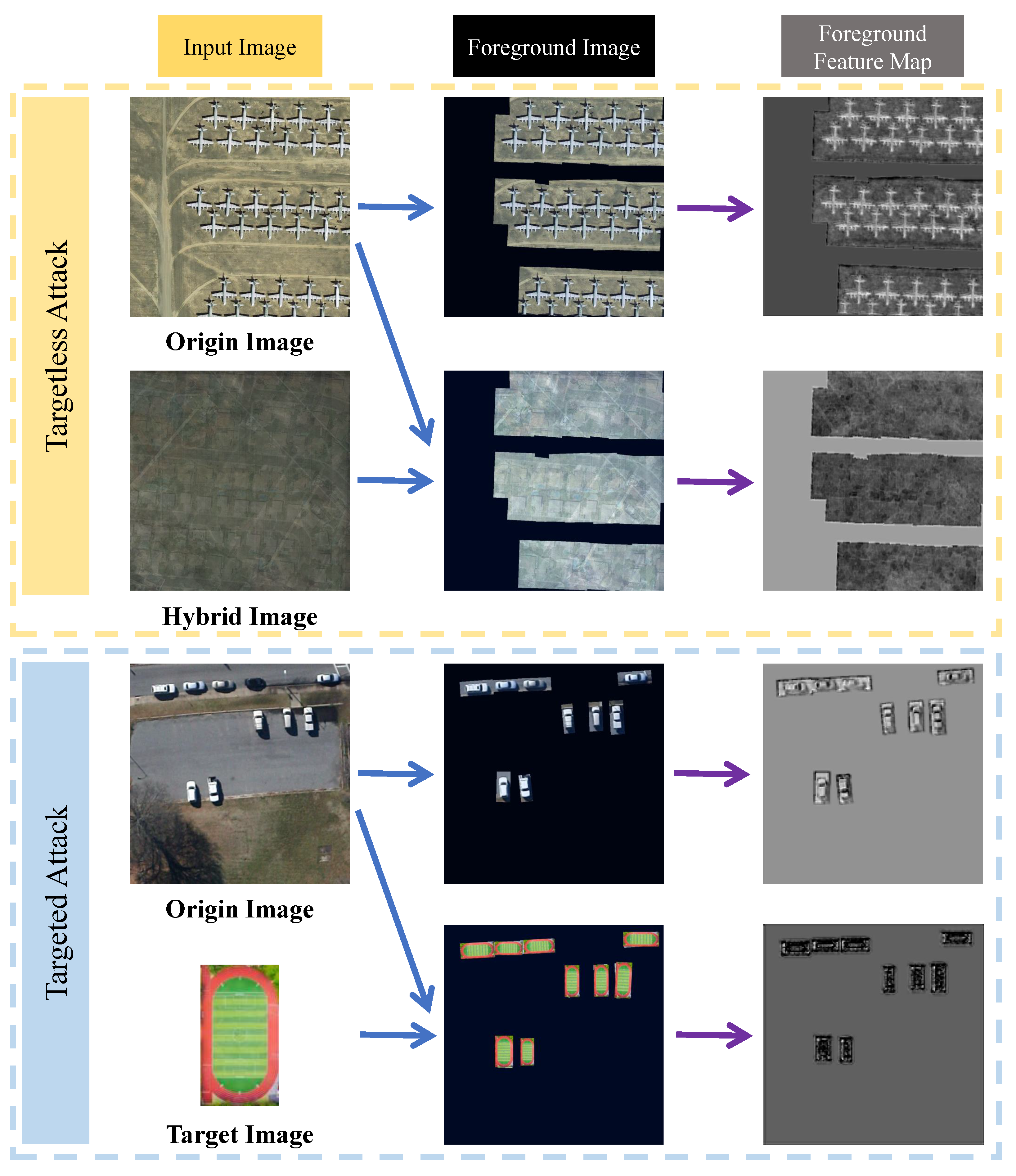
The topic of attacks against ODs has been extensively studied. Since ODs contain several important components, attacks against these specific components are effective. Still, they also pose a huge problem at the same time: specific ODs contain specific frameworks and components, which prevent the generalization of the attacks [19]. In order to improve the transferability of attacks, we need to discover the similarities between different ODs. All ODs are inseparable from a common backbone network. The most commonly used backbone network is the ResNet network [8]. So we can change the features of the image for the attack and can form an AE with high transferability. The process of extracting features is visually represented in Figure 2.

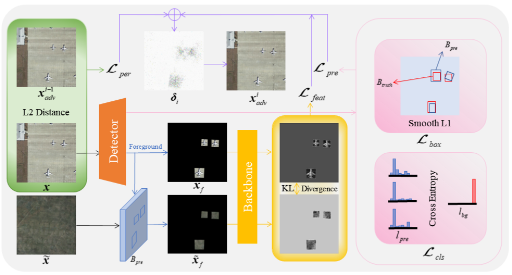
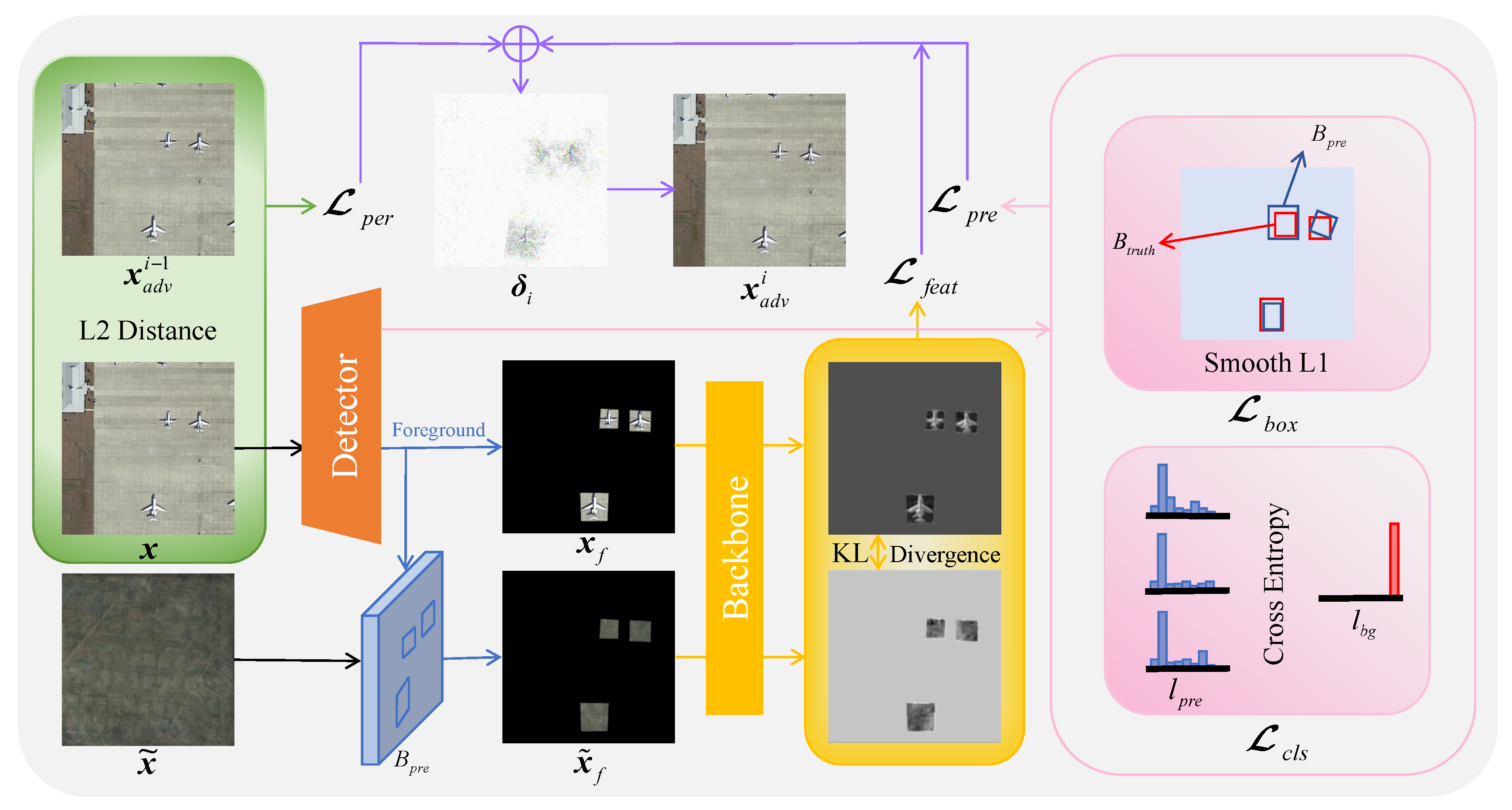
We first use an OD to detect the image, separate the high-quality foreground and the background, make a record of the foreground data of the image, including the object category as well as the position and the object box size, and cut the image of all the object boxes as a backup. After that, we need to design a hybrid image with the principle that it can’t contain objects of either category, and its dimensions are identical to those of the original image. Utilize the backbone network for obtaining the features of hybrid foreground and high-quality foreground, design the body of the loss function by minimizing the KL-divergence between the latter and the former, and use the prediction result of the OD to perform the assisted attack. To accomplish the attack, the original image’s pixels should finally be altered so that the hybrid image’s features roughly match those of the original image. The flowchart of FFA attack is shown in Figure 3.

3.3. Foreground Feature Approximation (FFA) Attack

3.3.1. Targetless Attack

1. Location of the perturbation

For the object detection task, only the foreground section of the image, which is a small part, is relevant, while the background portion is irrelevant. Therefore, to attack the object detection, we only need to add perturbations to the portion of the ODs that is of interest. We use the attacked ODs to predict the image, get the prediction boxes and perform further filtering based on the prediction boxes scores:

T_{b b o x e s} = \{\begin{matrix} P_{b b o x e s} (x), & s c o r e s_{m a x} > α \\ 0, & s c o r e s_{m a x} < α \end{matrix} (0 < α < 1),

(12)

where

T_{b b o x e s}

is the object to be attacked,

P_{b b o x e s}

is the prediction boxes of the ODs,

s c o r e s_{m a x}

is the maximum value of the prediction scores for each category,

α

is the threshold of the prediction scores, the prediction boxes with prediction scores greater than

α

are selected as the object to be attacked, and the prediction boxes with prediction scores less than

α

are considered to have no value to be attacked, and we do not attack them.

2.The size of the perturbation

Most of the previous methods design perturbations based on the predictive information of ODs and construct a variety of loss functions based on the object boxes detected by the ODs as well as the object categories, including position loss, shape loss, category loss, and so on. These methods depend on the accuracy of the ODs and the fact that the generated AEs do not have high transferability. Based on this, we propose a feature approximation strategy to change the features of the image in the view of the backbone network to mislead the detectors and achieve the attack effect. The loss function is designed as follows.

Feature Loss: After selecting the foreground portion to attack, we need to design a suitable loss function to update the perturbation iteratively. Before starting, we need to generate a hybrid image

\tilde{x}

to determine the direction of each iterative update. We choose ten images from the training set of the dataset to be superimposed, and the final image formed by the superimposition is a hybrid image that does not contain any object, which we call the full background image.

Using the prediction boxes obtained from the ODs, the input image

x_{a d v}^{i}

and the hybrid image

\tilde{x}

of the ith iteration are cropped separately to obtain the input foreground

x_{a d v_f}^{i}

and the corresponding hybrid image

{\tilde{x}}_{f}

. We define the feature loss function as the KL-divergence between the two images’ pixel distributions:

L_{f e a t} (θ, x_{a d v_f}^{i}, {\tilde{x}}_{f}) = - \sum_{R = 1}^{N_{R}} \sum_{C = 1}^{N_{C}} \sum_{K = 1}^{N_{K}} f_{θ} {(x_{a d v_f}^{i})}^{(R, C, K)} l o g \frac{f_{θ} {(x_{a d v_f}^{i})}^{(R, C, K)}}{f_{θ} {({\tilde{x}}_{f})}^{(R, C, K)}},

(13)

where

L_{f e a t}

denotes the feature loss,

θ

denotes the backbone network parameters, and

N_{R}, N_{C}, N_{K}

denotes the number of rows, columns, and channels of the feature map, respectively.

f_{θ} (\cdot)

denotes the mapping function for extracting shallow features using the backbone network. Note that the formula is preceded by a negative sign in order to minimize the KL-divergence of the clean and mixed foregrounds.

To improve the effectiveness of the attack, we also have to design the prediction loss to assist the attack based on the ODs’ prediction results. The classification loss and the object box loss are the two components of this loss.

Classification Loss: Let the AEs carry incorrect labelling information to mislead the classifier. Since the probability that the predicted object is background is calculated during the detector prediction process, it has a background label, which we assume to be

l_{b g}

. Assume that the prediction results in m objects

x_{0}, x_{1}, \dots x_{m - 1}

. Their labels are finding the true label of a prediction box by calculating the cross-entropy loss of the true box to the prediction box. By reducing the cross-entropy loss between the background category and the prediction box category, the attack is accomplished. The classification loss for each object is:

{L^{j}}_{c l s} (x_{j}, l_{b g}) = \sum_{C = 1}^{N_{L}} {l_{b g}}^{(C)} l o g P {(x_{j})}^{(C)},

(14)

where

N_{L}

indicates the number of categories in all images,

P (\cdot)

is the mapping function of the ODs’ detection results,

x_{j}

is the jth object, and the total classification loss for this image is:

L_{c l s} (x, l_{b g}) = \sum_{j = 1}^{m} L_{c l s}^{j} (x_{j}, l_{b g}),

(15)

Object box loss: this loss is used to control the offset between the real object box and the prediction box. By increasing this offset, the gap between the detection result and the real result gets bigger and bigger to carry out the attack. Assuming that the centroid of the jth prediction box has the coordinates

O_{j} = (h_{j}, v_{j})

, and the centroid of the real box corresponding to this prediction box has the coordinates

O = (h, v)

, the Euclidean distance

D_{j}

between the two is calculated, and the object box loss is defined in terms of the Smooth L1 loss at this distance:

{L^{j}}_{b o x} = S L 1 (D_{j}) = \{\begin{matrix} 0.5 D_{j}^{2}, & D_{j} < 1.0 \\ D_{j} - 0.5, & o t h e r w i s e \end{matrix},

(16)

The object box loss for the entire image is then the sum of the object box losses for each prediction box:

L_{b o x} = \sum_{j = 1}^{m} {L^{j}}_{b o x} (D_{j}),

(17)

The prediction loss is the sum of the categorization loss and the object box loss, both of which are equally weighted:

L_{p r e} = L_{c l s} + L_{b o x},

(18)

Perceptual Loss: In order to make the perturbation look more natural, we also need to control the range of the perturbation. The perceptibility of the AEs is reduced by minimizing the L2 distance between the AEs and the original images. Assuming that the ith iteration generates an adversarial example

x_{a d v}^{i}

, we define the perceptual loss as:

{L^{i}}_{p e r} = {∥x_{a d v}^{i} - x∥}_{2},

(19)

The ultimate loss function is a weighted combination of the three losses:

L = L_{f e a t} + β L_{p r e} + γ L_{p e r},

(20)

The AE generated in the ith iteration is:

x_{a d v}^{i} = x_{a d v}^{i - 1} + \nabla_{x} L^{i},

(21)

where

\nabla_{x} L^{i}

denotes the gradient of the computational loss

L^{i}

with respect to the original image

x

Algorithm 1 gives the implementation details of the FFA to achieve the targetless attack.

Algorithm 1: Foreground Feature Approximation (FFA).

Input:
-Input image $x$ and its ground truth $B_{n}$ ;
-A object detector D with the prediction function $P (\cdot)$ and the feature extraction
function $f (\cdot)$ ;
-Hybrid image $\tilde{x}$ .
Initialization:
1. $x_{a d v}^{0} \leftarrow x, I \leftarrow 50, α \leftarrow 0.75, β \leftarrow 0.1 γ \leftarrow 0.1 .$
2. $T_{b b o x e s} \leftarrow P^{D} {(x) |}_{s c o r e s_{m a x} > a}$
Iteration:
for t in $r a n g e (0, I)$ do
1. $x_{a d v_f}^{i} \leftarrow T_{b b o x e s} (x_{a d v}^{i}), {\tilde{x}}_{f} \leftarrow T_{b b o x e s} (\tilde{x})$
2. $L^{i} \leftarrow Combine {L_{f e a t}^{i}, L_{p r e}^{i}, L_{p e r}^{i}}$
3. $x_{a d v}^{i} \leftarrow U p d a t e {x_{a d v}^{i - 1}, L^{i}}$
end for
return $x_{a d v}^{I}$

3.3.2. Targeted Attack

1. Location of the perturbation

As with the targetless attack, we use Equation (12) to obtain the objects

T_{b b o x e s}

of the attack.

2.The size of the perturbation

The targeted attack is executed by deceiving the classifier in the detector, causing it to classify all of the objects in the image as the specific target. The loss function is designed as follows.

Feature Loss: To realize the targeted attack, we use an image of the target category instead of the original hybrid image and extract a target in the target image as a benchmark. Due to the large number of prediction boxes and their different sizes, we have to redesign the target foreground before performing feature approximation. First, create a blank image that is the same shape as the input image, identify the location and size of each prediction box, and resize the target image so that the two are of the same size, following which the target image is transferred into the corresponding position in the blank image to create a new target foreground

{\tilde{x}}_{f_t}

. After that, the feature loss is computed:

L_{f e a t_t} = L_{f e a t} (θ, x_{a d v_f}^{i}, {\tilde{x}}_{f_t}),

(22)

Classification Loss: The design principle of targeted attack is to move the classification result of the classifier continuously closer to the target label, assuming that the target label is

l_{t}

. The classification loss is calculated as follows:

L_{c l s_t} = L_{c l s} (x, l_{t}),

(23)

Object box loss: in contrast to targetless attacks, the object box loss in targeted attacks is designed to allow the detection box to coincide with the real box gradually, and thus, the loss is designed to be:

L_{b o x_t} = - \sum_{j = 1}^{m} {L^{j}}_{b o x} (D_{j}),

(24)

As with the targetless attack, the total of the object box loss and the classification loss is the prediction loss.

Perceptual Loss: As with the targetless attack, we construct the perceptual loss by minimizing the L2 distance between the clean image and the AE.

The ultimate loss function is a weighted amalgamation of the three loss functions. The adversarial perturbation is determined by calculating the gradient of the loss function in relation to the input image. Adding the perturbation to the input image creates the AE.

4. Experiments

4.1. Experimental Preparation

4.1.1. Datasets

We examine our method on two frequently used RSOD datasets, DOTA [47] and UCAS-AOD [48].

DOTA [47]: Since the original images of this dataset are too large, we cropped the original dataset to facilitate the processing. The whole dataset has more than 5000 PNG images with 1024×1024 pixels after cropping. After our filtering, we get 1500 images covering 15 categories. This research utilizes the DOTA dataset to validate the efficacy of FFA in targetless attacks.

UCAS-AOD [48]: This dataset contains a total of 1,510 images and 14,596 image instances of only two categories, aircraft and vehicles. The counterexample images in the dataset are of less value for the study of adversarial attacks, and thus, we do not consider them. As with the DOTA dataset, we cut the images and processed them to contain a total of 3000 plane images and 1,500 vrhicle images, each with pixels of 680×680. We filter the dataset finely and remove similar images to obtain 1,000 aeroplane images and 1000 car images, which constitute our experimental dataset. This dataset is used to validate the performance of FFA with targeted attack.

4.1.2. Detectors

In total, we selected seven rotated ODs as both training and attacked detectors, four for two-stage detectors, namely Oriented R-CNN (OR) [49], Gliding Vertex (GV) [50], RoI Transformer (RT) [51], and ReDet (RD) [52], and three in total for single-stage detectors, namely Rotated Retinanet (RR) [53], Rotated FCOS (RF) [54] and S2A-Net (S2A) [55]. For the feature extraction network, we use ResNet50 [8], hereafter referred to as R50. All the above models are implemented using the open-source MMrotate [56] toolbox.

4.1.3. Evaluation Metrics

For targetless attacks, we use the mean accuracy (mAP) to evaluate the attack effect of the FFA attack. As long as the detected object class is not a real class, the attack is judged to be successful. The smaller the mAP, the better the attack effect is. For targetless attacks, we use mAP and the number of detection boxes

N_{t}

of the target class detected by the detector to validate the effect of the attack. The smaller the mAP, the bigger the

N_{t}

indicates that the effect of the attack is better. The IoU threshold is set to 0.5. For image perceptibility, we use Information content weighted Structural SIMilarity (IW-SSIM) [57] to evaluate the AEs’ perceptibility. The smaller the value, the lower the perceptibility of the image perturbation and the better the effect. For observational comparison, we multiply both mAP50 and IW-SSIM data by 100. In addition, we assess the attack speed of various algorithms by calculating the average attack time of an image computed using an NVIDIA GeForce RTX 3060 (12GB) graphics card.

4.1.4. Parameter Setting

The iterations number I is set to 50, the learning rate is assigned a value of 0.1, and the threshold for high-quality prediction box filtering

α

is set to 0.75. For the targetless attack, the weight of feature loss is set to 1, and the weights

β

and

γ

of prediction loss and perceptual loss are set to 0.1. For the targetless attack, the weight of prediction loss

β

is set to 1, and that of perceptual loss

γ

is set to 0.1.

This study was implemented on the Pytorch platform.

4.2. Targetless Attack

The test of targetless attack is performed on the DOTA [47] dataset using seven rotating ODs, whose backbone networks are all ResNet50 [8]. We test the attack capability of the attacks using the mAP with an IoU threshold of 0.5 (hereafter referred to as

{mAP}_{50}

), with smaller values indicating stronger attack capability. We test the imperceptibility of the perturbation using IW-SSIM [57], with smaller values indicating that the perturbation is imperceptible. We use the average attack time of each image to test the attack speed of all attacks; the smaller the value, the faster the attack speed. Table 1 illustrates the experimental outcomes. In order to facilitate the observation, we multiply the value of

{mAP}_{50}

with the value of IW-SSIM by 100 to get the data in the table.

From the data in the table, we can see that the attack capability of FFA is significantly stronger than the current state-of-the-art methods, especially since the attack transferability obtains a large improvement. The reason is that we designed a generic attack for the current commonly used backbone network by changing the characteristics of the image in the view of the backbone network, attacking the model’s attentional mechanism. Thus generating the adversarial perturbation with a more powerful attack. The imperceptibility of the perturbation generated by FFA is slightly weaker than the LGP attack due to the fact that LGP designs an adaptive perturbation region updating strategy to select more cost-effective regions to attack. On the other hand, FFA selects the attacked regions based on the prediction of the ODs and the real labels of the clean images, which implies that the ODs’ detection accuracy and the attacking effect of FFA are somewhat correlated, and it will inevitably select some cost-ineffective regions for attacking during the attacking process, which attenuates the imperceptibility of the perturbation. In terms of attack speed, FFA is slightly slower than LGP because FFA uses the feature approximation strategy, and the feature distance has to be calculated during the attack process, which increases the amount of computation. FFA sacrifices part of the imperceptibility and attack speed for the improvement of attack effectiveness.

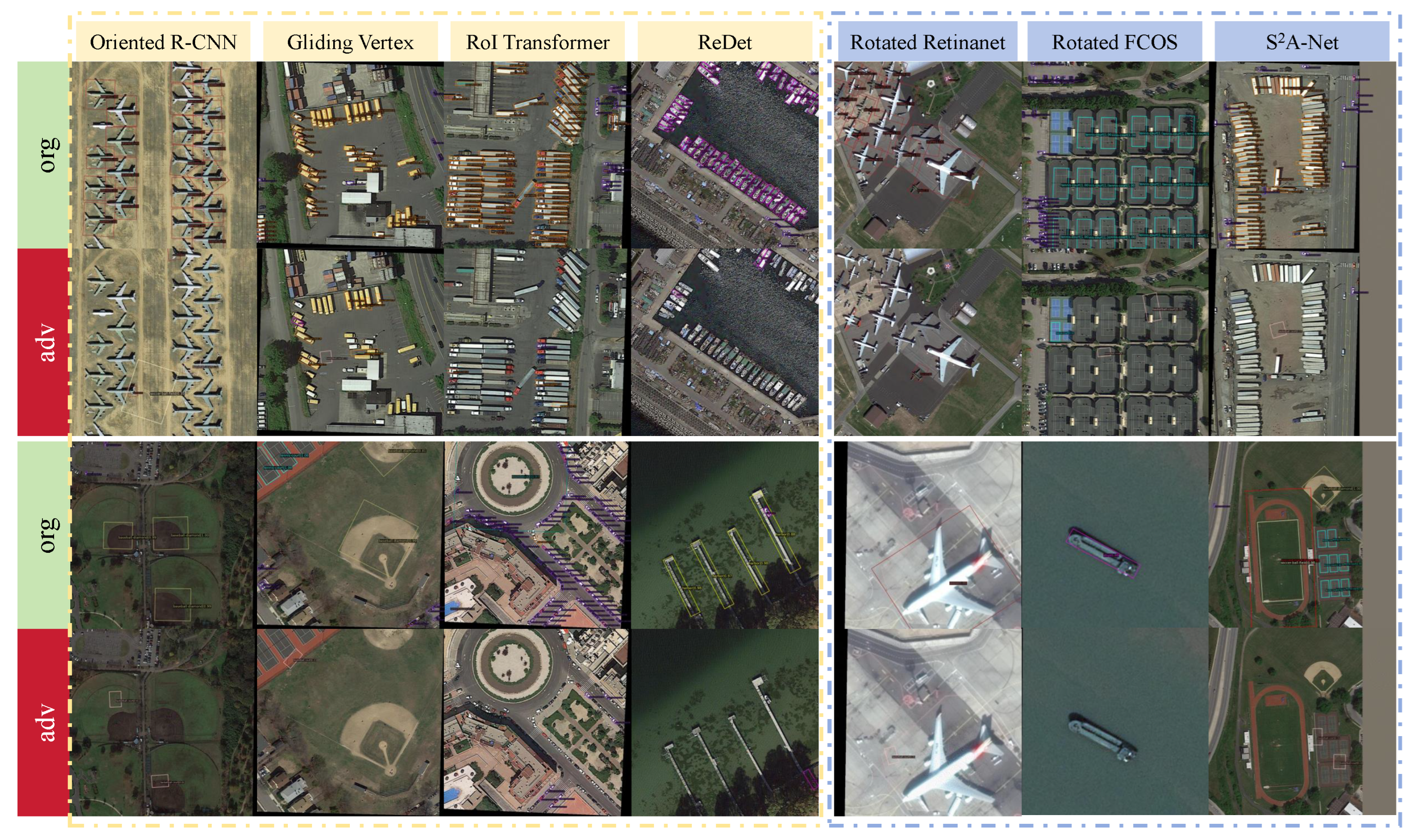
The visualization results of the targetless attack are displayed in Figure 4. Based on the figure, it is evident that the FFA produces better attack results not only for large and sparse objects but also for small and dense objects.

4.3. Targeted Attack

4.3.1. White Box Attack Performance

Targeted attacks were tested on the UCAS-AOD [48] dataset using seven rotating ODs whose backbone networks are all ResNet50. We tested the method’s attack capability using

{mAP}_{50}

and the number of targets

N_{t}

with the IoU threshold of 0.75 (hereafter referred to as

N_{t 0.75}

), where a smaller value of

{mAP}_{50}

and a larger value of

{mAP}_{50}

indicate a stronger attack capability. The test results are shown in Table 2. From the table, it can be seen that FFA’s attack capability is significantly stronger than the existing advanced attack methods. This shows that FFA can realize a high success rate by changing the object features in the image.

4.3.2. Transferability Experiments

To verify the targeted attack transferability of FFA, we designed the following experiment. A two-stage OD OR [49] and a single-stage OR S2A [55] are selected as trained detectors to attack the remaining five detectors, with the original categories of planes and vehicles and the corresponding target categories of basketball courts and ground track fields, respectively. The evaluation metrics are

{mAP}_{50}

and

N_{t 0.75}

. The empirical findings are displayed in the Table 3.

The data presented in the table demonstrates that FFA has better transferability compared to other methods. We also find that FFA has a stronger attack effect on simple models than on complex models.

{mAP}_{50}

of FFA for single-stage detectors is, on average, 2 percentage points lower than that of dual-stage detectors, while

N_{t 0.75}

is, on average, more than 200. In addition, the accuracy of the trained OD also affects the attack effect. Since the accuracy of the two-stage OD is slightly higher than that of the single-stage OD, the attack effect of the attack using the two-stage OD is stronger than that using the single-stage OD. At the same time, the success rate of targeted attacks on planes is significantly higher than that of vehicles because the ODs’ detection accuracy for planes is higher than that of vehicles.

4.3.3. Imperceptibility and Attack Speed Test

Similar to the targetless attack, we also tested the perturbation’s imperceptibility and the algorithm’s attack speed. The empirical findings are displayed in the Table 4.

The data presented in the table demonstrates that the perturbation imperceptibility type of FFA is slightly weaker, and the attack speed is slower than LGP. The reason is that we will sacrifice some of the perturbation imperceptibility with the attack speed to get a high-transferability attack. In addition, we also find that the success rate of attack against single-stage ODs is higher than that of two-stage ODs due to the simpler model structure and longer attack time of single-stage ODs, leading to better attack performance.

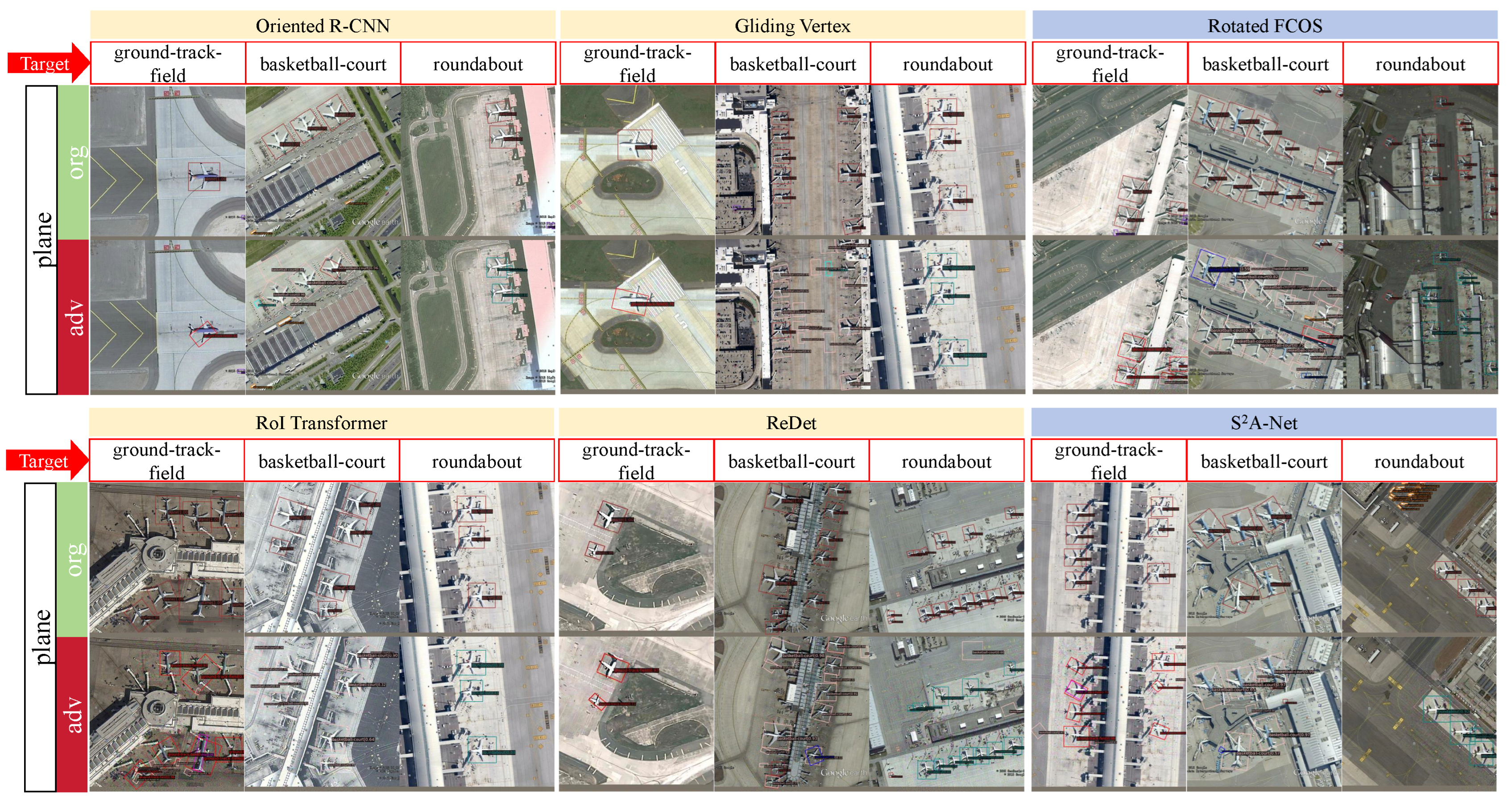
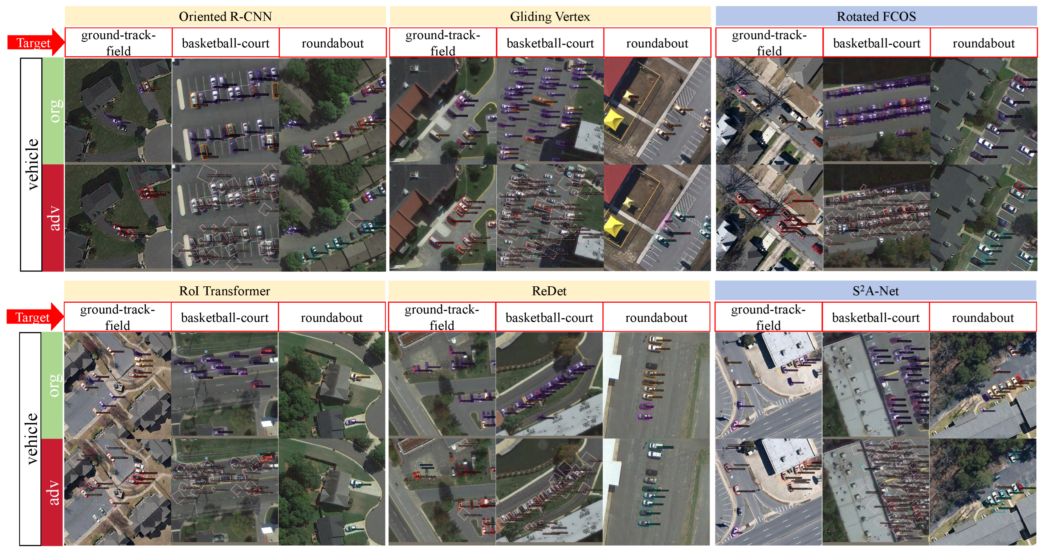
The visualization results of targeted attacks are displayed in Figure 5 and Figure 6. We can see that FFA has better attack results on different targets in different detectors.

4.4. Effect of Iteration Number

The number of iterations is a direct parameter that impacts the efficiency of the attack, so we assessed the influence of the iteration number using multiple evaluation metrics. The results are displayed in Table 5 and Figure 7.

From the results, we can see that only the attack time is positively correlated with the iteration number, and the more iteration numbers, the longer the attack time. The relationship between the attack effect and imperceptibility and the iteration number is more complicated: the attack effect is first enhanced and then weakened with the increase of iteration number, while the imperceptibility of the perturbation is exactly the opposite, first weakened and then enhanced. It shows that there is a contradiction between the attack effect and imperceptibility, and the stronger the attack effect is, the weaker the imperceptibility of the perturbation is. Since the results in the table show that the imperceptibility of the perturbation is still at a low level, taking into account, we set the iteration number of FFA to 50.

4.5. Ablation Experiment

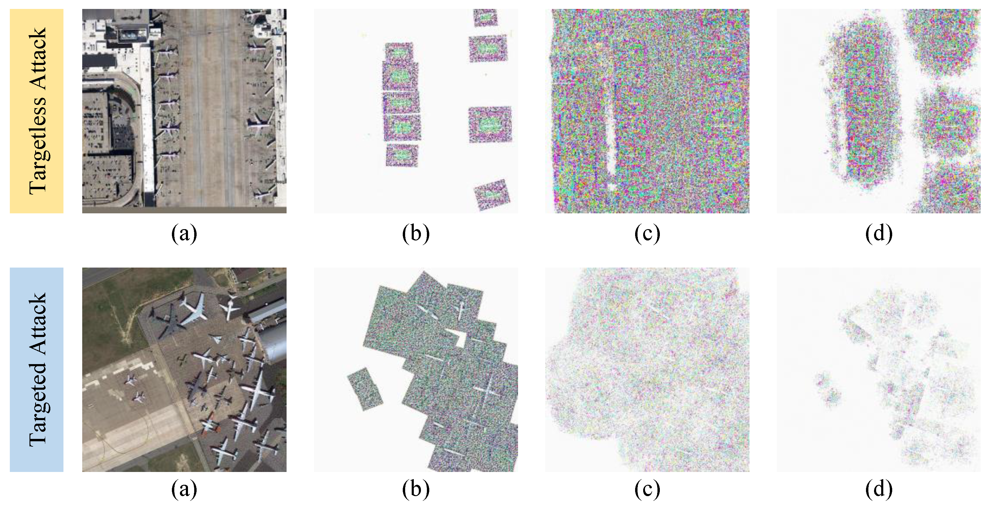
In this section, we verify the effect of different losses used in the method on the attack efficacy. The quantitative results are displayed in Table 6, and the visualization results are displayed in Figure 8.

5. Conclusion and Discussion

This work explores a strategy for generating AEs for RSOD. Most existing methods directly attack the predictive information of the image to achieve the effect of fooling the ODs. Unlike these methods, we propose an attack method that utilizes the information of the image itself by changing the feature of the image in the view of the backbone. Specifically, we first use the OD to filter out high-quality predictions as the object to implement the attack, create a hybrid foreground without any target, and use KL-divergence to minimize the shallow features of the attack object and the shallow features of the hybrid foreground to achieve a targetless attack. Replace the hybrid foreground with the target foreground and repeat the above process to realize the targeted attack. Although this method is relatively simple, the results of attacking seven rotating ODs on two datasets show that this method can generate AEs with high transferability.

There are still some directions that can be improved in this study: (1) When selecting the object to implement the attack, we use the prediction scores and IoU for threshold screening, which can result in poor-quality attack objects, leading to the weakening of the effect of the attack, and it can be improved by adding a better screening strategy. (2) The imperceptibility of the perturbation is weak. More effective perturbation control methods can be set to increase the imperceptibility of the perturbation. (3) The attack speed of the algorithm is slow, and there are still some redundant calculations in the algorithm, which increases the amount of calculation, and a more efficient iteration method can be designed to reduce the amount of calculation.

Author Contributions

Conceptualization, S.M.; methodology, L.H.; software, R.Z.; validation, R.Z., S.M. and L.H.; formal analysis, W.G.; investigation, R.Z.; resources, W.G.; data curation, R.Z.; writing—original draft preparation, R.Z.; writing—review and editing, W.G.; visualization, R.Z.; supervision, S.M. All authors have read and agreed to the published version of the manuscript.

Funding

This research received no external funding.

Institutional Review Board Statement

Not applicable.

Informed Consent Statement

Not applicable.

Data Availability Statement

The data used to support the findings of this study are available from the corresponding author upon request.

Conflicts of Interest

The authors declare no conflicts of interest.

References

Dou, P.; Huang, C.; Han, W.; Hou, J.; Zhang, Y.; Gu, J. Remote sensing image classification using an ensemble framework without multiple classifiers. ISPRS Journal of Photogrammetry and Remote Sensing 2024, 208, 190–209. [Google Scholar] [CrossRef]
Zhu, R.; Ma, S.; Lian, J.; He, L.; Mei, S. Generating Adversarial Examples Against Remote Sensing Scene Classification via Feature Approximation. IEEE Journal of Selected Topics in Applied Earth Observations and Remote Sensing 2024, 17, 10174–10187. [Google Scholar] [CrossRef]
Xu, Y.; Ghamisi, P. Universal adversarial examples in remote sensing: Methodology and benchmark. IEEE Transactions on Geoscience and Remote Sensing 2022, 60, 1–15. [Google Scholar] [CrossRef]
Gu, H.; Gu, G.; Liu, Y.; Lin, H.; Xu, Y. Multi-Branch Attention Fusion Network for Cloud and Cloud Shadow Segmentation. Remote Sensing 2024, 16, 2308. [Google Scholar] [CrossRef]
Xiao, T.; Liu, Y.; Huang, Y.; Li, M.; Yang, G. Enhancing multiscale representations with transformer for remote sensing image semantic segmentation. IEEE Transactions on Geoscience and Remote Sensing 2023, 61, 1–16. [Google Scholar] [CrossRef]
Yi, H.; Liu, B.; Zhao, B.; Liu, E. Small Object Detection Algorithm Based on Improved YOLOv8 for Remote Sensing. IEEE Journal of Selected Topics in Applied Earth Observations and Remote Sensing 2024, 17, 1734–1747. [Google Scholar] [CrossRef]
Wang, W.; Cai, Y.; Luo, Z.; Liu, W.; Wang, T.; Li, Z. SA3Det: Detecting Rotated Objects via Pixel-Level Attention and Adaptive Labels Assignment. Remote Sensing 2024, 16, 2496. [Google Scholar] [CrossRef]
He, K.; Zhang, X.; Ren, S.; Sun, J. Deep residual learning for image recognition. In Proceedings of the Proceedings of the IEEE conference on computer vision and pattern recognition; 2016; pp. 770–778. [Google Scholar]
Chen, Y.; Tang, Y.; Xiao, Y.; Yuan, Q.; Zhang, Y.; Liu, F.; He, J.; Zhang, L. Satellite video single object tracking: A systematic review and an oriented object tracking benchmark. ISPRS Journal of Photogrammetry and Remote Sensing 2024, 210, 212–240. [Google Scholar] [CrossRef]
Zhang, Y.; Pu, C.; Qi, Y.; Yang, J.; Wu, X.; Niu, M.; Wei, M. CDTracker: Coarse-to-Fine Feature Matching and Point Densification for 3D Single-Object Tracking. Remote Sensing 2024, 16, 2322. [Google Scholar] [CrossRef]
Mei, S.; Lian, J.; Wang, X.; Su, Y.; Ma, M.; Chau, L.P. A comprehensive study on the robustness of image classification and object detection in remote sensing: Surveying and benchmarking. arXiv 2023, arXiv:2306.12111. [Google Scholar] [CrossRef]
Baniecki, H.; Biecek, P. Adversarial attacks and defenses in explainable artificial intelligence: A survey. Information Fusion 2024, 102303. [Google Scholar] [CrossRef]
Szegedy, C.; Zaremba, W.; Sutskever, I.; Bruna, J.; Erhan, D.; Goodfellow, I.; Fergus, R. Intriguing properties of neural networks. arXiv 2013, arXiv:1312.6199. [Google Scholar]
Zou, Z.; Chen, K.; Shi, Z.; Guo, Y.; Ye, J. Object detection in 20 years: A survey. Proceedings of the IEEE 2023, 111, 257–276. [Google Scholar] [CrossRef]
Cui, C.; Ma, Y.; Cao, X.; Ye, W.; Zhou, Y.; Liang, K.; Chen, J.; Lu, J.; Yang, Z.; Liao, K.D.; et al. A survey on multimodal large language models for autonomous driving. In Proceedings of the Proceedings of the IEEE/CVF Winter Conference on Applications of Computer Vision; 2024; pp. 958–979. [Google Scholar]
Zhao, J.; Zhao, W.; Deng, B.; Wang, Z.; Zhang, F.; Zheng, W.; Cao, W.; Nan, J.; Lian, Y.; Burke, A.F. Autonomous driving system: A comprehensive survey. Expert Systems with Applications 2023, 242, 122836. [Google Scholar] [CrossRef]
Cai, X.; Tang, X.; Pan, S.; Wang, Y.; Yan, H.; Ren, Y.; Chen, N.; Hou, Y. Intelligent recognition of defects in high-speed railway slab track with limited dataset. Computer-Aided Civil and Infrastructure Engineering 2024, 39, 911–928. [Google Scholar] [CrossRef]
Niu, H.; Yin, F.; Kim, E.S.; Wang, W.; Yoon, D.Y.; Wang, C.; Liang, J.; Li, Y.; Kim, N.Y. Advances in flexible sensors for intelligent perception system enhanced by artificial intelligence. InfoMat 2023, 5, e12412. [Google Scholar] [CrossRef]
Li, G.; Xu, Y.; Ding, J.; Xia, G.S. Towards generic and controllable attacks against object detection. IEEE Transactions on Geoscience and Remote Sensing 2024, 1–12. [Google Scholar] [CrossRef]
Lu, J.; Sibai, H.; Fabry, E. Adversarial examples that fool detectors. arXiv 2017, arXiv:1712.02494. [Google Scholar]
Xie, C.; Wang, J.; Zhang, Z.; Zhou, Y.; Xie, L.; Yuille, A. Adversarial examples for semantic segmentation and object detection. In Proceedings of the Proceedings of the IEEE international conference on computer vision; 2017; pp. 1369–1378. [Google Scholar]
Kurakin, A.; Goodfellow, I.J.; Bengio, S. Adversarial examples in the physical world. In Artificial intelligence safety and security; Chapman and Hall/CRC, 2018; pp. 99–112. [Google Scholar]
Thys, S.; Van Ranst, W.; Goedemé, T. Fooling automated surveillance cameras: adversarial patches to attack person detection. In Proceedings of the Proceedings of the IEEE/CVF conference on computer vision and pattern recognition workshops; 2019; pp. 49–55. [Google Scholar]
Czaja, W.; Fendley, N.; Pekala, M.; Ratto, C.; Wang, I.J. Adversarial examples in remote sensing. In Proceedings of the Proceedings of the 26th ACM SIGSPATIAL International Conference on Advances in Geographic Information Systems; 2018; pp. 408–411. [Google Scholar]
Lu, M.; Li, Q.; Chen, L.; Li, H. Scale-adaptive adversarial patch attack for remote sensing image aircraft detection. Remote Sensing 2021, 13, 4078. [Google Scholar] [CrossRef]
Du, A.; Chen, B.; Chin, T.J.; Law, Y.W.; Sasdelli, M.; Rajasegaran, R.; Campbell, D. Physical adversarial attacks on an aerial imagery object detector. In Proceedings of the Proceedings of the IEEE/CVF Winter Conference on Applications of Computer Vision; 2022; pp. 1796–1806. [Google Scholar]
Lian, J.; Wang, X.; Su, Y.; Ma, M.; Mei, S. CBA: Contextual background attack against optical aerial detection in the physical world. IEEE Transactions on Geoscience and Remote Sensing 2023, 61, 1–16. [Google Scholar] [CrossRef]
Rawat, W.; Wang, Z. Deep convolutional neural networks for image classification: A comprehensive review. Neural computation 2017, 29, 2352–2449. [Google Scholar] [CrossRef]
Agnihotri, S.; Jung, S.; Keuper, M. Cospgd: a unified white-box adversarial attack for pixel-wise prediction tasks. arXiv 2023, arXiv:2302.02213. [Google Scholar]
Liu, H.; Ge, Z.; Zhou, Z.; Shang, F.; Liu, Y.; Jiao, L. Gradient correction for white-box adversarial attacks. IEEE Transactions on Neural Networks and Learning Systems 2023, 1–12. [Google Scholar] [CrossRef]
Lin, G.; Pan, Z.; Zhou, X.; Duan, Y.; Bai, W.; Zhan, D.; Zhu, L.; Zhao, G.; Li, T. Boosting adversarial transferability with shallow-feature attack on SAR images. Remote Sensing 2023, 15, 2699. [Google Scholar] [CrossRef]
Goodfellow, I.J.; Shlens, J.; Szegedy, C. Explaining and Harnessing Adversarial Examples. In Proceedings of the International Conference on Learning Representations; 2014. [Google Scholar]
Shi, Y.; Wang, S.; Han, Y. Curls & whey: Boosting black-box adversarial attacks. In Proceedings of the Proceedings of the IEEE/CVF Conference on Computer Vision and Pattern Recognition; 2019; pp. 6519–6527. [Google Scholar]
Chen, P.Y.; Zhang, H.; Sharma, Y.; Yi, J.; Hsieh, C.J. Zoo: Zeroth order optimization based black-box attacks to deep neural networks without training substitute models. In Proceedings of the Proceedings of the 10th ACM workshop on artificial intelligence and security; 2017; pp. 15–26. [Google Scholar]
Yin, F.; Zhang, Y.; Wu, B.; Feng, Y.; Zhang, J.; Fan, Y.; Yang, Y. Generalizable black-box adversarial attack with meta learning. IEEE transactions on pattern analysis and machine intelligence 2023, 46, 1804–1818. [Google Scholar] [CrossRef]
Brendel, W.; Rauber, J.; Bethge, M. Decision-based adversarial attacks: Reliable attacks against black-box machine learning models. arXiv 2017, arXiv:1712.04248. [Google Scholar]
Reza, M.F.; Rahmati, A.; Wu, T.; Dai, H. Cgba: curvature-aware geometric black-box attack. In Proceedings of the Proceedings of the IEEE/CVF International Conference on Computer Vision; 2023; pp. 124–133. [Google Scholar]
Boutros, F.; Struc, V.; Fierrez, J.; Damer, N. Synthetic data for face recognition: Current state and future prospects. Image and Vision Computing 2023, 135, 104688. [Google Scholar] [CrossRef]
Sun, Y.; Zhang, Y.; Wang, H.; Guo, J.; Zheng, J.; Ning, H. SES-YOLOv8n: automatic driving object detection algorithm based on improved YOLOv8. Signal, Image and Video Processing 2024, 18, 3983–3992. [Google Scholar] [CrossRef]
Wenqi, Y.; Gong, C.; Meijun, W.; Yanqing, Y.; Xingxing, X.; Xiwen, Y.; Junwei, H. MAR20: A benchmark for military aircraft recognition in remote sensing images. National Remote Sensing Bulletin 2024, 27, 2688–2696. [Google Scholar]
Yang, J.; Xu, J.; Lv, Y.; Zhou, C.; Zhu, Y.; Cheng, W. Deep learning-based automated terrain classification using high-resolution DEM data. International Journal of Applied Earth Observation and Geoinformation 2023, 118, 103249. [Google Scholar] [CrossRef]
Girshick, R. Fast r-cnn. In Proceedings of the Proceedings of the IEEE international conference on computer vision; 2015; pp. 1440–1448. [Google Scholar]
Wu, S.; Tan, Y.a.; Wang, Y.; Ma, R.; Ma, W.; Li, Y. Towards transferable adversarial attacks with centralized perturbation. In Proceedings of the Proceedings of the AAAI Conference on Artificial Intelligence; 2024; Vol. 38, pp. 6109–6116. [Google Scholar]
Wang, Z.; Zhang, C. Attacking object detector by simultaneously learning perturbations and locations. Neural Processing Letters 2023, 55, 2761–2776. [Google Scholar] [CrossRef]
Liu, X.; Yang, H.; Liu, Z.; Song, L.; Li, H.; Chen, Y. Dpatch: An adversarial patch attack on object detectors. arXiv 2018, arXiv:1806.02299. [Google Scholar]
Redmon, J.; Divvala, S.; Girshick, R.; Farhadi, A. You only look once: Unified, real-time object detection. In Proceedings of the Proceedings of the IEEE conference on computer vision and pattern recognition; 2016; pp. 779–788. [Google Scholar]
Xia, G.S.; Bai, X.; Ding, J.; Zhu, Z.; Belongie, S.; Luo, J.; Datcu, M.; Pelillo, M.; Zhang, L. DOTA: A large-scale dataset for object detection in aerial images. In Proceedings of the Proceedings of the IEEE conference on computer vision and pattern recognition; 2018; pp. 3974–3983. [Google Scholar]
Zhu, H.; Chen, X.; Dai, W.; Fu, K.; Ye, Q.; Jiao, J. Orientation robust object detection in aerial images using deep convolutional neural network. In Proceedings of the 2015 IEEE international conference on image processing (ICIP). IEEE; 2015; pp. 3735–3739. [Google Scholar]
Xie, X.; Cheng, G.; Wang, J.; Yao, X.; Han, J. Oriented R-CNN for object detection. In Proceedings of the Proceedings of the IEEE/CVF international conference on computer vision; 2021; pp. 3520–3529. [Google Scholar]
Xu, Y.; Fu, M.; Wang, Q.; Wang, Y.; Chen, K.; Xia, G.S.; Bai, X. Gliding vertex on the horizontal bounding box for multi-oriented object detection. IEEE transactions on pattern analysis and machine intelligence 2020, 43, 1452–1459. [Google Scholar] [CrossRef]
Ding, J.; Xue, N.; Long, Y.; Xia, G.S.; Lu, Q. Learning RoI transformer for oriented object detection in aerial images. In Proceedings of the Proceedings of the IEEE/CVF conference on computer vision and pattern recognition; 2019; pp. 2849–2858. [Google Scholar]
Han, J.; Ding, J.; Xue, N.; Xia, G.S. Redet: A rotation-equivariant detector for aerial object detection. In Proceedings of the Proceedings of the IEEE/CVF conference on computer vision and pattern recognition; 2021; pp. 2786–2795. [Google Scholar]
Lin, T.Y.; Goyal, P.; Girshick, R.; He, K.; Dollár, P. Focal loss for dense object detection. In Proceedings of the Proceedings of the IEEE international conference on computer vision; 2017. [Google Scholar]
Tian, Z.; Shen, C.; Chen, H.; He, T. FCOS: Fully convolutional one-stage object detection. arXiv 2019. arXiv 2019, arXiv:1904.01355. [Google Scholar]
Han, J.; Ding, J.; Li, J.; Xia, G.S. Align deep features for oriented object detection. IEEE transactions on geoscience and remote sensing 2021, 60, 1–11. [Google Scholar] [CrossRef]
Zhou, Y.; Yang, X.; Zhang, G.; Wang, J.; Liu, Y.; Hou, L.; Jiang, X.; Liu, X.; Yan, J.; Lyu, C.; et al. Mmrotate: A rotated object detection benchmark using pytorch. In Proceedings of the Proceedings of the 30th ACM International Conference on Multimedia; 2022; pp. 7331–7334. [Google Scholar]
Wang, Z.; Li, Q. Information content weighting for perceptual image quality assessment. IEEE Transactions on image processing 2010, 20, 1185–1198. [Google Scholar] [CrossRef]
Chow, K.H.; Liu, L.; Loper, M.; Bae, J.; Gursoy, M.E.; Truex, S.; Wei, W.; Wu, Y. Adversarial objectness gradient attacks in real-time object detection systems. In Proceedings of the 2020 Second IEEE International Conference on Trust, Privacy and Security in Intelligent Systems and Applications (TPS-ISA). IEEE; 2020; pp. 263–272. [Google Scholar]
Chen, P.C.; Kung, B.H.; Chen, J.C. Class-aware robust adversarial training for object detection. In Proceedings of the Proceedings of the IEEE/CVF Conference on Computer Vision and Pattern Recognition; 2021; pp. 10420–10429. [Google Scholar]

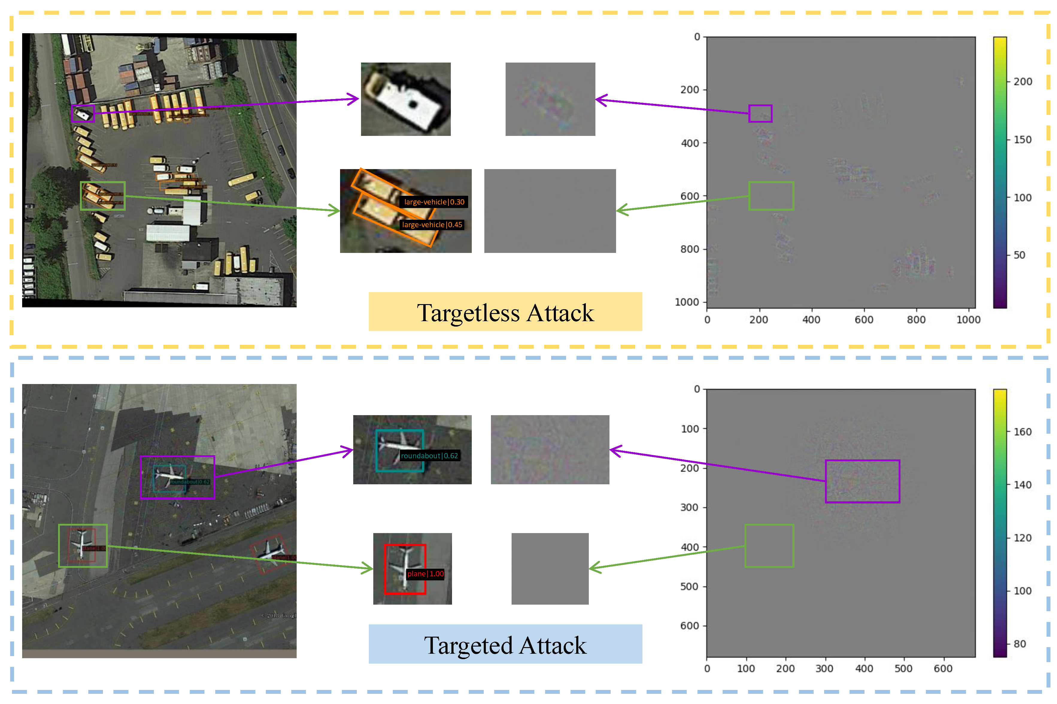
Figure 1. Illustration of the FFA realizing the targetless attack and the targeted attack. The purple box indicates the part that joins the perturbation and succeeds in the attack, and the green box indicates the part that does not join the perturbation and is recognized correctly. The orange dashed box part indicates the targetless attack, and the blue dashed box part indicates the targeted attack.

Figure 2. Visualization of the feature extraction process. The left column shows the input image, the middle column shows the foreground portion of various images, and the right column represents the corresponding shallow features of the foreground image. Blue arrows indicate the foreground extraction process, and purple arrows indicate the feature extraction process. The orange dashed box portion indicates an targetless attack, and the blue dashed box portion indicates a targeted attack.

Figure 3. Flowchart of FFA for generating AEs. Input image

x

after the detector to get the predicted foreground box

B_{p r e}

and predicted labels

l_{p r e}

. Use

B_{p r e}

to intercept the input image

x

and hybrid image

\tilde{x}

to get the input foreground

x_{f}

and hybrid foreground

\tilde{x_{f}}

. After extracting the features through the backbone, the KL-divergence of the two is calculated as the feature loss. The Smooth L1 loss between

B_{p r e}

and the real object box

B_{t r u t h}

is also calculated as the object box loss, and the cross-entropy loss between

l_{p r e}

and the background label

l_{b g}

is calculated as the classification loss, which together constitute the detector prediction loss. The sum of the L2 distance between the i-1st generated AE

x_{a d v}^{i - 1}

and

x

is calculated as the perception loss. The weighted combination of feature loss, prediction loss and perception loss yields the total loss, which is iterated to generate the adversarial perturbation

δ_{i}

, which is summed with

x

to obtain the adversarial example

x_{a d v}^{i}

after iteration.

Figure 3. Flowchart of FFA for generating AEs. Input image

x

after the detector to get the predicted foreground box

B_{p r e}

and predicted labels

l_{p r e}

. Use

B_{p r e}

to intercept the input image

x

and hybrid image

\tilde{x}

to get the input foreground

x_{f}

and hybrid foreground

\tilde{x_{f}}

. After extracting the features through the backbone, the KL-divergence of the two is calculated as the feature loss. The Smooth L1 loss between

B_{p r e}

and the real object box

B_{t r u t h}

is also calculated as the object box loss, and the cross-entropy loss between

l_{p r e}

and the background label

l_{b g}

is calculated as the classification loss, which together constitute the detector prediction loss. The sum of the L2 distance between the i-1st generated AE

x_{a d v}^{i - 1}

and

x

is calculated as the perception loss. The weighted combination of feature loss, prediction loss and perception loss yields the total loss, which is iterated to generate the adversarial perturbation

δ_{i}

, which is summed with

x

to obtain the adversarial example

x_{a d v}^{i}

after iteration.

Figure 4. Visualization of FFA targetless attack detection results. There are four layers in total. The top two layers represent the original images and AEs detection results for small objects, and the bottom two layers represent the original images and AEs detection results for large objects. The orange dashed section represents the detection outcomes of the two-stage ODs, while the blue dashed section represents the detection outcomes of the single-stage ODs.

Figure 5. Visualization of object detection results for targeted attacks against planes. The part indicated by the red arrow is the target category, the orange color is the detection result of the two-stage OD, and the blue color is the detection result of the single-stage OD.

Figure 6. Visualization of object detection results for targeted attacks against vehicles.

Figure 7. The impact of the iteration number on the attack. The trained and attacked ODs for both targetless attack and targeted attack are OR, and the backbone network is ReSNet50.

Figure 8. Visualization results of perturbations in ablation experiments. The upper layer is the targetless attack, and the lower layer is the targeted attack. (a) is the original image, (b) is the perturbation with feature loss only, (c) is the perturbation with prediction loss and feature loss, and (d) is the perturbation with feature loss, prediction loss, and perception loss.

Table 1. Targetless attack effectiveness of different adversarial attack methods on DOTA dataset.

Trained ODs/ Backbone	Attack Method	${mAP}_{50}$ ↓							IW-SSIM↓	Time↓(s/image)
		Attacked ODs
		OR	GV	RT	RD	S2A	RR	RF
	Clean	84.1	80.9	87.4	83.5	81.0	78.9	77.6	-	-
	TOG[58]	11.8	26.8	30.7	40.9	26.7	28.5	26.3	0.49	4.05
OR[49]	CWA[59]	9.2	25.7	28.5	38.5	25.6	26.3	25.5	1.31	4.23
R50	LGP[19]	4.1	19.3	21.6	35.3	22.0	20.4	20.7	0.22	6.12
	FFA(ours)	3.3	14.2	19.0	30.2	20.5	19.1	19.8	0.85	6.68
	TOG[58]	40.5	29.4	28.1	60.7	34.7	36.7	37.1	0.74	6.73
GV[50]	CWA[59]	38.1	27.6	35.9	59.4	35.4	34.2	35.3	0.86	5.81
R50	LGP[19]	32.7	23.1	33.7	56.3	32.0	30.6	32.2	0.38	7.85
	FFA(ours)	27.2	21.6	30.5	52.8	29.5	25.7	30.6	0.61	9.03
	TOG[58]	40.8	36.3	30.4	62.7	37.1	35.4	37.2	0.66	7.71
RT [51]	CWA[59]	39.3	35.1	28.6	63.1	35.8	33.6	36.4	1.07	8.34
R50	LGP[19]	35.4	29.8	20.8	60.2	32.3	30.1	32.4	0.52	10.37
	FFA(ours)	31.9	26.2	18.0	55.0	28.6	27.5	29.6	0.62	8.47
	TOG[58]	58.3	61.2	68.4	27.9	62.8	64.7	60.3	0.51	6.74
RD [52]	CWA[59]	55.7	60.1	65.5	25.1	60.6	65.4	59.5	0.87	8.80
R50	LGP[19]	53.6	55.8	60.3	22.0	58.2	61.1	57.9	0.18	9.65
	FFA(ours)	50.2	50.6	53.0	19.6	53.4	59.7	56.2	0.36	10.35
	TOG[58]	47.5	49.8	54.1	62.7	20.6	53.1	57.4	0.98	14.26
S2A [55]	CWA[59]	45.1	45.6	52.4	60.3	11.9	50.4	55.3	1.25	19.54
R50	LGP [19]	42.8	43.3	49.6	57.0	5.2	47.4	51.7	0.64	25.32
	FFA(ours)	39.3	38.9	47.8	55.4	4.5	43.6	48.2	0.74	26.47
	TOG[58]	55.7	56.4	52.1	52.8	60.3	17.3	50.1	0.83	13.67
RR[53]	CWA[59]	56.9	55.3	50.7	50.9	58.4	14.6	48.6	1.07	15.82
R50	LGP[19]	52.6	50.8	47.2	48.0	54.6	10.2	46.4	0.67	27.62
	FFA(ours)	49.3	47.1	45.8	44.9	51.0	8.5	41.5	0.75	28.46
	TOG[58]	46.5	47.9	47.4	50.5	50.4	55.7	18.3	0.71	15.65
RF[54]	CWA[59]	45.8	45.3	45.6	47.3	47.6	53.4	15.7	0.93	19.54
R50	LGP[19]	40.6	43.7	42.1	44.7	42.1	49.8	10.3	0.55	28.31
	FFA(ours)	35.1	40.5	38.6	41.7	38.2	46.3	9.2	0.69	30.66

* The most optimal outcomes in the table are emphasized in bold. Green font indicates white-box attacks. For ease of observation, the values of

{mAP}_{50}

and IW-SSIM in the table are the results after expanding the original values by a factor of 100.

Table 2. White-box targeted attack effectiveness of different adversarial attack methods on UCAS-AOD dataset.

			${mAP}_{50}$ ↓							$N_{t 0.75}$ ↑
Origin	Target	Attack Method	OR	GV	RT	RD	S2A	RF	RR	OR	GV	RT	RD	S2A	RF	RR
Plane	Clean		90.1	90.5	89.7	91	89.3	90.2	89.1	3505	3241	3359	3418	3525	3684	3457
	Ground track field	TOG[58]	25.7	22.3	21.2	25.5	17.1	15.7	10.3	2215	2339	2237	2189	2681	2706	2892
		CWA[59]	23.4	19.6	20.1	25.2	15.3	14.2	9.8	2367	2551	2342	2135	2764	2833	3085
		LGP[19]	20.2	16.7	16.1	23.1	11.9	10.2	3.7	2553	2780	2718	2554	2937	2823	3142
		FFA(ours)	18.7	13.1	12.5	19.0	7.8	6.3	1.2	2876	3108	3005	2735	3121	3027	3331
	Basket- ball court	TOG[58]	24.7	19.4	22.3	25.7	16.7	17.3	8.4	2147	2371	2287	2108	2576	2478	3059
		CWA[59]	21.3	17.3	20.5	24.4	15.2	15.2	8.9	2213	2564	2349	2235	2635	2593	2974
		LGP[19]	19.2	14.6	17.8	21.2	10.4	10.7	4.1	2632	2744	2605	2573	2854	2849	3213
		FFA(ours)	17.5	12.1	15.6	17.3	6.9	7.3	2.2	2719	2893	2819	2746	3122	3085	3397
	Round- about	TOG[58]	20.6	20.1	22.3	25.3	12.4	13.5	8.5	2368	2271	2263	2182	2403	2513	2889
		CWA[59]	19.4	18.7	20.5	22.7	10.9	11.6	5.2	2507	2584	2416	2237	2648	2678	3011
		LGP[19]	17.3	16.1	17.1	20.6	9.6	9.2	2.6	2640	2747	2661	2519	2931	2832	3234
		FFA(ours)	15.8	12.7	17.8	18.1	7.7	6.1	0.9	2841	2908	2773	2795	3086	3225	3411
Vehicle	Clean		81.5	82.3	79.8	85.2	83.1	81.6	82.7	3565	3483	3217	3238	3804	3561	3615
	Ground track field	TOG[58]	27.1	30.3	24.6	25.8	14.2	9.6	15.2	2306	2241	2048	2246	2763	3047	2971
		CWA[59]	25.3	26.7	22.3	22.6	12.4	8.3	12.5	2253	2437	2369	2517	2845	3112	3102
		LGP[19]	22.7	21.6	19.1	20.3	9.2	4.9	6.7	2537	2614	2715	2658	3183	3474	3368
		FFA(ours)	20.2	18.3	16.5	19.7	8.6	3.7	5.1	2618	2736	2823	2709	3341	3507	3472
	Basket- ball court	TOG[58]	25.5	27.6	27.0	28.9	12.4	9.8	10.7	2201	2356	2207	2087	2655	2736	2867
		CWA[59]	22.4	25.4	25.8	26.3	10.7	10.5	9.8	2351	2409	2365	2139	2813	2912	2983
		LGP[19]	19.8	20.5	19.3	22.5	8.4	7.6	5.8	2689	2654	2677	2483	3017	3202	3391
		FFA(ours)	19.6	18.7	17.9	20.7	8.0	7.6	4.4	2605	2736	2782	2625	3224	3285	3457
	Round- about	TOG[58]	28.9	29.1	22.2	26.7	16.4	12.6	11.3	2168	2145	2516	2253	2806	3013	2975
		CWA[59]	25.7	27.7	20.3	25.4	15.7	10.4	9.2	2253	2208	2453	2310	2849	3121	3010
		LGP[19]	22.4	22.3	17.8	21.6	9.6	5.8	7.1	2537	2580	2769	2544	3142	3348	3249
		FFA(ours)	21.3	19.6	16.1	21.3	10.1	5.1	6.5	2591	2674	2848	2569	3077	3403	3386

*The most optimal outcomes in the table are emphasized in bold. The green font refers to the detection result of the clean image.

Table 3. Mobility testing of targeted adversarial attack methods.

Origin	Target	Attack Method	Trained OD	${mAP}_{50}$ ↓					$N_{t 0.75}$ ↑
				Attacked ODs
				GV	RT	RD	RF	RR	GV	RT	RD	RF	RR
Plane	Basketball court	TOG[58]	OR[49]	58.6	54.5	53.5	49.1	48.5	953	1024	986	1055	1284
		CWA[59]		55.1	52.7	47.9	45.4	42.3	899	980	1443	1274	1596
		LGP[19]		48.7	46.8	44.6	39.6	35.9	1258	1386	1549	1595	1876
		FFA(ours)		45.8	43.2	42.6	37.1	34.3	1431	1503	1661	1752	1919
		TOG[58]	S2A[55]	73.8	70.6	61.5	62.2	50.5	536	683	974	961	1017
		CWA[59]		69.1	63.2	58.7	60.1	49.8	848	871	1037	1083	1385
		LGP[19]		58.5	62.7	58.3	54.4	46.1	1032	896	1096	1264	1568
		FFA(ours)		59.1	60.1	57.6	53.8	44.7	1075	935	1209	1348	1792
Vehicle	Ground track field	TOG[58]	OR[49]	70.2	69.8	69.5	65.5	68.1	753	726	774	873	754
		CWA[59]		68.5	70.4	68.7	65.2	66.3	796	698	886	912	817
		LGP[19]		65.7	67.5	65.8	63.1	64.0	905	903	1027	1108	1283
		FFA(ours)		65.1	66.3	64.4	60.9	61.7	937	971	1136	1395	1407
		TOG[58]	S2A[55]	73.2	70.7	72.3	67.3	65.1	685	751	634	890	1018
		CWA[59]		70.3	68.8	70.9	65.5	63.4	758	891	776	1068	1039
		LGP[19]		67.7	63.4	68.2	60.3	59.6	979	1008	872	1321	1237
		FFA(ours)		67.1	62.8	65.4	59.1	57.8	1021	1085	958	1377	1414

*The most optimal outcomes in the table are emphasized in bold. The two leftmost columns are the original and target categories.

Table 4. Imperceptibility and attack speed tests for targeted attacks.

Attack Method	IW-SSIM↓
Attack Method	OR	GV	RT	RD	S2A	RF	RR
TOG[58]	1.96	2.09	1.77	2.41	2.56	1.94	2.09
CWA[59]	2.53	2.74	1.98	2.37	2.91	2.04	3.62
LGP[19]	1.56	1.47	1.53	1.94	2.13	1.06	2.76
FFA(ours)	1.78	1.95	1.72	2.01	2.35	1.25	3.12
Attack Method	Time(s/image)↓
Attack Method	OR	GV	RT	RD	S2A	RF	RR
TOG[58]	4.49	5.58	6.53	7.43	6.14	7.07	5.86
CWA[59]	5.36	4.07	7.74	8.65	13.55	11.68	11.23
LGP[19]	6.83	6.15	10.62	10.31	17.54	15.47	16.21
FFA(ours)	6.95	7.81	11.83	10.47	18.75	16.29	18.58

* The most optimal outcomes in the table are emphasized in bold.

Table 5. Effect of iteration number on attack results.

Attack Method	OD/Backbone	I	1	10	20	50	100
Targetless FFA	OR/R50	${mAP}_{50}$ ↓	34.2	6.7	4.1	3.3	6.8
		IW-SSIM↓	0.21	0.20	0.32	0.85	0.12
		Time↓	0.85	2.41	4.36	6.68	13.75
Targeted FFA	OR/R50	${mAP}_{50}$ ↓	55.6	39.6	25.4	18.7	22.1
		$N_{t 0.75}$ ↑	1283	1583	2283	2876	2679
		IW-SSIM↓	0.51	0.67	1.05	1.78	1.03
		Time↓	1.03	2.29	4.71	6.95	15.33

* The most optimal outcomes in the table are emphasized in bold.

Table 6. Ablation experiments.

Targetless FFA	OR	$L_{f e a t}$	$L_{p r e}$	$L_{p e r}$	IW-SSIM↓	${mAP}_{50}$ ↓	Time↓
	Clean	-	-	-	-	83.3	-
	1	√			3.81	11.2	5.38
	2	√	√		2.51	8.9	7.45
	3	√	√	√	0.85	3.3	9.51
Targeted FFA	OR/Plane	$L_{f e a t}$	$L_{p r e}$	$L_{p e r}$	IW-SSIM↓	${mAP}_{50}$ ↓	Time↓
	Clean	-	-	-	-	90.1	-
	1	√			5.85	25.7	2.32
	2	√	√		3.64	23.9	2.96
	3	√	√	√	1.50	18.7	3.55

* The most optimal outcomes in the table are emphasized in bold. We used OR as the trained and attacked detector, and for targeted attacks, selected plane as the original category and ground track field as the target category.

Disclaimer/Publisher’s Note: The statements, opinions and data contained in all publications are solely those of the individual author(s) and contributor(s) and not of MDPI and/or the editor(s). MDPI and/or the editor(s) disclaim responsibility for any injury to people or property resulting from any ideas, methods, instructions or products referred to in the content.

© 2024 by the authors. Licensee MDPI, Basel, Switzerland. This article is an open access article distributed under the terms and conditions of the Creative Commons Attribution (CC BY) license (http://creativecommons.org/licenses/by/4.0/).

Copyright: This open access article is published under a Creative Commons CC BY 4.0 license, which permit the free download, distribution, and reuse, provided that the author and preprint are cited in any reuse.

MDPI Initiatives

Important Links

Choose an area of interest and we will send you notifications of new preprints at your preferred frequency.

Disclaimer

FFA: Foreground Feature Approximation Digitally Against Remote Sensing Object Detection

Abstract

1. Introduction

2. Related Work

2.1. Adversarial Attacks in Image Classification

2.2. Adversarial Attacks in Object Detection

2.3. Adversarial Attacks in Remote Sensing

3. Methodology

3.1. Problem Analysis

3.1.1. Location of the Perturbations

3.1.2. Magnitude of the Perturbations

3.2. Overview of the Methodology

3.3. Foreground Feature Approximation (FFA) Attack

3.3.1. Targetless Attack

3.3.2. Targeted Attack

4. Experiments

4.1. Experimental Preparation

4.1.1. Datasets

4.1.2. Detectors

4.1.3. Evaluation Metrics

4.1.4. Parameter Setting

4.2. Targetless Attack

4.3. Targeted Attack

4.3.1. White Box Attack Performance

4.3.2. Transferability Experiments

4.3.3. Imperceptibility and Attack Speed Test

4.4. Effect of Iteration Number

4.5. Ablation Experiment

5. Conclusion and Discussion

Author Contributions

Funding

Institutional Review Board Statement

Informed Consent Statement

Data Availability Statement

Conflicts of Interest

References

MDPI Initiatives

Important Links

Subscribe