
Submitted:
15 July 2024
Posted:
16 July 2024
You are already at the latest version
Abstract
In this paper I show that, opposite to what is generally assumed, when a source accretes matter at the so-called Eddington mass accretion rate M˙ed, the generated accretion luminosity Lacc is smaller than Led, the Eddington accretion luminosity that can stop accretion. I demonstrate my thesis using pieces of informations that, one by one, are well known in the accretion theory but that, for some reason, they are not considered altogether. Namely, I use the following facts: i) Lacc, in the ideal case, is equal to the rate at which kinetic energy is deposited into the accreting source; ii) radiation pressure decreases the velocity of the infalling matter; iii) the generally accepted formula Lacc=GMM˙/R is valid only if the matter is in free fall. To give a quantitative demonstration of my thesis I use two accretion models: the first is the very simple spherical accretion of zero-temperature, fully ionized hydrogen; then I use a model developed some years ago where the energy transfer between matter and radiation is taken into account. The fact that M˙ed generates a Lacc<Led can have consequences in all the cases in which one would need to model accretion with M˙>M˙ed to reproduce the observations.
Keywords:
Accretion
; Star formation
; Supermassive black holes
1. Introduction
Accretion is an important phenomenon in astrophysics and can be the only source of luminosity for those objects that do not have an internal energy production, like neutron stars or black holes. It is also important during the formation of a star because in this case too the accreting source can irradiate only the energy, or a fraction of it, due to the infalling matter that releases its kinetic energy when its fall stops.
The amount of kinetic energy that can be radiated away depends strongly on how the motion is stopped and on the efficiency of converting this energy in luminosity. In any case, energy conservations requires that if all the kinetic energy is converted in accretion luminosity, in the following, we have
being the mass accretion rate and the final velocity of the infalling matter at R, the radial position where the energy conversion happens; stands for kinetic because this definition of is based on the velocity of the particles. Note that, throughout this paper, or alone, is the accretion luminosity at R.
Equation (1) is seldom, if ever, found in papers on accretion because is, essentially always, written in this way
with M mass and R radius, in the sense described above, of the central source. When matter is in free fall, then , with final free-fall velocity, and the two above equations are equivalent: the potential energy per unit mass, , is entirely converted in kinetic energy.
The accretion luminosity exerts a force [1] that alters the motion of the matter reducing its velocity. The question arises whether the radiation pressure can ultimately halt accretion, and for which this happens. In analogy with what derived by Eddington [2] who found that the radiation pressure due to thermonuclear reactions in the interior of a star can make the stellar atmosphere evaporate1, the that stops accretion is named . For spherical accretion of ionized hydrogen, it is easy to derive [4]
where c is the velocity of light, m is the proton mass and is the Thomson cross section for electrons. If we assume that Equation (2) holds for any , we can define the Eddington mass accretion rate, , as
The fact that can be reached with a finite value of has important implications in astrophysics, for instance in topics like high-mass star formation [e.g., [5], accretion onto compact objects or growth of super massive black holes [e.g., [6]. In these cases, the observational results sometimes require to model the accretion with high rates, such that . Indeed, many works have been developed to overcome the limitation on , see, e.g., Donnan et al. [7] and references therein.
Now, the aim of this paper is to show that Equation (2) is not valid when radiation pressure is present. Clearly, measures the depth of the gravitational potential well but the effect of the radiation pressure is to reduce the velocity of the matter. It would make no sense, otherwise, to look for the value of that stops accretion. Thus, , or , while, as said, Equation (2) holds only if . In turn, this means that . The inequality might make the reader think that energy is not conserved; on the contrary, in the next sections I will show that assuming Equation (2) violates the energy conservation because it does not take into account that by decelerating the matter, radiation makes a work. The force acting on each particle is not only the accelerating gravitational force, but also the decelerating radiative force. The latter term is also due to gravitation so, in some sense, gravity is responsible of both forces.
The idea that gravitational force seems generated by a mass smaller than M, because of the radiation pressure, is not new: for instance, it can be found in Taam et al. [8] who introduced an effective mass, smaller than M, to take into account the radiative deceleration; however, they overlooked the consequence of this force reduction. If , and then the number of falling particles, increases more work is necessary to slow down the matter. In turn, this means that more gravitational energy, in the form of radiation, is used to decelerate the matter, and the fraction of this energy that is deposited at R is reduced. It is then clear that the radiation pressure acts as a negative feedback, it eats kinetic energy which can be seen as a reduction of gravitational potential energy. As a consequence, a complete accretion stop can happen, if ever, only for .
This paper is so organized: In Section 2 the two models I used are presented and discussed. In Section 3 the results of the second model, more realistic than the first one, in terms of velocity of the particles and accretion luminosity, are presented. Finally, in Section 4, the results are discussed and conclusions are given.
2. Methods
To demonstrate my thesis, I will exploit two accretion models: the first is very simple and for this reason analytical formulae can be derived, but at the price of being a bit unphysical. It is, however, often used to give a quick demonstration that when [4,9]. I will use it to show easily the consequences of adopting Equation (1) instead of Equation (2). The second model is more accurate because it takes into account the energy transfer between matter and radiation.
2.1. A Simple Spherical Accretion Model
This model is unphysical because it considers the interaction between matter and radiation but only in dynamical terms, ignoring that the radiation is absorbed by the infalling matter. As written, its utility comes from the fact that the equation of motion can be solved analytically.
A particle of mass m falling from a radius experiences two forces: i) the gravitational force down to the surface radius R that we suppose much smaller than ; and 2) the radiation pressure due to Thomson scattering. In the classical treatment of radiation [1], the radiation momentum is completely absorbed by matter at a rate where W is the energy density of the electromagnetic field and is the Thomson cross section. Since depends on the inverse of the square of the particle mass, this force acts mainly on the electrons. On the contrary, the gravitational force is larger for protons: as a consequence the flow should be treated as a two fluids plasma but assuming that we have only fully ionized hydrogen, we can treat the problem as one single fluid. In fact, the electric field arising from the interactions between protons and electrons keeps the two components coupled [10]. The force acting on each particle is then where is the intensity field and c is the light speed.
Depending on how we define the accretion luminosity, the equation of motion can be written in two different ways:
where m is the proton mass and, when ignoring absorption, we can set .
Equation (4) follows immediately from Equation (5) if the condition is imposed. However, it should be noted that means that the velocity is constant, not necessarily that everywhere, so that we have to verify that is indeed an allowed solution.
The problem is that if , clearly as well: the condition , through Equation (2), implies and, at same time, implies that . Thus, the combination of Equation (5) and Equation (2) does not admit the solution . The inconsistency comes from what has been already said: Equation (2) is valid only for matter in free fall and this is not the case. The only conclusion we can draw from setting in Equation (5) is that .
If we adopt Equation (1) and solve Equation (6), it is immediate to derive
from which
with . Thus
where is the final velocity for matter in free-fall: as expected, when . The solution is acceptable asymptotically, it is approached as .
By combining Equation (1) with Equation (9), after some algebra one derives
showing that , like , is asymptotically reached for .
In this way we can see that increasing increases as well. But taking into account the negative feedback of the radiation pressure, that is feeded by the gravitational potential well, the increase in luminosity does not scale linearly with .
2.1.1. The Case
In Equation (6), the luminosity produced internally by the accreting source, named in the following , has been assumed to be zero. In case , the equations change but the final result is, qualitatively, not different from the previous case, provided that .
Equation (6) becomes
with ; Equation (8) is now
and
so that
Thus, accretion is still possible with any provided that . When , the radiation pressure due to that clearly does not depend on , stops accretion.
The accretion luminosity is easily derived:
with for .
2.2. A More Realistic Accretion Model
In the previous section we have seen the consequences of defining the accretion luminosity following Equation (1) or Equation (2), by using a simple model. This model is based on three assumptions: i) zero-temperature flow, so that no interaction between particles is taken into account; ii) no energy exchange between matter and radiation; iii) decreases with radius only by the geometrical factor , which implies a constant otpical depth at all radii.
Now, assumption i) makes the model not too much realistic even if not unphysical. But assumptions ii) and iii) are not consistent with the fact that the interaction between radiation and matter must happen in order to justify the equation of motion given either by Equation (5) or by Equation (6).
Now, assumption i) makes the model not too much realistic even if not unphysical. But assumptions ii) and iii) are not consistent with the fact that the interaction between radiation and matter must happen in order to justify the equation of motion given either by Equation (5) or by Equation (6).
In this section, thus, I will employ a more realistic accretion model. In literature one can find accurate accretion models that describe the physics of the accretion process, e.g., Fukue [11] or Murakami et al. [12], just to make a few of examples. Adapting these models to my needs, however, is not simple because in many cases the use of Equation (2) is not written explicitly, so that it is not immediate to find out how to modify a given model to adopt Equation (1). And, as I am going to show, it can happen that Equation (2) and Equation (1) are unintentionally adopted at the same time.
For these reasons, I use a model developed fifty years ago by Maraschi et al. [13], MTR in the following, that while considering the exchange between matter and radiation, so assumption ii) above is no longer present, it is still quite simple.
The set of equations used by MRT is:
where the multiplying 4/3 factor in front of was added by Kafka and Mészáros [14]; note also that I have assumed a negative velocity, so the sign in the continuity equation and in the term is opposite to MRT’s set.
Equation (18) gives
where the constant is found assuming that particles’ energy goes to zero as . Now, if we analyze carefully Equation (20), we will see that it implies Equation (1) even if MTR assumed explicitly that Equation (2) holds. In fact, Energy E is given by
while the accretion luminosity is ; for we have
so that, in MTR’s model there is the hidden adoption of Equation (1). Of course, if one assumes that , that is, that the final velocity is equal to the free-fall final velocity, the two formulations of give the same result. But MRT derived for their model the velocity profile , finding that for any , it is always , which is expected. Then we have
which shows that MTR’s model was not internally consistent. Of course, my aim is not to show the inconsistency of MTR’s work, I make these considerations only to explain why I adopt a simple model instead of a complex and much more realistic, accretion model. Only in this way I can go deep in the physics of the solution to read behind the lines what are all the assumptions, intentionally or not, of the model.
Now, for we have
where the equal sign holds when for . By comparing Equation (23) with Equation (24), we have to conclude either that two equations are not consistent, or that increase with r, which looks unphysical. The reason of the inconsistency comes from neglecting the absorption of the radiation, but this problem becomes evident only if Equation (1) is assumed, because with Equation (2) it is clear that .
The set of Equations (17) — (19) cannot be solved under the assumption iii) (i.e., , see the beginning of this section). We have to take into account the absorption of the radiation by writing
with
( will be used later on in this section).
By combining the different equations, it is possible to arrive to a second order differential equation in v: all the steps are detailed in Appendix A where the general case is treated. Here I present the final equation for the case :
with , and, for typical neutron stars,
so that Equation (26) becomes
with because .
When Equation (27) turns into
and it is easy to verify that the free-fall velocity is a solution.
Let’s now see if a solution , say (no force), is possible. Equation (27) becomes
A constant solution, by definition, must be valid for any z, in particular also for where the previous equation simplifies in
from which
It is convenient to plot this cubic equation to look for the solutions: this is done in Figure 1 for a set of values of . The case is not shown because it corresponds to matter in free fall and V cannot be constant; for , a curve not shown in the figure, a solution for is not found because the curve, in the range shown, never intersects the line . A value of that is solution of the cubic equation starts appearing somewhere in the range . But for , the range of values explored in the next section, Equation (27) admits only , so that is not acceptable: as a consequence, Equation (27) does not admit a solution and, in turn, this means that the total force acting on each particle can never be zero.
3. Results
Equation (27) has been solved using the solver Radau of the routine solve_ivp, part of the Python package scipy [15], using an iterative approach2: first, Equation (8), that in adimensional variables becomes
is used in Equation (29) to derive a first estimate of the optical depth, namely
With the above , Equation (27) is solved with boundary conditions
where
Once and are derived, is computed again but now directly from Equation (29). The new curve is used in Equation (27) and the procedure is iterated. Given two iterations, i and , the iterations is stopped once .
This approach works for . When , decreases until reaches a minimum, then it oscillates between two values, one small and one large. In these cases, I stop the procedure once , and the solution corresponding to iteration i is used as solution.
I have also tried another approach in which, given the new solution of , Equation (27) is solved starting from and going to larger z. The optical depth is computed at runtime through
This approach failed because sometime the routine solve_ivp calls the integrating function twice with the same3z, but the second time the first derivative of V jumps to high values and diverges.
Five values of are chosen for this work: 0.1, i.e., one tenth of , 0.5, 1.0, 1.5 and 2.0. In Table 1, for each , column Iteration gives how many iterations are necessary to reach convergence (); for the other values of , the two last iterations are reported, once starts oscillating between two values. In these case, the iterations are stopped when and the adopted is the one corresponding at the smallest : for instance, when the last decreasing value is for iteration 9, and the adopted is 4.0739.
In Figure 2, the curves are shown. Because of the lack of convergence of , it is possible that is a bit overestimated for .
The solutions are shown in the left panel of Figure 3: at large distances they are similar, approaching the asymptotic law given by Equation (34). At short radii, , when a maximum in starts appearing, clearly visible in the right panel of Figure 3 where a zoom-in of the left panel for small z is shown.
This means that infalling particles are accelerated up to very close to the surface of the accreting object, and then, at , they are strongly decelerated. In a complete thermodynamical treatment, this behaviour would be modelled with a schock, causing a strong increase in temperature. The presence of a shock was already foreseen by Shapiro and Salpeter [16], and even at similar distances; it is, however, surprising that the possibility of a shock is suggested even with a simple, zero-temperature approach as in this case. Clearly, lacking a proper thermodynamical set of equations, we can only note that the strong deceleration looks like a shock, but nothing more can be said.
Finally, in Figure 4 the luminosity is shown, where
As expected, follows the trend of modulated by the exponential of . As said before, however, it is likely that the optical depth is overestimated at large z, so that, especially for , the luminosity might be underestimated.
Figure 4 gives a quantitative representation of what has been said at the end of the Introduction: for high , the work done by the radiation pressure to decelerate the infall matter makes the emerging luminosity be more and more faint. This is because even if the number of particles increases with , the kinetic energy per particle is more and more reduced.
4. Discussion
We have seen that Equation (20) implies Equation (1), so it could seem that the aim of this paper, to promote the use of instead of the more common , is not new: even if not explicitly written, we can find that equation already in a fifty-years-old model. Moreover, Equation (2) is often not explicitly written in modern accretion models, as if it were not used.
However, Equation (2) is at the base of the following equivalence, used in pratically all the papers on accretion:
No matter how is written, the above equivalence clearly states that when then , and once accretion is stopped.
On the contrary, if one follows Equation (1), then
as a consequence, not only does not imply that the accretion luminosity is equal to , also, it is to be demonstrated that can ever be reached with a finite .
I have derived Equation (40) first using a basic accretion model that has the only advantage to give an analytical expression for the velocity law .
Once is known, can be computed and one can see that is an asymptotic value reached only for . In this model, when we have .
I have then adopted a second accretion model developed by MTR. This model is more realistic than the first one, but with a strong assumption: the falling particles do not interact each other during the motion. This is equivalent to say that the flow is at zero-temperature. Such an assumption is, of course, less than optimal and the results obtained are, with no doubt, of limited value. However, it is important to stress that this model is not unphysical, no physical law is violated, it is only not too much realistic. It can be seen as an ideal experiment of thermodynamics that cannot be executed in real world but that can give indications on how a system evolves. The model used here can give insights on what happens in the accretion flow when Equation (1) is used.
I understand that the reader can feel uncomfortable if someone claims that what has been assumed in the last sixty years, Equation (2) or Equation (39), is not correct. But my conclusion is based on Equation (1): first, it is based on energy conservation; second, it was already used in the past, as shown before. Equation (2) violates the energy conservation because it does not take into account that the radiation pressure makes work on the infalling matter, changing the equation of motion. As a consequnce, also the energy balance must be adapted. It is clear that the depth of the gravitational potential well remains , independent on . On the other hand, the radiation pressure acts as a counter-reaction whose amplitude is a fraction of , and one has to demostrate that this fraction can indeed be 1.
All the accretion models show that the matter is not in free fall, being decelerated by the radiation pressure, thus Equation (2) can no longer be valid and Equation (40) holds. For any developed accretion model, it has to be demonstrated that radiation pressure can halt accretion with a finite , this assumption must be proved and, in general, for is not reached.
Funding
This research received no external funding.
Data Availability Statement
All the python routine used in this work are freely available at https://drive.google.com/drive/folders/0ADGdDSs8TC5WUk9PVA.
Acknowledgments
Preliminary versions of this paper were read by Prof. Francesco Strafella and Dr. Patrick Hennebelle, who I kindly thank for their suggestions. I wish also to thank Ms. Anne Zhang, Managing Editor of Universe, for being patient with all the delays in the submission of the work.
Conflicts of Interest
The author declares no conflicts of interest.
Appendix A
In this section, the system of Equations (16)–(19) will be used to derive the second order differential equation in V, Equation (27), in the more general case of , the internal luminosity of the accreting source, different from zero. By setting in the following , all the equations given in Section 2.2 can be recovered.
First, Equation (25) becomes
with given by Equation (26).
Then, I follow MTR’s procedure: first, combining Equation (A1) with Equation (19) we have
and using Equation (16)
from which
To eliminate U, Equation (A4) is derived with respect to r and Equation (16) is used again. But before that, I write E as a function of v, differently from MTR who wrote v as a function of E,
so that
and
Thus
and after expanding all the multiplications
After simplifying the term we get
that can be cast in this form
Now we use the relation
so that
and finally
It might be of some interest to note that the equation for E derived by MTR contains the term , while in the above equation a quadratic term in is not present.
At this point, the following dimensionless variables are introduced: , , obtaining
with
where
is the final free-fall velocity;
and, finally,
All the terms can be collected and the common factor can be cancelled out, obtaining
Equation (27) corresponds to Equation (A28) once is set to zero. The procedure to compute the solution is the same outlined in Section 3: the initial is derived assuming the velocity law given by Equation (14) that, in the new variables, becomes
Thus, Equation (35) is now
Equation (A28) has been resolved for two values of , 0.1 and 1.0, and two values of , 0.1 and 0.5. If , V changes sign so that Equation (17) and Equation (19) must be changed as well. However, the case of reverted motion is out of the scope of this paper and will not discussed.
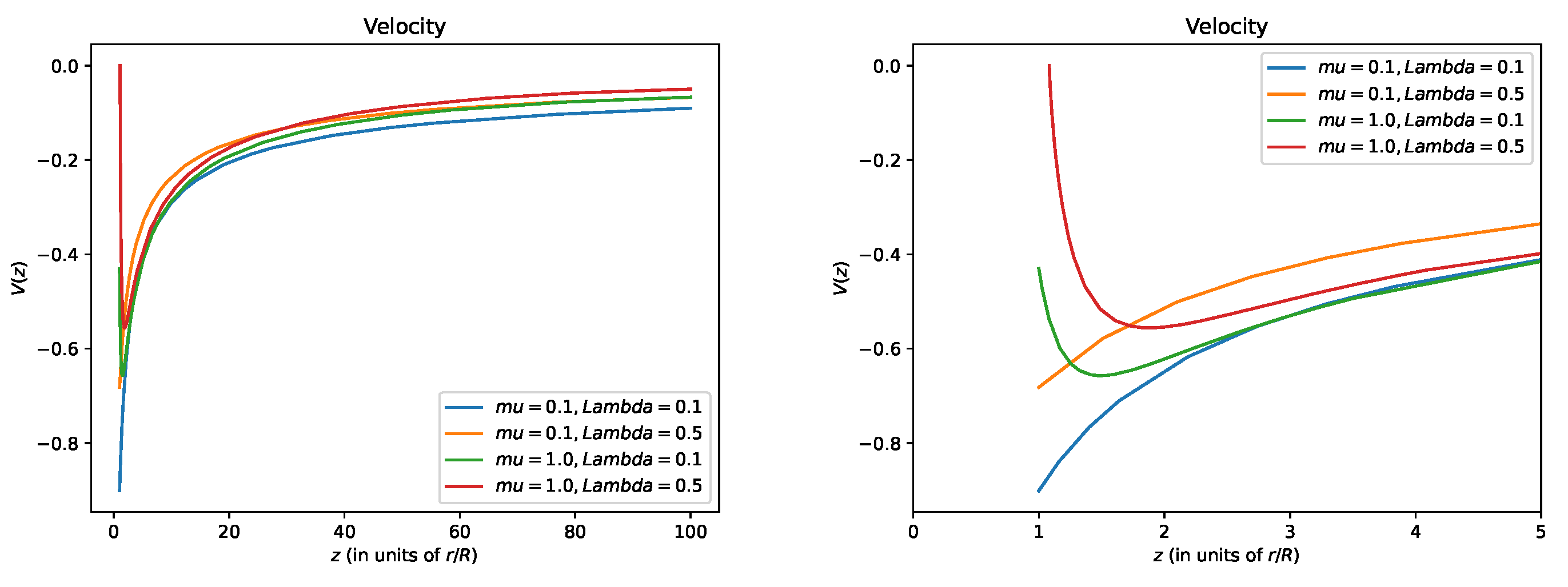
In Figure A1 the solutions of are reported for the four cases studied. The two panels are quite similar to those in Figure 3. The main difference is that does not depend on , nor on , so that, at the surface of the accreting object, the radiation pressure is higher than in the case of causing a stronger deceleration.
Figure A1.
Left panel: velocity V, in units of free-fall velocity vs. normalized radial distance for two values of , in units of , and two values of , in units of . Right panel: zoom-in of the left figure to emphasize the maximum in at short radii.
Figure A1.
Left panel: velocity V, in units of free-fall velocity vs. normalized radial distance for two values of , in units of , and two values of , in units of . Right panel: zoom-in of the left figure to emphasize the maximum in at short radii.
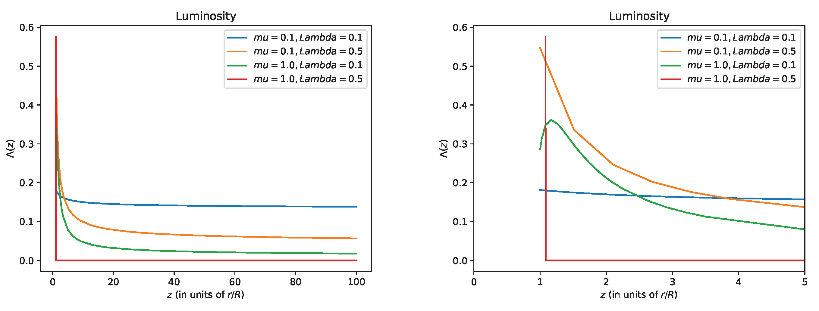
The luminosity profile, given by
is shown in the two panels of Figure A2. For and , the optical depth increases so fast that the luminosity goes to very small values just above the surface of the accreting object. However, as written in Section 2.2, the procedure used to solve Equation (A28) causes a likely overestimated of : a more rigorous treatment of accretion, without the zero-temperature assumption, would probably give a more gentle transition in V when z approaches 1, and, consequently, a less severe attenuation of at high . In any case, at least qualitatively, we can conclude that does not stop accretion.
Figure A2.
Left panel: luminosity , in units of , vs. normalized radial distance for different values of in units of . Right panel: zoom-in of the left figure at short radii.
Figure A2.
Left panel: luminosity , in units of , vs. normalized radial distance for different values of in units of . Right panel: zoom-in of the left figure at short radii.
References
- Landau, L.D.; Lifshitz, E.M. The classical theory of fields; 1971.
- Eddington, A.S. On the radiative equilibrium of the stars. Mon. Not. R. Astron. Soc. 1916, 77, 16–35. [Google Scholar] [CrossRef]
- Abramowicz, M.A. Super-Eddington black hole accretion: Polish doughnuts and slim disks. Growing Black Holes: Accretion in a Cosmological Context; Merloni, A.; Nayakshin, S.; Sunyaev, R.A., Eds., 2005, pp. 257–273, [arXiv:astro-ph/astro-ph/0411185]. [CrossRef]
- Frank, J.; King, A.R.; Raine, D.J. Accretion power in astrophysics; 1985.
- Zinnecker, H.; Yorke, H.W. Toward Understanding Massive Star Formation. Ann. Review of Astron. & Astroph. 2007, arXiv:astro-ph/0707.1279]45, 481–563. [Google Scholar] [CrossRef]
- Inayoshi, K.; Visbal, E.; Haiman, Z. The Assembly of the First Massive Black Holes. Ann. Review of Astron. & Astroph. 2020, arXiv:astro-ph.GA/1911.05791]58, 27–97. [Google Scholar] [CrossRef]
- Donnan, F.R.; Hernández Santisteban, J.V.; Horne, K.; Hu, C.; Du, P.; Li, Y.R.; Xiao, M.; Ho, L.C.; Aceituno, J.; Wang, J.M.; Guo, W.J.; Yang, S.; Jiang, B.W.; Yao, Z.H. Testing super-eddington accretion on to a supermassive black hole: reverberation mapping of PG 1119+120. Mon. Not. R. Astron. Soc. 2023, arXiv:astro-ph.GA/2302.09370]523, 545–567. [Google Scholar] [CrossRef]
- Taam, R.E.; Fu, A.; Fryxell, B.A. Accretion in Wind-driven X-Ray Sources. The Astroph. Journal 1991, 371, 696. [Google Scholar] [CrossRef]
- Eckart, A.; Schödel, R.; Straubmeier, C. The black hole at the center of the Milky Way; 2005.
- Maraschi, L.; Reina, C.; Treves, A. On Spherical Accretion near the Eddington Luminosity. Astron. & Astroph. 1974, 35, 389. [Google Scholar]
- Fukue, J. Bondi Accretion onto a Luminous Object. Pub. of the Astroph. Soc. of Japan 2001, 53, 687–692. [Google Scholar] [CrossRef]
- Murakami, M.; Nishihara, K.; Hanawa, T. Self-Similar Gravitational Collapse of Radiatively Cooling Spheres. The Astroph. Journal 2004, 607, 879–889. [Google Scholar] [CrossRef]
- Maraschi, L.; Reina, C.; Treves, A. On Spherical Accretion near the Eddington Luminosity. Astron. & Astroph. 1974, 35, 389. [Google Scholar]
- Kafka, P.; Mészáros, P. How fast can a black hole eat? General Relativity and Gravitation 1976, 7, 841–846. [Google Scholar] [CrossRef]
- Virtanen, P.; Gommers, R.; Oliphant, T.E.; Haberland, M.; Reddy, T.; Cournapeau, D.; Burovski, E.; Peterson, P.; Weckesser, W.; Bright, J.; van der Walt, S.J.; Brett, M.; Wilson, J.; Millman, K.J.; Mayorov, N.; Nelson, A.R.J.; Jones, E.; Kern, R.; Larson, E.; Carey, C.J.; Polat, İ.; Feng, Y.; Moore, E.W.; VanderPlas, J.; Laxalde, D.; Perktold, J.; Cimrman, R.; Henriksen, I.; Quintero, E.A.; Harris, C.R.; Archibald, A.M.; Ribeiro, A.H.; Pedregosa, F.; van Mulbregt, P.; SciPy 1. 0 Contributors. SciPy 1.0: Fundamental Algorithms for Scientific Computing in Python. Nature Methods 2020, 17, 261–272. [Google Scholar] [CrossRef] [PubMed]
- Shapiro, S.L.; Salpeter, E.E. Accretion onto neutron stars under adiabatic shock conditions. The Astroph. Journal 1975, 198, 671–682. [Google Scholar] [CrossRef]
| 1 | On the validity of this attribution, see Abramowicz [3]. |
| 2 | The routine code is available for download, see paragraph Data Availability Statement toward the end of the paper. |
| 3 | It can also happen that , but this case is handled easily. |
Figure 1.
The intersections of the straight (black line) with the set of curves, drawn with different , give the value that solve Equation (33). As explained in the text, an acceptable solution for our problem requires that intersects the line for negative values. For this does not happen: Equation (27) does not admit a solution .
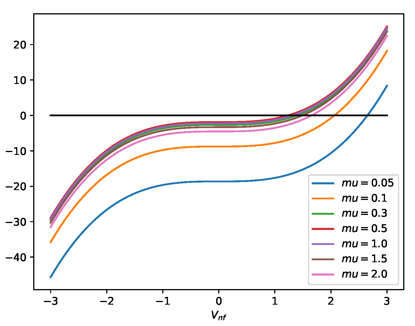
Figure 2.
Optical depth vs. normalized radial distance for different values of in units of .
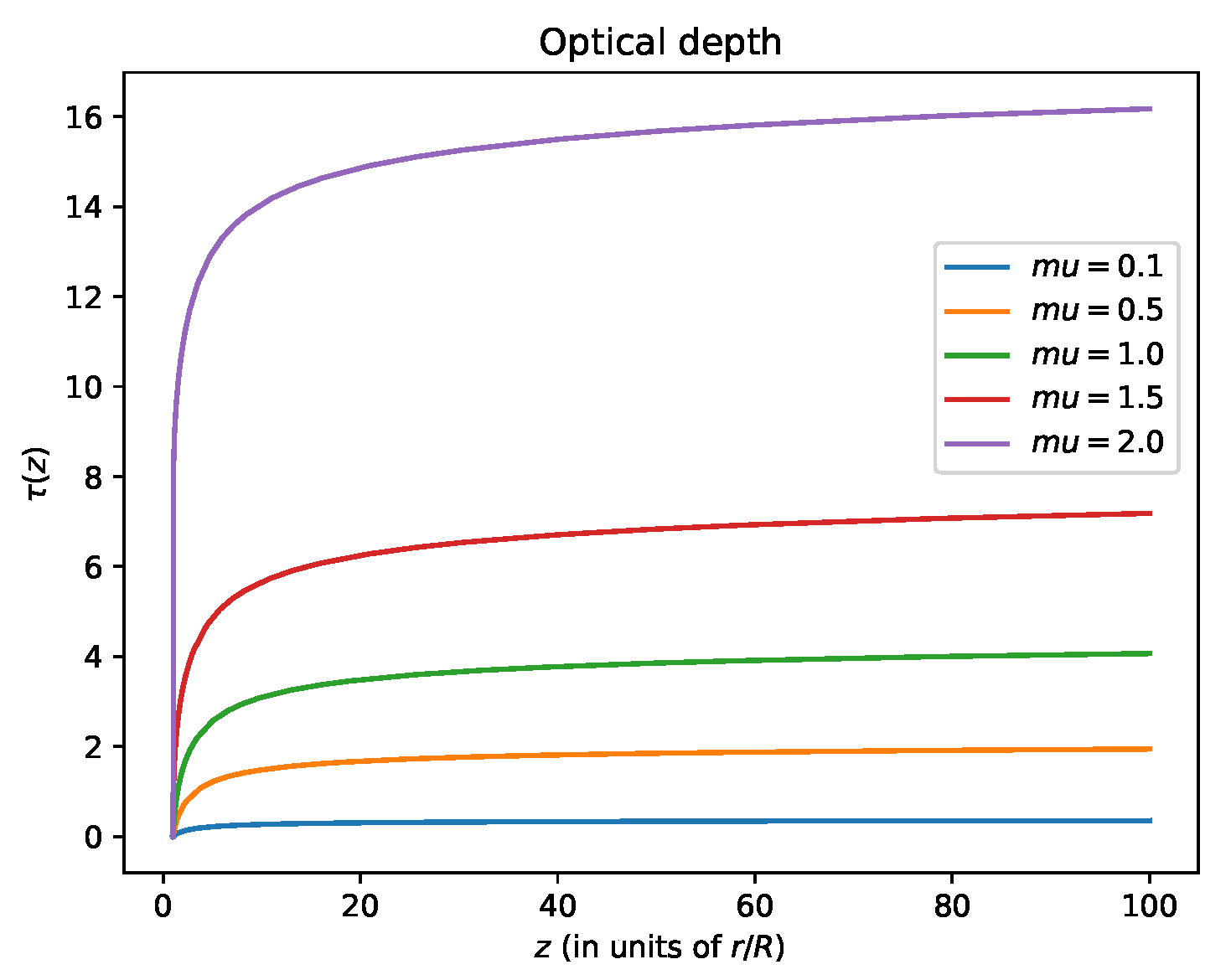
Figure 3.
Left panel: velocity V, in units of free-fall velocity vs. normalized radial distance for different values of in units of . Right panel: zoom-in of the left figure to emphasize the maximum in at short radii.
Figure 3.
Left panel: velocity V, in units of free-fall velocity vs. normalized radial distance for different values of in units of . Right panel: zoom-in of the left figure to emphasize the maximum in at short radii.
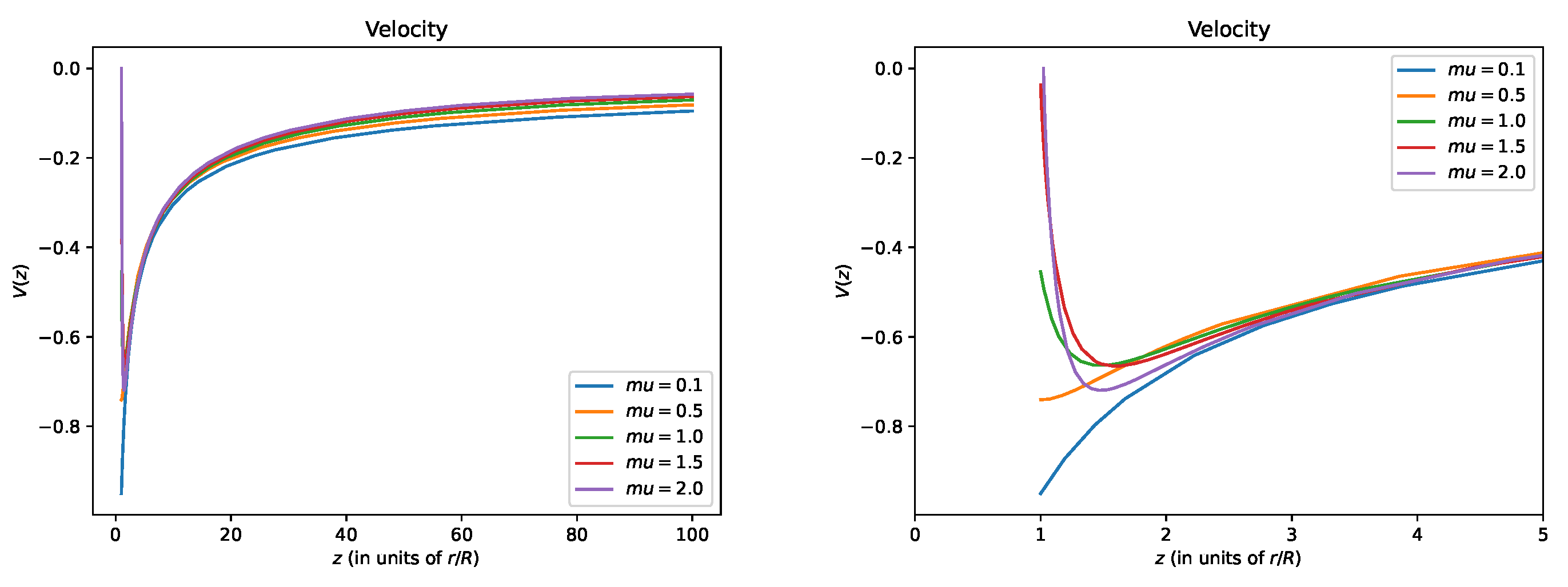
Figure 4.
Left panel: luminosity , in units of , vs. normalized radial distance for different values of in units of . Right panel: zoom-in of the left figure at short radii.
Figure 4.
Left panel: luminosity , in units of , vs. normalized radial distance for different values of in units of . Right panel: zoom-in of the left figure at short radii.
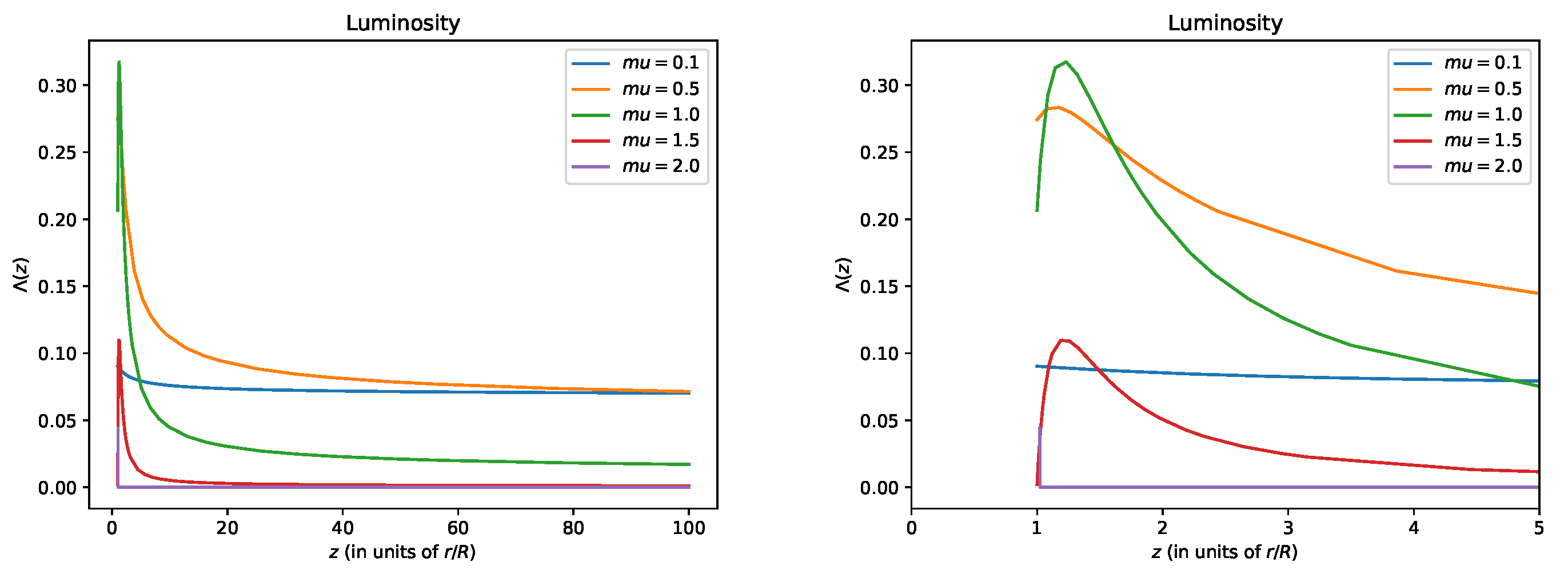

Table 1.
Here I report, for each value of , the number of iterations; and , the optical depth at the largest distance from the accreting object, where i corresponds to the number of iterations; the relative difference of the optical deptth at infinity, between two successive iterations.
Table 1.
Here I report, for each value of , the number of iterations; and , the optical depth at the largest distance from the accreting object, where i corresponds to the number of iterations; the relative difference of the optical deptth at infinity, between two successive iterations.
| Iteration | ||||
|---|---|---|---|---|
| 0.1 | 2 | 0.3518 | 0.3518 | |
| 0.5 | 4 | 1.9420 | 1.9419 | |
| 1.0 | 9 | 4.0648 | 4.0739 | |
| 10 | 4.0748 | 4.0648 | ||
| 1.5 | 2 | 7.1799 | 6.1722 | |
| 3 | 5.7619 | 7.1799 | ||
| 2.0 | 1 | 16.175 | 11.471 | |
| 2 | 7.6956 | 16.175 | 1.102 |
Disclaimer/Publisher’s Note: The statements, opinions and data contained in all publications are solely those of the individual author(s) and contributor(s) and not of MDPI and/or the editor(s). MDPI and/or the editor(s) disclaim responsibility for any injury to people or property resulting from any ideas, methods, instructions or products referred to in the content. |
© 2024 by the authors. Licensee MDPI, Basel, Switzerland. This article is an open access article distributed under the terms and conditions of the Creative Commons Attribution (CC BY) license (http://creativecommons.org/licenses/by/4.0/).
Copyright: This open access article is published under a Creative Commons CC BY 4.0 license, which permit the free download, distribution, and reuse, provided that the author and preprint are cited in any reuse.


