Preprint
Article

PyRAMD Scheme: A Protocol for Computing the Infrared Spectra of Polyatomic Molecules Using Ab Initio Molecular Dynamics

Altmetrics

Downloads

145

Views

105

Comments

0

A peer-reviewed article of this preprint also exists.

This version is not peer-reviewed

Submitted:

15 July 2024

Posted:

17 July 2024

You are already at the latest version

Alerts
Abstract
Here, we present a general framework for computing the infrared anharmonic vibrational spectra of polyatomic molecules using the Born-Oppenheimer molecular dynamics (BOMD) with the software PyRAMD. To account for the nuclear quantum effects, we suggest using the simplified Wigner sampling (SWS) approach [\textit{Phys. Chem. Chem. Phys.}, 2023, \textbf{25}, 18406-18423] simultaneously coupled with the Andersen and Berendsen thermostats. We propose a new criterion for selecting the parameter of the SWS based on the molecules' harmonic vibrational frequencies and usage of the large-time-step blue shift correction, allowing for a decrease in computational expenses. For the Fourier transform of the dipole moment autocorrelation function, we propose to use the regularized least-squares analysis, which allows us to obtain higher frequency resolution than the direct application of fast Fourier transform. Finally, we suggest the usage of the pre-parameterized scaling factors for the IR spectra from BOMD, also providing the scaling factors for the spectra at the BLYP-D3(BJ)/6-31G, PBE-D3(BJ)/6-31G, and PBEh-3c levels of theory.
Keywords: 
Subject: Chemistry and Materials Science  -   Theoretical Chemistry

1. Introduction

Molecular dynamics (MD) is the method of describing nuclear motions using classical mechanics [1,2,3,4]. If the potential energy surface (PES) for the simulation is taken from the quantum-chemical calculations, such simulations are called ab initio MD (AIMD) [4]. AIMD is a powerful tool for simulating various physical observables of medium to large systems (from tens to a few hundreds of atoms) with non-trivial dynamical behavior [3,4,5,6]. Examples of modeled observables can be radial distribution functions in diffraction experiments [7,8,9,10], dynamical properties of solutions [6,11], and various types of spectra [5,12,13]. Calculating of the spectral response in the case of electronic excitations, such as ultraviolet or X-ray spectroscopy, usually relies on sampling the conformational space of molecular systems [12,14]. In contrast, in the case of the vibrational spectra, i.e., infrared (IR) [4,5,10], Raman [13], vibrational circular dichroism [15], etc., the fluctuation-dissipation theorem (FDT) [16,17] has to be applied.
The bare AIMD simulations, by definition, model the motion of classical particles, thus producing a classical microcanonical ( N V E ) ensemble [18]. To emulate the canonical ensemble ( N V T or N P T ), an artificial external system (thermostat and/or barostat) is added to the MD simulations [18]. As the real nuclei are quantum objects, the absent nuclear quantum effects (NQEs) can also be accounted for in the MD by various approaches [19], such as path-integral MD [20,21], quantum thermostats [22], Wigner sampling [14,23,24], etc. [19]
In this work, we provide a protocol for simulating the IR spectra of molecules with BOMoND software. This MD interface software can take energies and gradients from the quantum-chemical package ORCA 5 [25] or the semi-empirical package xTB [26]. The BOMoND is part of the PyRAMD packet for AIMD-based simulations, which is also capable of metadynamics [27] and MD-based mass-spectra calculations [28]. We will demonstrate examples of applications of BOMoND software, illustrating the various aspects of the MD procedure and subsequent analysis.

2. Methods

The results presented here were obtained using the BOMoND software from the PyRAMD package [29]. This software can be obtained from the corresponding repository (Ref. [29]). The density functional theory (DFT) calculations[30] at the BLYP-D3(BJ)/6-31G,[31,32,33,34] PBE-D3(BJ)/6-31G,[33,34,35] and PBEh-3c[36] and semi-empirical calculations at the GFN2-xTB levels of theory [37], including structure optimization and harmonic frequencies computation, were done using ORCA 5 [25] and xTB software [26], respectively. The BOMoND used the same program suits to get the gradients for the AIMD simulations. The dipole moment autocorrelation functions calculations and the subsequent Fourier transform (FT) [38] and regularized least-squares spectral analysis (rLSSA) [39] were done using the script from the PyRAMD package.

3. Simulation Protocol for the Vibrational Spectra Using the Molecular Dynamics

3.1. General Idea of Calculation of the IR Spectra from MD Trajectories

The MD simulation produces an MD trajectory, N steps simulations points, which span the dynamics in time t from t = 0 to N steps · Δ t , where Δ t is the time step of the simulation. Therefore, for various computed physical observables ( O , e.g., coordinates, velocities, energy, dipole moment, polarizability, etc.), we can tell their values ( O ( n · Δ t ) = O n ) at a n-th given point of simulation ( 0 n < N steps ), corresponding to the time t = n · Δ t [18].
As said in the introduction, the vibrational spectra from MD are computed with the help of the FDT [16,17]. We first need to compute the autocorrelation function ( O ( 0 ) · O ( t ) ) of the variable O that is responsible for the response to the external excitation. For the IR spectra, observable is the total dipole moment of the molecule; for the Raman spectra, it is the molecular polarizability tensor; for the power spectrum, these are simply the mass-weighted coordinates, etc. [13]. For a real-valued observable, the autocorrelation function is defined as [4,5,13,40]
O ( 0 ) · O ( t ) = 0 O ( t ) O ( t + t ) d t ,
and it shows the repeatable periods in the time evolution of the given observable. The numerical calculation of the autocorrelation function for finite time series is available in various packages. For instance, in Python, one could use either the “correlate” method from the NumPy module [41] or the “signal.correlate” method from the SciPy module [42]. By performing the FT of the O ( 0 ) · O ( t ) as [4,5,13,40]
S ( ν ) = ν 2 0 O ( 0 ) · O ( t ) · exp ( i 2 π ν ) d t
we can transfer the response characteristic from the time domain (t) to the frequency domain ( ν ), thus obtaining the spectrum of a given process. For numerical reasons, a more advantageous computational strategy is to use the velocity of the observable ( O ˙ ) to obtain the spectrum [5]. In this case, the expression to be used is[5]
S ( ν ) = 0 O ˙ ( 0 ) · O ˙ ( t ) · exp ( i 2 π ν ) d t .
The resulting spectra from Equations 2 or 3 can be multiplied with the correction factors that account for the statistical properties at the different spectral ranges [5,43].
The FT procedure on the MD results (Equation 2 or 3) is usually done using a fast-FT (FFT) approach [38,44], which provides certain limitations on the frequency discretization of the resulting spectra. The frequency grid increment ( Δ ν ) is determined by the total trajectory duration τ tot through the Nyquist–Shannon–Kotelnikov (NSK) theorem [45,46,47] as Δ ν = 1 / τ tot , while the time step Δ t determines the upper boundary of the spectrum as ν max = 1 / Δ t . To increase the formal resolution, extending the trajectory for a given observable by an arbitrary number of steps with zeros is possible, which is called zero-padding [48]. However, such direct extension will cause artifacts in the resulting spectrum; thus, the zero-padding should be combined with either frequency filters or smoothing techniques [39,48].
An alternative procedure to the FFT could be the regularized least-squares spectral analysis (rLSSA). The idea is to transform the time-dependent dataset
{ ( t 1 , y 1 ) , ( t 2 , y 2 ) , , ( t N , y N ) }
composed of N time values t k ( 1 k N ) with corresponding observable values y k into a frequency domain with M points
{ ( ν 1 , f 1 ) , ( ν 2 , f 2 ) , , ( ν M , f M ) } ,
where ν l ( 1 l M ) is the frequency and the f l is the corresponding spectral amplitude value. The rLSSA procedure is derived from the regularized weighted least-squares analysis (rwLSSA) procedure by choosing a unit weights matrix (see Refs. [39,49]). As a result, the rLSSA is just a matrix transformation[39,49]
f = Σ α S y ,
where y = ( y 1 , , y N ) is the N-dimensional vector of the time-domain values, f = ( f 1 , , f M ) is the M-dimensional vector of the frequency-domain spectrum amplitude values, S is the N × M matrix of elements S k l = exp ( i 2 π ν l t k ) with i being imaginary unit, and S is the conjugate transpose of matrix S . The matrix Σ α of size M × M is defined as Σ α = α E + S S with E being a unit matrix of the size M × M and the regularization parameter α provided by the regularization criterion[39,49]
α = tr ( S S ) · M + tr ( S S ) · ( y y ) M 1 .
To smooth the data even further, the parameter α can be increased compared to that from Equation 7.
To illustrate that, we can take the vibrational spectrum of the carbon dioxide ( CO 2 ) shown in Figure 1. A single N V T -MD trajectory at the GFN2-xTB level of theory was obtained for a temperature of 300 K using the Berendsen thermostat and Maxwell-Boltzmann sampling of initial conditions. The trajectory was 1 ps in length with a time step of 0.5 fs, and half of the trajectory was taken as the equilibration phase. The NSK theorem provides the frequency resolution from the dataset of total length τ tot = 0.5 ps to be Δ ν = ( c · τ tot ) 1 = 66.8 cm−1, where c = 0.02998 cm/ps is the speed of light, therefore upon applying the FFT procedure without zero-padding with frequency filtering we obtain quite coarse spectra. By applying the rLSSA approach to the same dataset with the requested frequency increment of Δ ν = 1 cm−1, from the Equation 7 we get α = 1000 and the more detailed spectrum (see Figure 1). Note that the rLSSA procedure cannot provide new spectroscopic details; it just provides a smoother representation of the same dataset.

3.2. Cheapening Simulations by Using Large Integration Steps with Frequency Correction

The usual recommendation for computing the molecules’ vibrational spectra is to use as small time step Δ t as possible. The reason for that is the artificial blue shift from the numerical integration error, which is especially prominent for the high-frequency vibrational bands [50,51]. However, it is possible to correct this behavior by using an analytical formula that compensates for such a shift. In the case of the Verlet algorithm and its equivalent methods (velocity Verlet and leapfrog) [18], one needs to replace the observed frequencies from the FT ( ν ) with the corrected ones ( ν corr ) using the equation [40,52]
ν corr = 2 · 1 cos ( 2 π · Δ t · ν ) 2 π · Δ t = ν · sinc ( π · Δ t · ν ) ,
where sinc ( x ) = sin ( x ) / x . This correction is applicable if the NSK-like limit Δ t ( π ν max ) 1 is satisfied, where ν max is the maximal vibrational frequency in the system. In the case of the higher-order methods, similar correction schemes can be derived; see an example in the Appendix A.
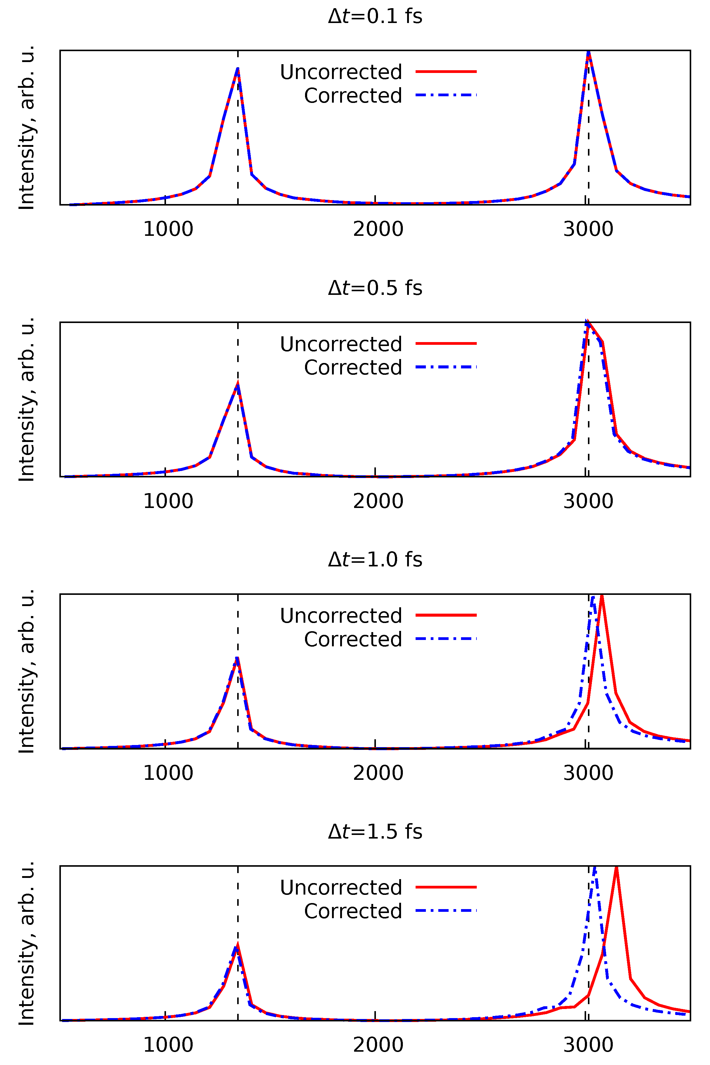
To illustrate this artificial blue shift of vibrational bands and the effectiveness of the correction in Equation 8, we ran four sets of ten N V E -MD trajectories of methane ( CH 4 ) at GFN2-xTB level of theory with initial conditions sampled from the Maxwell-Boltzmann distribution at 300 K, each trajectory was 0.5 ps in length. The sets were differing by the time step Δ t , namely with Δ t = 0.1 , 0.5 , 1.0 , 1.5 fs. The mean vibrational spectra for each set of trajectories and their frequency-corrected counterparts are shown in Figure 2. As one can see, the larger time steps lead to a noticeable shift of the C–H stretching band. In the reference spectrum with Δ t = 0.1 fs such peak is located at approximately 3015 cm−1, whilst at simulations with Δ t = 1.5 fs this peak appears at approximately 3150 cm−1. However, rescaling the frequency axis using Equation 8 restores the positions of the vibrational bands to their correct origin.

3.3. Simplified Wigner Sampling for Generating Initial Conditions

To include the NQEs in the MD simulations, we can use the approach of simplified Wigner sampling (SWS) introduced in Ref. [14]. The sampling relies on generating simultaneously a displacement along the coordinate and momentum axis in a given direction. The displacements are generated using a Gaussian distribution with standard deviations[14]
σ x 2 = τ SWS 2 m
for coordinate and
σ T 2 = m k B T eff
for momentum. Here, = 1.05 × 10 34 J · s is the Planck constant, m is the mass of the nucleus, k B = 1.38 × 10 23 J/K is the Boltzmann constant, τ SWS is a free parameter with the dimension of time, and T eff is the effective temperature defined as
T eff ( T , τ SWS ) = T + 2 k B τ SWS ,
where T 0 is the temperature of the system.
The main problem of the SWS is the choice of the free parameter τ SWS . In work [14], it was proposed to perform several MD simulations with different values of τ SWS and then take the parameter value that minimizes the total energy or the mean temperature of the simulation. In some sense, this approach relates to the variational principle, adjusting the underlying Wigner distribution to fit the PES as well as possible. However, such an approach is quite slow and inefficient. Thus, a cheaper criterion for the choice of τ SWS is required.
To provide an alternative criterion, we may use the harmonic approximation as the guiding principle, as single harmonic frequency calculation with analytical Hessian generally takes less computational time than running multiple MD trajectories. The total kinetic energy of the system is defined as [18]
KE = k = 1 N at p k 2 2 m k ,
where p k is the momentum vector of k-th atom, m k is the mass of the k-th atom, and N at is the total number of atoms in the system. In the case of the distribution sampled at T = 0 with SWS, the mean value of p k 2 is given as p k 2 = 3 σ 0 2 = 3 m k / ( 2 τ ) (see Equation 10). This gives the total mean kinetic energy of KE = 3 N at m k / ( 4 τ ) , while for a given degree of freedom, the mean kinetic energy is KE 1 = KE / ( 3 N at ) = / ( 4 τ ) . In the harmonic approximation, for a given l-th mode ( l = 1 , 2 , , N f , where N f is the number of vibrational degrees of freedom) with vibrational frequency ν l , the kinetic energy is KE l = h ν l / 4 [53], and the mean kinetic energy over all of vibrational modes is
KE h = l = 1 N f h ν l 4 = N f h ν 4 ,
where ν = ( l = 1 N f ν l ) / N f is the mean vibrational frequency of the system. By taking KE 1 = KE h / N f , we arrive at the following expression
τ SWS , h = 1 2 π ν = 2 π 1 N f l = 1 N f ν l ν 1 .
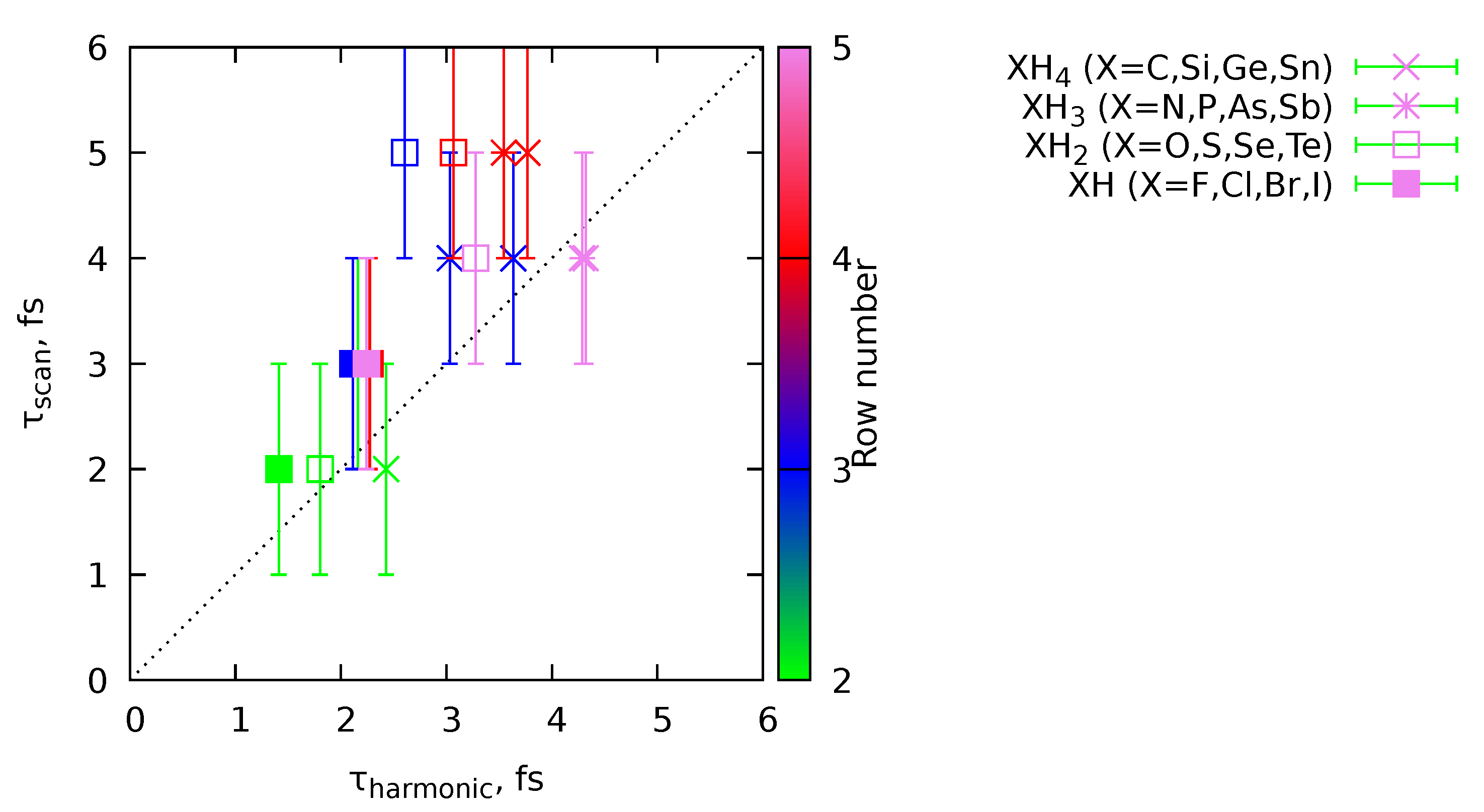
Equation 14 provides a criterion for the choice of τ from the harmonic vibrational frequencies of the system. To show its applicability, we ran a set of N V E -MD calculations for molecules XH ( X = F , Cl , Br , I ), XH2 ( X = O , S , Se , Te ), XH3 ( X = N , P , As , Sb ), and XH4 ( X = C , Si , Ge , Sn ) at the GFN2-xTB level of theory. The MD trajectories were obtained with 1 fs time step for 0.5 ps in total. The τ SWS for SWS initial conditions was scanned from 1 to 10 fs with 1 fs step, and the MD simulation for a given τ SWS contained ten individual trajectories. The optimal τ SWS was chosen as the one minimizing the mean total temperature of the MD simulation. The results are given in Figure 3. As one can see, both criteria correlate with each other (Pearson correlation coefficient is 0.71). Therefore, we can apply the Equation Figure 3 for other molecular systems.

3.4. Thermostats Incorporating Simplified Wigner Sampling

SWS approach, despite being quite crude, has its merits. Unlike the standard Wigner sampling, which can be used only at the beginning of the MD simulation, as the displacements are connected to the equilibrium reference structure, the SWS allows a re-sampling of the displacements during the simulation. This property makes the SWS compatible with canonical ensemble simulations, particularly with Andersen [54] and Berendsen [55] thermostats. Here, we will describe how to do it for both of these thermostats.
The canonical Andersen thermostat works by reassigning the velocity (or of one of the three components) of a randomly chosen atom according to the Maxwell-Boltzmann distributions at random points of MD simulation. The probability of reassignment is given as p A = Δ t / τ A , where τ A is the time of the reassignment. At each point of time, a random number 0 p trial < 1 is generated from the uniform distribution, and if condition p trial < p A is fulfilled, then the velocity reassignment procedure is initiated. Typically, τ A should be greater than the characteristic periods of motions in the system, so the Andersen thermostat does not significantly disrupt the dynamics of the molecule. To combine the Andersen thermostat with the SWS, one has to replace the Maxwell-Boltzmann distribution resampling stage with the SWS routine, sampling both the momentum along given degrees of freedom and the displacement of the coordinate.
The Berendsen thermostat relies on the soft resampling of the velocities at each step of the MD simulation by multiplying them with a scale factor [18,55]
s = 1 + Δ t τ B · T d T ( t ) 1 ,
where τ B is the relaxation time, a free parameter of the Berendsen thermostat, T d is the desired temperature of the MD simulation and T ( t ) is the instant temperature of the nuclei in the MD simulations, defined as T ( t ) = 2 · KE ( t ) / N f with KE being the total kinetic energy of the molecule at time t, and N f is the number of degrees of freedom (i.e., N f = 3 × N at N constr , where N at is the number of atoms in the system and N constr is number of constraints). By replacing the T d with the effective desired temperature according to Equation 11, we also make the Berendsen thermostat compatible with the SWS sampling.

3.5. Scaling of the vibrational spectra from the molecular dynamics

Scaling the harmonic vibrational frequencies and zero-point vibrational energies is a simple yet powerful tool for increasing the accuracy of IR spectra and thermodynamic properties calculations [56]. In the case of vibrational frequencies, the multiplication by a precomputed scale factor for a given method accounts for the systematic errors due to the quantum-chemical approximation quality and the absence of the anharmonic effects [56,57]. Therefore, it seems like a reasonable suggestion to also allow for scaling of the anharmonic spectra from the MD simulations.
Here, we propose the procedure for obtaining the scale factors ( γ ) for IR spectra from the MD and also provide a set of precomputed values for three quantum-chemical approximations: BLYP-D3(BJ)/6-31G, PBE-D3(BJ)/6-31G, and PBEh-3c. For this, we have taken six molecules: water ( H 2 O ), ammonia ( NH 3 ), methane ( CH 4 ), ethane ( C 2 H 6 ), methylamine ( CH 3 NH 2 ), and methanol ( CH 3 OH ). For each of these molecules at each of the quantum-chemical methods, three trajectories were computed using the combination of Andersen and Berendsen thermostats with τ A = 100 fs and τ B = 50 fs and the SWS sampling with the τ SWS taken according to criterion from Equation 14. Each trajectory was at T = 0 K with the time step of Δ t = 1 fs and the total duration of 1 ps. The spectra were computed using the FFT procedure without ignoring the equilibration phase and with the application of the frequency correction from Equation 8. The experimental gas-phase IR spectra of the same molecular species were taken from the NIST Chemistry WebBook [58].
It is not straightforward to compare theoretical spectra with a given frequency increment with their experimental counterparts since they have different frequency increments. Moreover, when the frequency axis is scaled for the spectra from the MD, the frequency increment will also change. Therefore, the following procedure was applied to determine the scale factor of the MD spectra for a given molecule. Let us assume that the MD spectrum is given as a set of M points { ( ν 1 ( MD ) , I 1 ( MD ) ) , ( ν 2 ( MD ) , I 2 ( MD ) ) , ( ν M ( MD ) , I M ( MD ) ) } and the experimental spectrum is a set of N points { ( ν 1 ( exp ) , I 1 ( exp ) ) , ( ν 2 ( exp ) , I 2 ( exp ) ) , ( ν N ( exp ) , I N ( exp ) ) } , where ν i ( X ) and I i ( X ) are the i-th frequency and intensity obtained with method “X”. To remove the rotational substructure of the bands for small molecules, such as water or methane, the experimental data were also smoothed by a convolution with the Gaussian function. The frequency scale factor γ is obtained by maximizing the following expression
C ( γ ) = ( I ( MD ) ) D ( γ ) I ( exp ) max ,
where I ( MD ) and I ( exp ) are the vectors composed of intensity values of N and M dimensions each, and the D ( γ ) is the M × N matrix composed of elements
D i j ( γ ) = exp γ · ν i ( MD ) ν j ( exp ) 2 2 σ 2
with 1 i M , 1 j N , and σ = min ( γ · Δ ν ( MD ) , Δ ν ( exp ) ) with Δ ν being the frequency increments in the respective datasets. The scale factor γ was searched for in the interval 0.8 γ 1.2 .
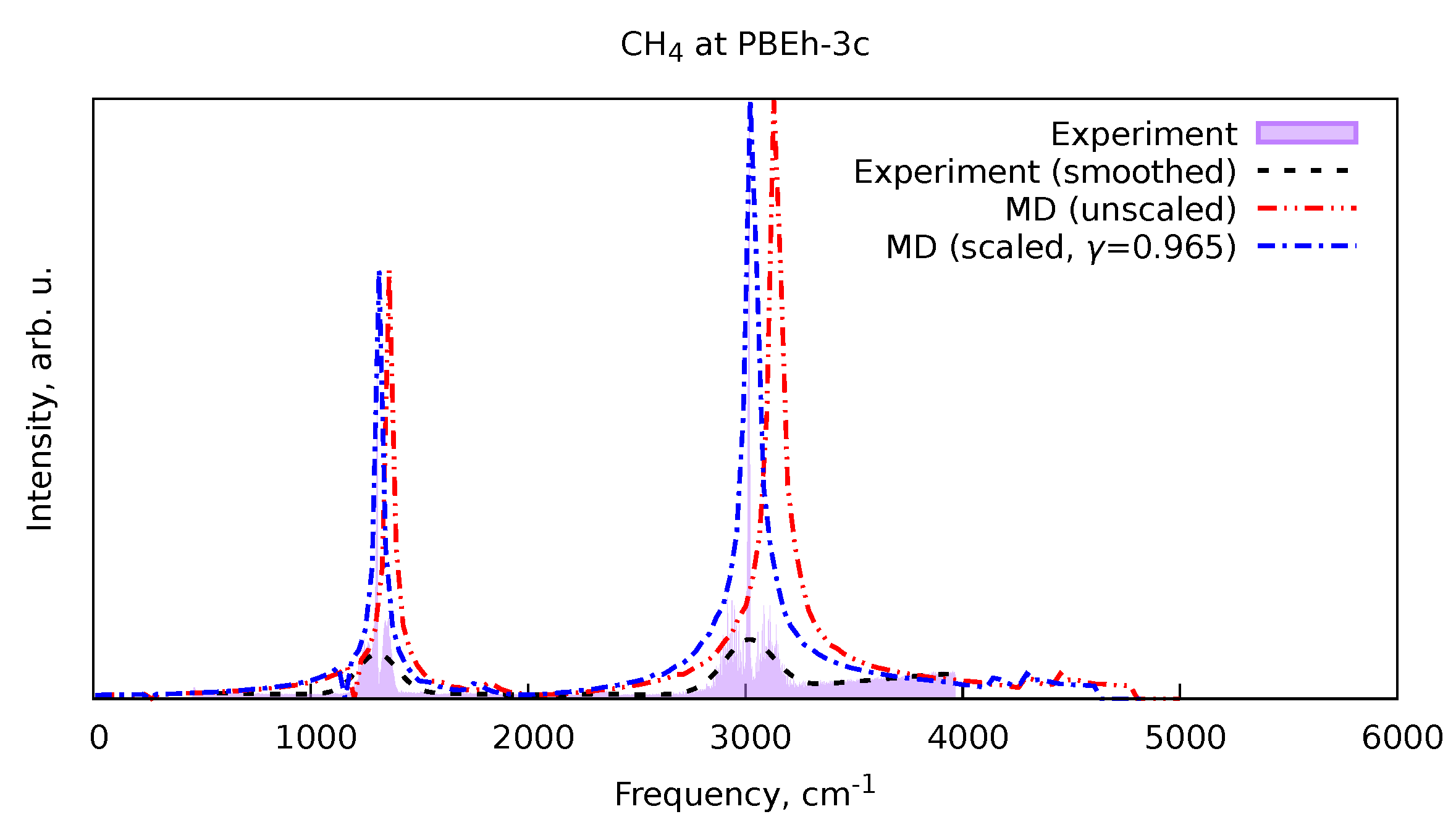
Figure 4 shows an example of the result of the procedure described above. In this Figure, the unscaled and scaled spectra of methane obtained from MD simulations at the PBEh-3c level of theory are shown, as well as the corresponding raw and smoothed experimental data from the NIST Chemistry Webbook. As one can see, the scaling indeed improves the positions of the vibrational bands in the spectra. The scale factors obtained from all the training set molecules were averaged to produce the estimated scale factor for a given level of theory. The results are given in Table 1. In the cases of the BLYP and PBE-based spectra, the ammonia had to be removed from the dataset as the most intense low-frequency vibrational band, corresponding to the valence band vibrations, was too far off from the experimental position.

4. Discussion

In the previous section (Section 3), the protocol for the IR spectra simulations from the AIMD using the PyRAMD was introduced. In an orderly fashion, it looks as follows.
  • First, we need to optimize the structure of the molecule at the given level of theory and compute harmonic vibrational frequencies. Then, using Equation 14, we can calculate the τ SWS parameter to define the SWS sampling routine.
  • Then, we can set the Berendsen and Andersen thermostats for simultaneous usage in the N V T -MD simulation. The combination of the two acts as a friction and random force in more sophisticated thermostats, such as the Langevin-based models [59] (including the color-noise generalized Langevin equation [60]) and the Bussi-Donadio-Parrinello thermostat [61]. This requires setting the two free parameters: relaxation time τ B for the Berendsen thermostat and the resampling time τ A for the Andersen thermostat. The SWS compatibility is assured by using the effective temperature (Equation 11) for the Berendsen thermostat. In the case of the Andersen thermostat, the Maxwell-Bolztmann resampling is replaced with the SWS procedure.
  • Then, a single or a few MD trajectories are collected with reasonably large time steps. The choice criterion is dictated by the integration method and corresponding frequency correction (Equation 8, see also Appendix A). In the cases of Verlet, velocity Verlet, and leapfrog integration schemes, the limit is given as Δ t ( π ν max ) 1 , where ν max is the maximal vibrational frequency of the system. If we take the H-F stretching frequency in hydrofluoric acid ( ν HF = 4138 cm−1[62]), we get the maximal allowed time step of Δ t = 2.6 fs. Therefore, the time steps of around 1 fs are possible for most chemical systems. The total dipole moment of the molecular system is stored at every time step of the MD simulation.
  • After the collection of the trajectory, the vibrational spectrum is computed as the FT of the dipole moment (Equation 2) or its velocity (Equation 3) autocorrelation function (Equation 1). The initial part of the trajectory is usually disregarded as the equilibration phase. The frequency resolution of the FT is given as Δ ν = 1 / τ tot , where τ tot is the total duration of the trajectory (without the equilibration phase). An alternative way to transfer the autocorrelation function from the time domain into the frequency domain with arbitrary frequency increment is the rLSSA routine (Equation 6), albeit this procedure is much more computationally expensive than FFT, thus it makes sense to use it only for short ( 10 3 steps) trajectories.
  • Finally, the frequency correction (Equation 8) is applied, by transforming the frequency axis. Afterward, a tabulated scale factor for the corrected spectrum can be applied to account for the systematic errors in the quantum-chemical approximation.
To illustrate this procedure in action, we will consider a case of protonated methane ( CH 5 + ), with the vibrational spectrum obtained in Ref. [63]. For that, three N V T -MD trajectories at PBEh-3c level of theory with Andersen ( τ A = 150 fs) and Berendsen ( τ B = 50 fs) thermostats were computed. Each trajectory was 3 ps in length with 1 fs time step, and the τ SWS = 4.2 fs was taken from the harmonic frequencies at the same level of theory. After the MD simulations ended, for each of the trajectories, an rLSSA-computed spectrum was obtained with the first 1 ps of each trajectory disregarded for the equilibration phase. The spectra were smoothed by a convolution with Gaussian function with full width at half maximum (FWHM) of 50 cm−1. For this, before performing the rLSSA procedure, the dipole velocity autocorrelation function was multiplied by a Fourier image of the frequency smoothing Gaussian, i.e., with another Gaussian distribution in the time domain with FWHM inversely proportional to the one in the frequency domain. Finally, the frequency correction and scale factor were applied. However, in addition to that, the total intensity in the spectrum was corrected by multiplying with the function of the form[14]
f ( ν ) = 0 , if ν < D , 1 D ν , if ν D ,
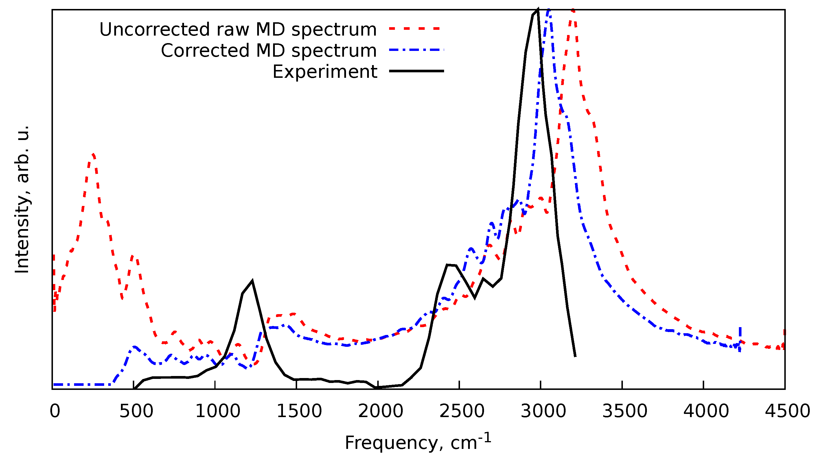
where ν is the frequency in cm−1 and D = 383 cm−1 is the reaction energy needed for the signal to be detected. This type of correction was introduced in Ref. [14] and is not specific to the MD spectra but to the action spectroscopic methods in general. As we can see from Figure 5, the MD routine already produces a decent-looking spectrum. However, the application of the frequency correction, scale factor, and intensity correction (Equation 18) brings the theoretical spectrum quite close to the experimental one.

5. Conclusions

We have presented a general approach for computing the IR spectra of polyatomic systems using the AIMD approach implemented in the PyRAMD software. The approach invokes the following essential components: 1) inclusion of the NQEs by the usage of the SWS approach coupled to the thermostats; 2) frequency correction, allowing for larger time steps in the MD simulations; 3) pre-parametrized scaling factors, similar to those used for the harmonic frequency calculations. The synergistic effect of these components was demonstrated using the test case of the protonated methane. Despite this scheme being inferior to the more direct approaches, such as a combination of path integral MD for inclusion of the NQEs and of the smaller time steps in combination with highly accurate methods to obtain the PES, it was demonstrated that it could produce reasonable results on a fraction of computational time. Therefore, the presented algorithm can be recommended to provide theoretical counterparts to the experimental measurements.

Author Contributions

Conceptualization, D.S.T.; methodology, D.S.T.; validation, D.S.T.; formal analysis, D.S.T.; investigation, D.S.T.; writing—original draft preparation, D.S.T.; visualization, D.S.T.; All authors have read and agreed to the published version of the manuscript.

Data Availability Statement

All software, simulation scripts, and the results are available in the Zenodo repository at DOI: 10.5281/zenodo.12744805.

Acknowledgments

This work has been supported by Deutsches Elektronen-Synchtrotron DESY, a member of the Helmholtz Association (HGF). Calculations were enabled through the Maxwell computational resources operated at Deutsches Elektronen-Synchrotron DESY, Hamburg, Germany.

Abbreviations

The following abbreviations are used in this manuscript:
AIMD ab initio molecular dynamics
FFT fast Fourier transform
FT Fourier transform
IR infrared
MD molecular dynamics
NQE nuclear quantum effect
NSK Nyquist–Shannon–Kotelnikov (theorem)
PES potential energy surface
rLSSA regularized least-squares spectral analysis
rwLSSA regularized weighted least-squares spectral analysis
SWS simplified Wigner sampling

Appendix A. Derivation of high-order frequency correction

Let us consider the numerical evolution of the one-dimensional harmonic oscillator with Hooke’s force given as F = m ω 2 x with m being the oscillator mass, ω – the real vibrational angular frequency related to the normal one as ω = 2 π ν and x is the position of the oscillator [40]. By using the Taylor expansion of the coordinate in time near time t, we get
x ( t ± Δ t ) = x ( t ) ± x ˙ ( t ) Δ t + 1 2 x ¨ ( t ) Δ t 2 ± 1 6 x ( t ) Δ t 3 + 1 24 x ( t ) Δ t 4 ,
where the number of dots above x denotes the time derivative order. Thus, by summing these symmetrical displacements, we get rid of odd-power Δ t n terms and arrive at
x ( t + Δ t ) + x ( t Δ t ) = 2 x ( t ) + x ¨ ( t ) Δ t 2 + 1 12 x ( t ) Δ t 4 .
If we ignore the fourth-order time derivative x ( t ) , we arrive at the Verlet integration algorithm. To find the viable expression for x ( t ) , let us also do a Taylor expansion of the acceleration x ¨ near time t, as
x ¨ ( t ± Δ t ) = x ¨ ( t ) ± x ( t ) Δ t + 1 2 x ( t ) Δ t 2 ,
from where (similarly to Equation A1) we arrive at
x ¨ ( t + Δ t ) + x ¨ ( t Δ t ) = 2 x ¨ ( t ) + x ( t ) Δ t 2 ,
and thus
x ( t ) Δ t 2 = x ¨ ( t + Δ t ) 2 x ¨ ( t ) + x ¨ ( t Δ t ) .
Substituting this approximation for x ( t ) Δ t 2 into the Equation A1, we get
x ( t + Δ t ) + x ( t Δ t ) = 2 x ( t ) + x ¨ ( t ) Δ t 2 + 1 12 x ¨ ( t + Δ t ) 2 x ¨ ( t ) + x ¨ ( t Δ t ) Δ t 2 .
To evaluate the time behavior of the harmonic oscillator, we assume that the numerically integrated behavior is x ( t ) = A cos ( ω ˜ t ) [40], where A is the amplitude of the motion, ω ˜ is the effective frequency, and the phase of initial conditions is chosen to be zero. In this case, the acceleration, according to the second Newton’s law, is F = m x ¨ ( t ) = m ω 2 x ( t ) , thus x ¨ ( t ) = ω 2 x ( t ) . Substituting all of that into the Equation A2, we get
A · cos ( ω ˜ t + ω ˜ Δ t ) + cos ( ω ˜ t ω ˜ Δ t ) = = 2 A cos ( ω ˜ t ) ω 2 Δ t 2 A cos ( ω ˜ t ) A ω 2 Δ t 2 12 cos ( ω ˜ t + ω ˜ Δ t ) 2 cos ( ω ˜ t ) + cos ( ω ˜ t ω ˜ Δ t ) .
As cos ( ω ˜ t ± ω ˜ Δ t ) = cos ( ω ˜ t ) cos ( ω ˜ Δ t ) sin ( ω ˜ t ) sin ( ω ˜ Δ t ) , we get that
cos ( ω ˜ t + ω ˜ Δ t ) + cos ( ω ˜ t ω ˜ Δ t ) = 2 cos ( ω ˜ t ) cos ( ω ˜ Δ t ) .
Substituting this equation into the Equation A3, and dividing it by 2 x ( t ) = 2 A cos ( ω ˜ t ) , we get
cos ( ω ˜ Δ t ) = 1 ω 2 Δ t 2 2 ω 2 Δ t 2 12 cos ( ω ˜ Δ t ) 1 ,
which, upon considering 1 cos ( ω ˜ Δ t ) = 2 sin 2 ω ˜ Δ t / 2 , we can rearrange as
ω 2 Δ t 2 2 · 1 1 3 sin 2 ω ˜ Δ t 2 = 2 sin 2 ω ˜ Δ t 2 .
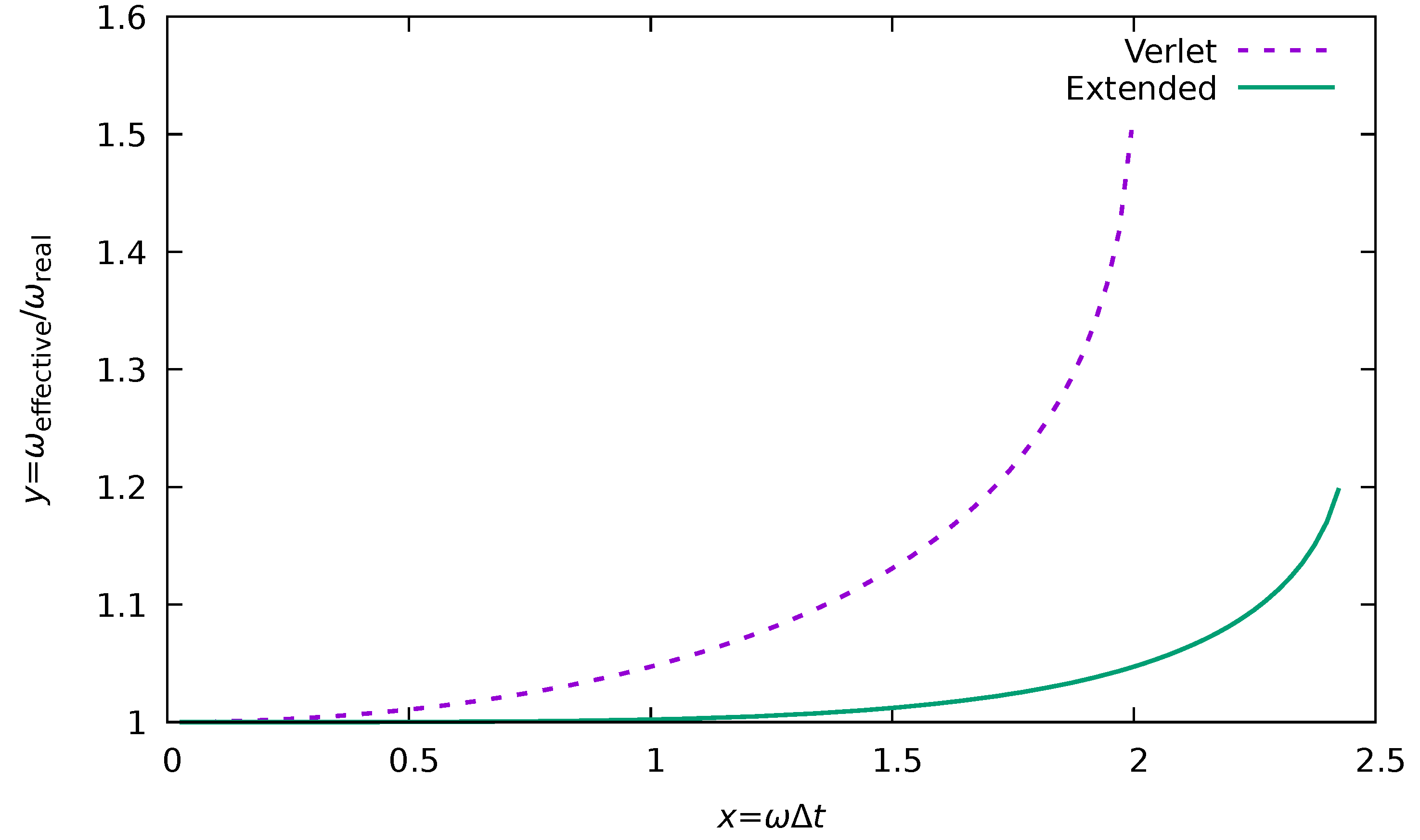
This expression provides a correction of the observed frequency ω ˜ to the real one, as ω = ω ( ω ˜ ) . If the term sin 2 ( ω ˜ Δ t / 2 ) / 3 in the left side of the Equation A4 will be ignored, it will correspond to the Verlet integration, and after rearrangement, we arrive at the Equation 8.
To illustrate the actual shift of the real frequency ω into the effective one ( ω ˜ ), we can rearrange the Equation A4 as
ω ˜ Δ t = 2 arcsin ω Δ t 2 1 + ω 2 Δ t 2 12 .
We can introduce a new variable x = ω Δ t , which shows how many parts of the true vibrational period τ = 2 π / ω the time step Δ t spans as Δ t = x / ω = τ · x / ( 2 π ) . In this case, we can track the relative shift of the vibrational frequency y = ω ˜ / ω as
y = ω ˜ ω = 2 x · arcsin x 2 1 + x 2 12 .
In the case of the Verlet algorithm, the equation is the same, but 1 + x 2 12 needs to be replaced by 1, i.e.,
y Verlet = ω ˜ ω = 2 x · arcsin x 2 .
The comparison of these frequency shifts can be found in Figure A1. As one can see, the higher-order integration schemes produce significantly smaller frequency shifts compared to the Verlet integration algorithm. Secondly, they should allow for larger limiting frequencies. The applicability limits of the Equations A5 and A6 are given by the domain of the arcsine function. Therefore, in the case of Verlet correction (Equation A6), it is given as x / 2 1 , i.e., x = ω Δ t 2 . For the higher order correction (Equation A5), the limit is given by
x 2 1 + x 2 12 1 ,
which is equivalent to x = ω Δ t 6 2.4 .
Figure A1. Comparison of the relative frequency shifts in the Verlet integration (Equation A6) and the higher order method (Equation A5).
Preprints 112273 g0a1

References

  1. Levitt, M. Birth and Future of Multiscale Modeling for Macromolecular Systems (Nobel Lecture). Angewandte Chemie International Edition 2014, 53, 10006–10018. [Google Scholar] [CrossRef] [PubMed]
  2. Karplus, M. Development of Multiscale Models for Complex Chemical Systems: From H+H2 to Biomolecules (Nobel Lecture). Angewandte Chemie International Edition 2014, 53, 9992–10005. [Google Scholar] [CrossRef] [PubMed]
  3. Hollingsworth, S.A.; Dror, R.O. Molecular Dynamics Simulation for All. Neuron 2018, 99, 1129–1143. [Google Scholar] [CrossRef] [PubMed]
  4. Iftimie, R.; Minary, P.; Tuckerman, M.E. Ab initio molecular dynamics: Concepts, recent developments, and future trends. Proceedings of the National Academy of Sciences 2005, 102, 6654–6659. [Google Scholar] [CrossRef] [PubMed]
  5. Thomas, M.; Brehm, M.; Fligg, R.; Vöhringer, P.; Kirchner, B. Computing vibrational spectra from ab initio molecular dynamics. Phys. Chem. Chem. Phys. 2013, 15, 6608–6622. [Google Scholar] [CrossRef] [PubMed]
  6. Wilhelm, J.; VandeVondele, J.; Rybkin, V.V. Dynamics of the Bulk Hydrated Electron from Many-Body Wave-Function Theory. Angewandte Chemie International Edition 2019, 58, 3890–3893. [Google Scholar] [CrossRef] [PubMed]
  7. Levashov, V.A.; Billinge, S.J.L.; Thorpe, M.F. Quantum correction to the pair distribution function. Journal of Computational Chemistry 2007, 28, 1865–1882. [Google Scholar] [CrossRef] [PubMed]
  8. Vishnevskiy, Y.V.; Tikhonov, D. Quantum corrections to parameters of interatomic distance distributions in molecular dynamics simulations. Theoretical Chemistry Accounts 2016, 135, 88. [Google Scholar] [CrossRef]
  9. Tikhonov, D.S.; Otlyotov, A.A.; Rybkin, V.V. The effect of molecular dynamics sampling on the calculated observable gas-phase structures. Phys. Chem. Chem. Phys. 2016, 18, 18237–18245. [Google Scholar] [CrossRef]
  10. Tikhonov, D.S.; Sharapa, D.I.; Schwabedissen, J.; Rybkin, V.V. Application of classical simulations for the computation of vibrational properties of free molecules. Phys. Chem. Chem. Phys. 2016, 18, 28325–28338. [Google Scholar] [CrossRef]
  11. Lan, J.; Kapil, V.; Gasparotto, P.; Ceriotti, M.; Iannuzzi, M.; Rybkin, V.V. Simulating the ghost: quantum dynamics of the solvated electron. Nature Communications 2021, 12, 766. [Google Scholar] [CrossRef]
  12. Höfener, S.; Trumm, M.; Koke, C.; Heuser, J.; Ekström, U.; Skerencak-Frech, A.; Schimmelpfennig, B.; Panak, P.J. Computing UV/vis spectra using a combined molecular dynamics and quantum chemistry approach: bis-triazin-pyridine (BTP) ligands studied in solution. Phys. Chem. Chem. Phys. 2016, 18, 7728–7736. [Google Scholar] [CrossRef]
  13. Ditler, E.; Luber, S. Vibrational spectroscopy by means of first-principles molecular dynamics simulations. WIREs Computational Molecular Science 2022, 12, e1605. [Google Scholar] [CrossRef]
  14. Tikhonov, D.S.; Vishnevskiy, Y.V. Describing nuclear quantum effects in vibrational properties using molecular dynamics with Wigner sampling. Phys. Chem. Chem. Phys. 2023, 25, 18406–18423. [Google Scholar] [CrossRef] [PubMed]
  15. Scherrer, A.; Vuilleumier, R.; Sebastiani, D. Vibrational circular dichroism from ab initio molecular dynamics and nuclear velocity perturbation theory in the liquid phase. The Journal of Chemical Physics 2016, 145, 084101. [Google Scholar] [CrossRef]
  16. Kubo, R. The fluctuation-dissipation theorem. Reports on Progress in Physics 1966, 29, 255. [Google Scholar] [CrossRef]
  17. Landau, L.; Lifshitz, E. Statistical Physics: Volume 5; Number Bd. 5, Elsevier Science, 2013. [Google Scholar]
  18. Schlick, T. Molecular Dynamics: Basics. In Molecular Modeling and Simulation: An Interdisciplinary Guide: An Interdisciplinary Guide; Springer New York: New York, NY, 2010; pp. 425–461. [Google Scholar] [CrossRef]
  19. Markland, T.E.; Ceriotti, M. Nuclear quantum effects enter the mainstream. Nature Reviews Chemistry 2018, 2, 0109. [Google Scholar] [CrossRef]
  20. Marx, D.; Parrinello, M. Ab initio path integral molecular dynamics: Basic ideas. The Journal of Chemical Physics 1996, 104, 4077–4082. [Google Scholar] [CrossRef]
  21. Althorpe, S.C. Path-integral approximations to quantum dynamics. The European Physical Journal B 2021, 94, 155. [Google Scholar] [CrossRef]
  22. Ceriotti, M.; Bussi, G.; Parrinello, M. Nuclear Quantum Effects in Solids Using a Colored-Noise Thermostat. Phys. Rev. Lett. 2009, 103, 030603. [Google Scholar] [CrossRef]
  23. Zobel, J.P.; Nogueira, J.J.; González, L. Finite-temperature Wigner phase-space sampling and temperature effects on the excited-state dynamics of 2-nitronaphthalene. Phys. Chem. Chem. Phys. 2019, 21, 13906–13915. [Google Scholar] [CrossRef] [PubMed]
  24. Zobel, J.P.; Heindl, M.; Nogueira, J.J.; González, L. Vibrational Sampling and Solvent Effects on the Electronic Structure of the Absorption Spectrum of 2-Nitronaphthalene. Journal of Chemical Theory and Computation 2018, 14, 3205–3217. [Google Scholar] [CrossRef] [PubMed]
  25. Neese, F. Software update: The ORCA program system—Version 5.0. WIREs Computational Molecular Science 2022, 12, e1606. [Google Scholar] [CrossRef]
  26. Bannwarth, C.; Caldeweyher, E.; Ehlert, S.; Hansen, A.; Pracht, P.; Seibert, J.; Spicher, S.; Grimme, S. Extended tight-binding quantum chemistry methods. WIREs Computational Molecular Science 2021, 11, e1493. [Google Scholar] [CrossRef]
  27. Tikhonov, D.S. Metadynamics simulations with Bohmian-style bias potential. Journal of Computational Chemistry 2023, 44, 1771–1775. [Google Scholar] [CrossRef] [PubMed]
  28. Tikhonov, D.S.; Datta, A.; Chopra, P.; Steber, A.L.; Manschwetus, B.; Schnell, M. Approaching black-box calculations of pump-probe fragmentation dynamics of polyatomic molecules. Zeitschrift für Physikalische Chemie 2020, 234, 1507–1531. [Google Scholar] [CrossRef]
  29. Tikhonov, D.S. PyRAMD. 2024. Available online: https://gitlab.desy.de/denis.tikhonov/pyramd.
  30. Kohn, W. Nobel Lecture: Electronic structure of matter—wave functions and density functionals. Rev. Mod. Phys. 1999, 71, 1253–1266. [Google Scholar] [CrossRef]
  31. Becke, A.D. Density-functional exchange-energy approximation with correct asymptotic behavior. Phys. Rev. A 1988, 38, 3098–3100. [Google Scholar] [CrossRef] [PubMed]
  32. Lee, C.; Yang, W.; Parr, R.G. Development of the Colle-Salvetti correlation-energy formula into a functional of the electron density. Phys. Rev. B 1988, 37, 785–789. [Google Scholar] [CrossRef]
  33. Grimme, S.; Ehrlich, S.; Goerigk, L. Effect of the damping function in dispersion corrected density functional theory. Journal of Computational Chemistry 2011, 32, 1456–1465. [Google Scholar] [CrossRef]
  34. Hehre, W.J.; Ditchfield, R.; Pople, J.A. Self—Consistent Molecular Orbital Methods. XII. Further Extensions of Gaussian—Type Basis Sets for Use in Molecular Orbital Studies of Organic Molecules. The Journal of Chemical Physics 1972, 56, 2257–2261. [Google Scholar] [CrossRef]
  35. Perdew, J.P.; Burke, K.; Ernzerhof, M. Generalized Gradient Approximation Made Simple [Phys. Rev. Lett. 77, 3865 (1996)]. Phys. Rev. Lett. 1997, 78, 1396–1396. [Google Scholar] [CrossRef]
  36. Grimme, S.; Brandenburg, J.G.; Bannwarth, C.; Hansen, A. Consistent structures and interactions by density functional theory with small atomic orbital basis sets. The Journal of Chemical Physics 2015, 143, 054107. [Google Scholar] [CrossRef] [PubMed]
  37. Bannwarth, C.; Ehlert, S.; Grimme, S. GFN2-xTB—An Accurate and Broadly Parametrized Self-Consistent Tight-Binding Quantum Chemical Method with Multipole Electrostatics and Density-Dependent Dispersion Contributions. Journal of Chemical Theory and Computation 2019, 15, 1652–1671. [Google Scholar] [CrossRef] [PubMed]
  38. Press, W.H.; Teukolsky, S.A.; Vetterling, W.T.; Flannery, B.P. Numerical Recipes 3rd Edition: The Art of Scientific Computing, 3 ed.; Cambridge University Press: USA, 2007. [Google Scholar]
  39. Tikhonov, D.S. Regularized weighted sine least-squares spectral analysis for gas electron diffraction data. The Journal of Chemical Physics 2023, 159, 174101. [Google Scholar] [CrossRef] [PubMed]
  40. Tikhonov, D.S. Simple posterior frequency correction for vibrational spectra from molecular dynamics. The Journal of Chemical Physics 2016, 144, 174108. [Google Scholar] [CrossRef] [PubMed]
  41. Harris, C.R.; Millman, K.J.; van der Walt, S.J.; Gommers, R.; Virtanen, P.; Cournapeau, D.; Wieser, E.; Taylor, J.; Berg, S.; Smith, N.J.; Kern, R.; Picus, M.; Hoyer, S.; van Kerkwijk, M.H.; Brett, M.; Haldane, A.; del Río, J.F.; Wiebe, M.; Peterson, P.; Gérard-Marchant, P.; Sheppard, K.; Reddy, T.; Weckesser, W.; Abbasi, H.; Gohlke, C.; Oliphant, T.E. Array programming with NumPy. Nature 2020, 585, 357–362. [Google Scholar] [CrossRef] [PubMed]
  42. Virtanen, P.; Gommers, R.; Oliphant, T.E.; Haberland, M.; Reddy, T.; Cournapeau, D.; Burovski, E.; Peterson, P.; Weckesser, W.; Bright, J.; van der Walt, S.J.; Brett, M.; Wilson, J.; Millman, K.J.; Mayorov, N.; Nelson, A.R.J.; Jones, E.; Kern, R.; Larson, E.; Carey, C.J.; Polat, İ.; Feng, Y.; Moore, E.W.; VanderPlas, J.; Laxalde, D.; Perktold, J.; Cimrman, R.; Henriksen, I.; Quintero, E.A.; Harris, C.R.; Archibald, A.M.; Ribeiro, A.H.; Pedregosa, F.; van Mulbregt, P. SciPy 1.0 Contributors. SciPy 1.0: Fundamental Algorithms for Scientific Computing in Python. Nature Methods 2020, 17, 261–272. [Google Scholar] [CrossRef]
  43. Ivanov, S.D.; Witt, A.; Marx, D. Theoretical spectroscopy using molecular dynamics: theory and application to CH5+ and its isotopologues. Phys. Chem. Chem. Phys. 2013, 15, 10270–10299. [Google Scholar] [CrossRef]
  44. Cooley, J.; Tukey, J. An Algorithm for the Machine Calculation of Complex Fourier Series. Mathematics of Computation 1965, 19, 297–301. [Google Scholar] [CrossRef]
  45. Shannon, C. Communication in the Presence of Noise. Proceedings of the IRE 1949, 37, 10–21. [Google Scholar] [CrossRef]
  46. Nyquist, H. Certain Topics in Telegraph Transmission Theory. Transactions of the American Institute of Electrical Engineers 1928, 47, 617–644. [Google Scholar] [CrossRef]
  47. Kotel’nikov, V.A. On the transmission capacity of ’ether’ and wire in electric communications. Phys. Usp. 2006, 49, 736–744. [Google Scholar] [CrossRef]
  48. Brehm, M.; Thomas, M.; Gehrke, S.; Kirchner, B. TRAVIS—A free analyzer for trajectories from molecular simulation. The Journal of Chemical Physics 2020, 152, 164105. [Google Scholar] [CrossRef] [PubMed]
  49. Tikhonov, D.S.; Garg, D.; Schnell, M. Inverse Problems in Pump–Probe Spectroscopy. Photochem 2024, 4, 57–110. [Google Scholar] [CrossRef]
  50. Praprotnik, M.; Janežič, D. Molecular dynamics integration and molecular vibrational theory. III. The infrared spectrum of water. The Journal of Chemical Physics 2005, 122, 174103. [Google Scholar] [CrossRef]
  51. Horníček, J.; Kaprálová, P.; Bouř, P. Simulations of vibrational spectra from classical trajectories: Calibration with ab initio force fields. The Journal of Chemical Physics 2007, 127, 084502. [Google Scholar] [CrossRef] [PubMed]
  52. Thomas, M. Methodological Developments. In Theoretical Modeling of Vibrational Spectra in the Liquid Phase; Springer International Publishing: Cham, 2017; pp. 33–83. [Google Scholar] [CrossRef]
  53. Atkins, P.; Paula, J. Atkins’ physical chemistry; Oxford University press, 2008. [Google Scholar]
  54. Andersen, H.C. Molecular dynamics simulations at constant pressure and/or temperature. The Journal of Chemical Physics 1980, 72, 2384–2393. [Google Scholar] [CrossRef]
  55. Berendsen, H.J.C.; Postma, J.P.M.; van Gunsteren, W.F.; DiNola, A.; Haak, J.R. Molecular dynamics with coupling to an external bath. The Journal of Chemical Physics 1984, 81, 3684–3690. [Google Scholar] [CrossRef]
  56. Kesharwani, M.K.; Brauer, B.; Martin, J.M.L. Frequency and Zero-Point Vibrational Energy Scale Factors for Double-Hybrid Density Functionals (and Other Selected Methods): Can Anharmonic Force Fields Be Avoided? The Journal of Physical Chemistry A 2015, 119, 1701–1714. [Google Scholar] [CrossRef] [PubMed]
  57. Tikhonov, D.S.; Gordiy, I.; Iakovlev, D.A.; Gorislav, A.A.; Kalinin, M.A.; Nikolenko, S.A.; Malaskeevich, K.M.; Yureva, K.; Matsokin, N.A.; Schnell, M. Harmonic scale factors of fundamental transitions for dispersion-corrected quantum chemical methods.
  58. Henry M. Rosenstock, Keith Draxl, Bruce W. Steiner, and John T. Herron, "Ion Energetics Data" in NIST Chemistry WebBook, NIST Standard Reference Database Number 69, Eds. P.J. Linstrom and W.G. Mallard, National Institute of Standards and Technology, Gaithersburg MD, 20899, https://doi.org/10.18434/T4D303, (retrieved April 13, 2023).
  59. Schlick, T. Molecular Dynamics: Further Topics. In Molecular Modeling and Simulation: An Interdisciplinary Guide: An Interdisciplinary Guide; Springer New York: New York, NY, 2010; pp. 463–517. [Google Scholar] [CrossRef]
  60. Ceriotti, M.; Bussi, G.; Parrinello, M. Langevin Equation with Colored Noise for Constant-Temperature Molecular Dynamics Simulations. Phys. Rev. Lett. 2009, 102, 020601. [Google Scholar] [CrossRef] [PubMed]
  61. Bussi, G.; Donadio, D.; Parrinello, M. Canonical sampling through velocity rescaling. The Journal of Chemical Physics 2007, 126, 014101. [Google Scholar] [CrossRef] [PubMed]
  62. NIST Computational Chemistry Comparison and Benchmark Database, NIST Standard Reference Database Number 101 Release 22, May 2022, Editor: Russell D. Johnson III URL http://cccbdb.nist.gov/.
  63. Asvany, O.; Kumar, P.; Redlich, B.; Hegemann, I.; Schlemmer, S.; Marx, D. Understanding the Infrared Spectrum of Bare CH5+. Science 2005, 309, 1219–1222. [Google Scholar] [CrossRef] [PubMed]
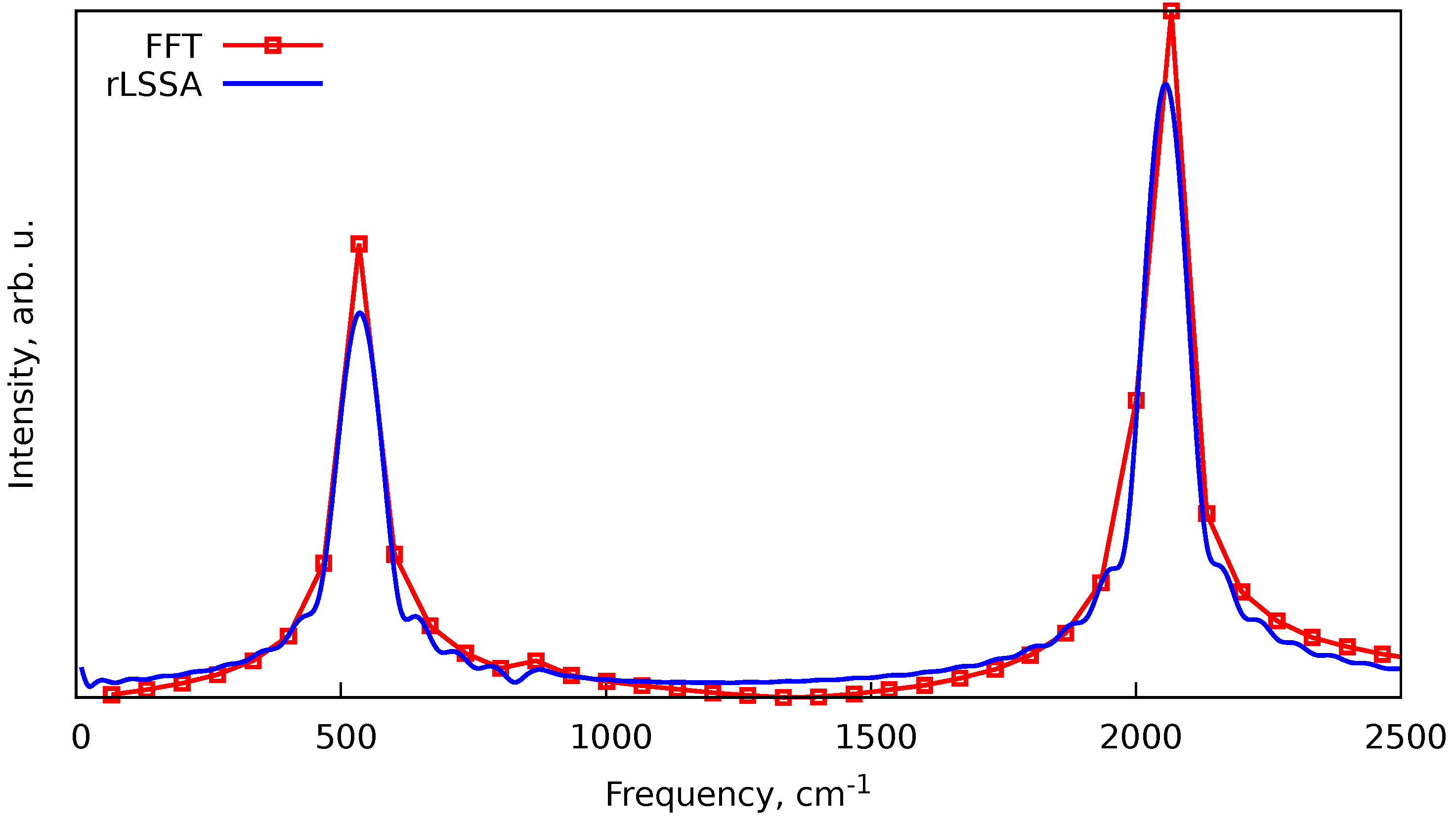
Figure 1. Comparison of the FFT and rLSSA approaches for obtaining spectra from short trajectories. The spectra represent the vibrational spectra of the carbon dioxide obtained from the MD simulations at 300 K with the Berendsen thermostat. The details of MD simulations are given in the text.
Preprints 112273 g001
Figure 2. Effect of the time step ( Δ t ) choice on the vibrational spectra of the methane ( CH 4 ) obtained from the N V E -MD simulations and the action of the frequency correction from the Equation 8. Details of the simulations are given in the text.
Preprints 112273 g002
Figure 3. Comparison of the optimal τ SWS parameters for the SWS sampling obtained from the scan of τ SWS ( τ scan ) and from the Equation 14 ( τ harmonic ).
Preprints 112273 g003
Figure 4. Vibrational spectrum of methane ( CH 4 ), computed at the PBEh-3c level of theory, its scaled version with respect to the smoothed experimental data, according to Equation 16, and the raw and smoothed experimental data from the NIST Chemistry Webbook.
Preprints 112273 g004
Figure 5. Experimental and theoretical IR action spectra of the protonated methane ( CH 5 + ). Theoretical spectra were obtained at the PBEh-3c level of theory. The uncorrected spectrum (red dashed line) corresponds to the direct result of the MD simulations. The corrected spectrum (blue dashed and dotted line) is the same data set but with the frequency correction (Equation 8), scaling factor 0.968 (Table 1), and intensity correction (Equation 18) applied.
Preprints 112273 g005
Table 1. Tabulated scale factors γ for the MD-based vibrational spectra at various levels of theory.
Method Scale factor γ
BLYP-D3(BJ)/6-31G 1.046 ± 0.040
PBE-D3(BJ)/6-31G 1.041 ± 0.046
PBEh-3c 0.968 ± 0.006
Disclaimer/Publisher’s Note: The statements, opinions and data contained in all publications are solely those of the individual author(s) and contributor(s) and not of MDPI and/or the editor(s). MDPI and/or the editor(s) disclaim responsibility for any injury to people or property resulting from any ideas, methods, instructions or products referred to in the content.
Copyright: This open access article is published under a Creative Commons CC BY 4.0 license, which permit the free download, distribution, and reuse, provided that the author and preprint are cited in any reuse.
Prerpints.org logo

Preprints.org is a free preprint server supported by MDPI in Basel, Switzerland.

Subscribe

© 2024 MDPI (Basel, Switzerland) unless otherwise stated